The effect of Poynting-Robertson drag on the triangular Lagrangian points

Abstract

We investigate the stability of motion close to the Lagrangian equilibrium points $L_{4}$ and $L_{5}$ in the framework of the spatial, elliptic, restricted three-body problem, subject to the radial component of Poynting-Robertson drag. For this reason we develop a simplified resonant model, that is based on averaging theory, i.e. averaged over the mean anomaly of the perturbing planet. We find temporary stability of particles displaying a tadpole motion in the 1:1 resonance. From the linear stability study of the averaged simplified resonant model, we find that the time of temporary stability is proportional to $\beta\ a_{1}\ n_{1}$, where $\beta$ is the ratio of the solar radiation over the gravitational force, and $a_{1}$, $n_{1}$ are the semi-major axis and the mean motion of the perturbing planet, respectively. We extend previous results (Murray (1994)) on the asymmetry of the stability indices of $L_{4}$ and $L_{5}$ to a more realistic force model. Our analytical results are supported by means of numerical simulations. We implement our study to Jupiter-like perturbing planets, that are also found in extra-solar planetary systems.

1 Introduction

The motivation of our study is to understand better the effect of stellar radiation on resonant interactions between the motion of dust and a planet in planetary systems. The subject has already been studied in Dermott et al. (1994), where the authors propose that dust may be transported from the main belt to the Earth by temporary resonant capture; the trapping mechanism for exterior mean motion resonances (MMRs) has been studied in full detail in Beaugé and Ferraz-Mello (1994); Weidenschilling and Jackson (1993). Only outer resonances have been found to be stable (see Sicardy et al. (1993) and references therein); the effect of drag on motions close to the Lagrange points is treated in Murray (1994), where the author finds asymmetric stability indices for the triangular points. The three-dimensional orbital evolution of dust particles is also studied in Liou and Zook (1997); Liou et al. (1995). Kortenkamp (2013) has demonstrated a trapping mechanism of dust particles in Earth’s quasi-satellite resonance. The literature on the subject is wide and we refer the reader to the bibliography.

The goals of this paper are the following: i) most analytical studies mentioned above are based on the circular or/and planar, restricted, three-body problem; we therefore aim to extend these results to the case of the spatial, elliptic, restricted three-body problem (SERTBP); this is of particular importance, since stellar radiation forces act in 3D space. ii) The 1:1 MMR under Poynting-Robertson (hereafter PR) effect is only poorly studied by analytical means (with some exception found in Murray (1994) - but based on the circular problem); the reason can maybe found in the fact that standard expansions of the perturbing function do not converge if the ratio of the semi-major axes of the perturber and dust particle tends to unity; we therefore aim to use the equilateral perturbing function instead of the standard one to properly treat the case of the 1:1 MMR. iii) It is commonly accepted that Poynting-Robertson drag destabilizes inner resonances with an external perturber, while temporary capture may be found for outer resonances with an internal perturber (Beaugé and Ferraz-Mello (1994)); we therefore aim to provide with this study the missing link with the co-orbital resonant regime of motion.

There are different kinds of forces that need to be taken into account to model the dynamics of interplanetary dust, that strongly depend on the size of the particles of interest (Gustafson (1994)): solar gravity, stellar radiation pressure, the Lorentz force, planetary perturbations, PR drag, and solar wind drag. In our study we concentrate on particles within the size range from $1\ \mu m$ to $200\ \mu m$, where the Lorentz force can be safely neglected, the primary force is solar gravity and stellar radiation pressure, second order effects are additional planetary perturbations, about the same order of the PR effect. Precisely, we are interested in the interplay of these second order effects on motion of dust particles that are situated inside the 1:1 mean motion resonance with a planet. As we will show the PR effect does not only strongly influence the orbital life-time of particles, but also the location of the resonance in the orbital element space of the interplanetary dust particle.

The models describing the three-body problem are introduced in order of increasing difficulty: from the circular-planar case to the elliptic-inclined one. The models include the effect of Poynting-Robertson drag. Three case studies are identified: Jupiter and two samples, which are representative of extrasolar planetary systems. Using the equations of motion averaged over the mean anomaly, we are able to detect stationary solutions and to describe them in terms of the parameters of the system. We also add a discussion about the eigenvalues of the linearized vector field as a function of the dissipative parameter. We conclude wih a comparison with the unaveraged vector field.

The content of this paper is the following. In Section 2 we define the mathematical model and the equations of motion that we use for our study. In Section 3 we derive a resonant model, valid close to the 1:1 resonance that is based on averaging theory. We investigate the equilibria of the averaged problem in the framework of the planar, spatial, circular and elliptic restricted three body problems in Section 4, and perform a linear stability study of the SERTBP in Section 5. A numerical survey based on the unaveraged equations of motions can be found in Section 6. A summary of our conclusions is given in Section 7; supplementary calculations that may help the reader to reproduce our results can be found in the Appendices.

2 Mathematical model and case studies

We investigate the dynamics of dust-size particles in the framework of the spatial, elliptic restricted three-body problem (SERTBP), in which the central body is the source of electromagnetic radiation, while the second largest body does not radiate. We denote the celestial bodies involved in our model, respectively as the central body (e.g., the star), the secondary body (e.g., a planet), and the third body (e.g., a dust particle). The third body is thus subject to two different kinds of forces, as described below.

• Gravitational Attraction (GA)

  Let $\vec{r}$, $\vec{r}_{1}$ be the vectors of the third and the secondary from the central body in a coordinate system with the origin coinciding with the central body. We denote by $r=\|\vec{r}\|$, $r_{1}=\|\vec{r}_{1}\|$ the distances of the third and the secondary from the origin, and by $\Delta$ the mutual distance of the third and the secondary bodies. Let ${\mathcal{G}}$ be the gravitational constant, and $m_{0}$, $m_{1}$, $m$ be the mass of the central, the secondary, and the third body, respectively. In this setting, the gravitational force can be derived from the force function

  $$U_{grav}=-\frac{{\mathcal{G}}(m_{0}+m)}{r}-{\mathcal{G}}m_{1}\big{(}\frac{1}{\Delta}-\frac{\vec{r}\cdot\vec{r}_{1}}{r_{1}^{3}}\big{)}\ .$$ (1)

  As it is standard in the restricted three body problem, we assume that the third body does not influence the motion of the other two bodies, and formally we set $m=0$.

• Solar Radiation (SR)

  Let $\hat{r}=\vec{r}/r$ be the radial unit vector, $\dot{r}=dr/dt$ be the radial velocity, and $\vec{v}=d{\vec{r}}/dt$ be the instantaneous velocity vector of the third mass. We denote by the dimensionless parameter $\beta$ the ratio of the radiation pressure force that is felt by a particle of radius $r_{p}$ and density $\rho$, over the gravitational force of the central body of mass $m_{0}$ at distance $r$. Let $c$ be the speed of light and $\gamma\equiv 1+s_{w}$, where $s_{w}$ is the ratio of the net force of solar wind over the net force due to the Poynting-Robertson effect. The forces of interest, solar radiation pressure (hereafter SRP), Poynting-Robertson drag (denoted as PR), and solar wind drag (hereafter SW), are given by (see, e.g., Burns et al. (1979); Beaugé and Ferraz-Mello (1994); Liou et al. (1995)):

  $$\vec{F}_{EMF}=\frac{{\mathcal{G}}m_{0}}{r^{2}}\beta\bigg{(}\big{(}1-\gamma\frac{\dot{r}}{c}\big{)}\hat{r}-\gamma\frac{\vec{v}}{c}\bigg{)}\ .$$ (2)

  Notice that for $\beta=0$ there is no solar radiation, for $\gamma=0$ we just consider SRP, which reduces to a conservative effect, while for $\gamma=1$ the effect of the solar wind is neglected. We also notice that we neglect higher order terms, precisely the transversal component of solar wind drag (Klačka (2013)). From now on, we shall focus only on the case $\gamma=1$, which corresponds to PR drag without SW. This choice is motivated by the fact that PR effect is considered as the most important non-gravitational effect acting on dust particles of the size we consider in this paper (compare with Grün et al. (1985)). However, SW will certainly deserve a further study, since in Klačka (2014) it is shown that for non Maxwell-Boltzmann velocity distributions of the solar wind, the SW effect is more important than the action of the radiation, as for the secular orbital evolution.

2.1 Equations of motion in the Cartesian framework

The equations of motion, in vector notation, for the massless particle within the SERTBP under the effect of PR drag, can be easily derived from (1) and (2):

$$\frac{d^{2}\vec{r}}{dt^{2}}=-\mu_{0}(1-\beta)\frac{\vec{r}}{r^{3}}-\mu_{1}\left(\frac{\vec{r}_{1}}{r_{1}{}^{3}}+\frac{\vec{r}-\vec{r}_{1}}{\Delta^{3}}\right)-\frac{\mu_{0}\beta\gamma}{cr^{2}}\left(\dot{r}\hat{r}+\vec{v}\right)\ ,$$ (3)

where we have introduced the mass parameters $\mu_{0}={\mathcal{G}}m_{0}$ and $\mu_{1}={\mathcal{G}}m_{1}$. Let us write

$$\vec{r}=(x,y,z)\ ,\qquad\vec{v}=\left(v_{x},v_{y},v_{z}\right)\ ,\qquad\vec{r}_{1}=\left(x_{1},y_{1},z_{1}\right)\ ,$$

where $(x,y,z)$ denotes the position of the third body in the Cartesian space, $(v_{x},v_{y},v_{z})$ labels its velocity, and $(x_{1},y_{1},z_{1})$ denotes the position of the secondary in the Cartesian space. In this setting the various quantities appearing in (3) can be written in components as

$$r=\|\vec{r}\|=\sqrt{x^{2}+y^{2}+z^{2}}\ ,\quad r_{1}=\|\vec{r}_{1}\|=\sqrt{x_{1}^{2}+y_{1}^{2}+z_{1}^{2}}\ ,$$

$$\Delta=\|\vec{r}-\vec{r}_{1}\|=\sqrt{\left(x-x_{1}\right)^{2}+\left(y-y_{1}\right)^{2}+\left(z-z_{1}\right)^{2}}\ ,$$

$$\hat{r}=\left(\hat{x},\hat{y},\hat{z}\right)\equiv(\frac{x}{r},\frac{y}{r},\frac{z}{r})\ ,\quad\dot{r}=\frac{dr}{dt}=\frac{\vec{v}\cdot\vec{r}}{r}=\frac{v_{x}x+v_{y}y+v_{z}z}{r}\ .$$

The above expressions allow us to write the components of the electro-magnetic force in (2) in explicit form.

2.2 Parameters and Units

In the following discussion we simplify our problem by a proper choice of the units of measure. Let ${\mathcal{G}}=1$, the unit of mass coincide with $m_{0}+m_{1}+m$, the unit of length be the semi-major axis of the secondary $a_{1}$. From $\mu_{*}=\mu_{0}+\mu_{1}+{\mathcal{G}}m$ equal $1$, we can write $\mu_{1}=1-\mu_{0}$, since we assumed $m=0$. From $n_{1}^{2}a_{1}^{3}=\mu_{*}$ and setting $a_{1}=1$, then the mean motion of the secondary becomes $n_{1}=1$ and the revolution period equals $2\pi$. In our units the speed of light is equal to $c=22946.5$ for the case of Sun-Jupiter, and $c=10065.3$ in the case of Sun-Earth. We assume that the third particle is spherical, and composed of silicates; we limit our study to particles with radii ranging from $1\ \mu m$ to $200\ \mu m$ - with values of $\beta$ ranging from $0$ to $0.1$ ($\beta\simeq 0.2/r_{p}$, see Beaugé and Ferraz-Mello (1994)).

2.3 Case studies

Table 1: Case studies investigated in this work; additional parameters are specified in Sections 2.2 and 2.3. The speed of light $c$ is given in units such that the secondary is at distance 1 and its period of revolution is $2\pi$.

$\begin{array}[]{ccccc}\hline\cr\hline\cr id.&m_{1}[m_{J}]&a_{1}[AU]&P_{1}[days]&c\\ \hline\cr Jupiter(red)&1&5.203&4344.68&22946.5\\ 1&1.5&2&800&10992.6\\ 2&0.6&0.05&5&2748.16\\ \hline\cr\hline\cr\end{array}$

Let $m_{S}$, $m_{J}$ be the mass of the Sun and Jupiter, respectively; let $P_{1}$ denote the period of revolution of the secondary. We are going to implement our study on the Sun-Jupiter system, and two representative exo-planetary systems, that are obtained as follows: in Figure 1 we present the data of 1796 known exo-planets in a suitable $a_{1}-m_{1}$ plot: the regions 1 and 2 define the two most dominant high density regimes of mass and distance in the parameter space $(a_{1},m_{1})$. The red dot represents Jupiter. To obtain the proper periods $P_{1}$, to be able to calculate $n_{1}$ and $c$ in our choice of units, we choose the closest known exo-planets in our database to the centers of the regions 1, 2, that also have a central star similar to our Sun: CoRoT-16 b ($a_{1}=0.061,m_{1}=0.53,P=5.35$), and 16CygB b ($a_{1}=1.68,m_{1}=1.68,P=799.5$). The star CoRoT-16 has spectral type G5V with mass $m_{0}=1.098m_{S}$, the star 16 Cyg B is of type G2.5V with mass $m_{0}=1.01\,m_{S}$. Using the relation $n_{1}=2\pi/P_{1}$, we are yet able to calculate $c=172.672(n_{1}a_{1})^{-1}$ in proper units as summarized in Table 1.

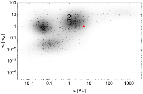
Figure 1: Semi-major axis $a_{1}$ vs. mass ratio $m_{1}$ of 1796 exo-planets (source www.exoplanets.eu). Dark regions, like those labeled 1 and 2, indicate high density regimes; the red dot denotes Jupiter.

3 Resonant variables and averaged equations of motion

Following Brown and Shook (1964), we write the potential, taking the star as origin of the coordinates’ frame:

$$U_{grav}=-\frac{\mu_{*}}{r}-\mu_{1}\big{(}\frac{1}{\Delta}-\frac{1}{r}-\frac{\vec{r}\cdot\vec{r}_{1}}{r_{1}^{3}}\big{)}\ .$$ (4)

Let us denote by $a$, $e$, $i$, $\omega$, $\Omega$, $M$ the standard orbital elements of the third body, where $a$ is the semimajor axis, $e$ the eccentricity, $i$ the orbital inclination, $\omega$ the argument of perihelion, $\Omega$ the longitude of the ascending node, $M$ the mean anomaly. We denote by $a_{1}$, $e_{1}$, $i_{1}$, $\omega_{1}$, $\Omega_{1}$, $M_{1}$ the Keplerian elements of the secondary body. In this work we consider a 1:1 mean motion resonance, which occurs whenever the mean motions of the third and secondary bodies are equal (equivalently, the periods of revolution are equal).

We first introduce the resonant angles in terms of the conservative set-up ($\beta=0$). Precisely, close to the 1:1 MMR, the resonant angle, say $p$, is defined as the difference of the mean orbital longitudes of the third and secondary bodies:

$$p=\lambda-\lambda_{1}\ ,$$

where $\lambda=M+\tilde{\omega}$ with $\tilde{\omega}=\omega+\Omega$, and similarly for $\lambda_{1}$. We denote by $a_{c}$ the value of the semi-major axis of the small body at the 1:1 MMR. In terms of the semi-major axis of the secondary, the value of $a_{c}$ within the conservative framework turns out to be

$$a_{c}=a_{1}\ .$$

We also remark that the term which corresponds to the solar radiation pressure (i.e., (2) with $\gamma=0$) just contributes to modify the mass parameter of the central body, $\mu_{0}$, by the factor $(1-\beta)$. This implies that we have an apparent central mass $\mu_{0}(1-\beta)$, instead of the mass $\mu_{0}$ in the equations of motion for the third body. Therefore, for $\beta\neq 0$ the resonant value of the semi-major axis, in case of a MMR, is shifted according to the following relation:

$$a_{res}=(1-\beta)^{1/3}a_{c}\ ,$$

where $a_{c}$ is the nominal value of the semi-major axis of the conservative case with $\beta=0$.

Let us denote by $(L,G,H,\ell,g,h)$ the action–angle Delaunay’s variables, which are related to the orbital elements by (remind that $\mu_{*}=\mu_{0}+\mu_{1}=1$)

$$L = \sqrt{a}\ ,\qquad\ \ G=\sqrt{a(1-e^{2})}\ ,\qquad\ H=\sqrt{a(1-e^{2})}\ \cos i\ ,$$

$$\ell = M\ ,\qquad\ \ \ g=\omega\ ,\qquad\qquad\qquad\ \ \ \ h=\Omega\ .$$

Setting $s=\sin{i\over 2}$, we have that the elements describing the orbit can be expressed in terms of the Delaunay variables as

$$a={L^{2}}\ ,\qquad e=\sqrt{1-{G^{2}\over L^{2}}}\ ,\qquad s={1\over\sqrt{2}}\ \sqrt{1-{H\over G}}\ .$$ (5)

The Hamiltonian function associated to the restricted three–body problem, and expressed in Delaunay variables, is given by

$${\mathcal{H}}(L,G,H,\ell,g,h,\ell_{1})=-{(1-\beta\mu_{0})^{2}\over{2L^{2}}}-\mu_{1}\ {\mathcal{R}}(L,G,H,\ell,g,h,\ell_{1})\ ,$$ (6)

where $\ell_{1}$ denotes the mean anomaly of the perturber, $\mu_{1}$ is the mass–ratio of the primaries and the perturbing function ${\mathcal{R}}$ is given by the following expression (compare with (4)):

$${\mathcal{R}}={1\over{(r^{2}+r_{1}^{2}-2rr_{1}\cos\psi)^{1\over 2}}}-{{r\cos\psi}\over{r_{1}^{2}}}-{1\over r}\ ,$$ (7)

where $\psi$ is the angle between $(r,r_{1})$. We expand $\mathcal{R}$ around $\rho=r/r_{1}-1$ that gives to low orders (see Lhotka (2014), Appendix B for higher order expansions):

$${\mathcal{R}} \simeq {-\frac{1}{r}}-\frac{21r^{2}\cos^{2}(\psi)}{64\sqrt{2}r_{1}^{3}}-\frac{3r^{2}\cos(\psi)}{16\sqrt{2}r_{1}^{3}}+\frac{r^{2}}{8\sqrt{2}r_{1}^{3}}+\frac{15r\cos^{2}(\psi)}{32\sqrt{2}r_{1}^{2}}$$

$$+ \frac{15\cos^{2}(\psi)}{64\sqrt{2}r_{1}}+\frac{r\cos(\psi)}{8\sqrt{2}r_{1}^{2}}-\frac{r\cos(\psi)}{r_{1}^{2}}+\frac{9\cos(\psi)}{16\sqrt{2}r_{1}}-\frac{3r}{4\sqrt{2}r_{1}^{2}}+{O\left(\rho^{3},\cos^{3}(\psi)\right)}\ .$$

In the next step, the quantities $r$, $r_{1}$, $\psi$ must be expressed in terms of the Delaunay variables by standard Keplerian relations (see, e.g., Celletti (2010); Dvorak and Lhotka (2013)). As a consequence, the perturbing function ${\mathcal{R}}$ can be suitably expanded in Fourier–Taylor series, as shown in Appendix B. We are now in the position to introduce the resonant variables $(P,Q,{W},p,q,{w})$ as

$$P = L\qquad\qquad\qquad\ p=\ell-\ell_{1}+g-g_{1}+h-h_{1}$$

$$Q = G-L\qquad\qquad\ q=g-g_{1}+h-h_{1}$$

$${W} = H-G\qquad\qquad{w}=h-h_{1}$$ (9)

with inverse transformation

$$L = P\qquad\qquad\qquad\qquad\ell=p-q+\ell_{1}$$

$$G = P+Q\qquad\qquad\qquad g=q-{w}+g_{1}$$

$$H = P+Q+{W}\qquad\qquad h={w}+h_{1}\ .$$ (10)

Let us denote by $\overline{\mathcal{R}}$ the average of ${\mathcal{R}}$ over the mean anomaly $\ell_{1}$. Then, the averaged equations in terms of the resonant variables are given by

$$\dot{P} = \mu_{1}{{\partial{\overline{\mathcal{R}}}}\over{\partial p}}\ \qquad\qquad\dot{p}={{(1-\beta\mu_{0})^{2}}\over P^{3}}-1-\mu_{1}{{\partial{\overline{\mathcal{R}}}}\over{\partial P}}$$

$$\dot{Q} = \mu_{1}{{\partial{\overline{\mathcal{R}}}}\over{\partial q}}\ \qquad\qquad\dot{q}=-\mu_{1}{{\partial{\overline{\mathcal{R}}}}\over{\partial Q}}$$

$$\dot{{W}} = \mu_{1}{{\partial{\overline{\mathcal{R}}}}\over{\partial{{w}}}}\ \qquad\qquad\dot{{w}}=-\mu_{1}{{\partial{\overline{\mathcal{R}}}}\over{\partial{{W}}}}\ .$$ (11)

The term -1 in $\dot{p}$ stems from the fact that the transformation (3) depends on time through $\ell_{1}$, appearing in the definition of $p$. Equations (3) represent the contribution of the conservative part to which we must add the effect of the dissipation due to the Poynting–Robertson drag. Precisely, we add the dissipation averaged over the mean anomaly. Since the average dissipation is zero for the angle variables (see Jancart and Lemaitre (2001)), the Poynting–Robertson effect contributes to the equations (3) only by modifying the equations of the action variables according to the following formulae:

$$\dot{P} = \mu_{1}{{\partial{\overline{\mathcal{R}}}}\over{\partial p}}+Y_{P}\ \qquad\qquad\dot{p}={{(1-\beta\mu_{0})^{2}}\over P^{3}}-1-\mu_{1}{{\partial{\overline{\mathcal{R}}}}\over{\partial P}}$$

$$\dot{Q} = \mu_{1}{{\partial{\overline{\mathcal{R}}}}\over{\partial q}}+Y_{Q}\ \qquad\qquad\dot{q}=-\mu_{1}{{\partial{\overline{\mathcal{R}}}}\over{\partial Q}}$$

$$\dot{{W}} = \mu_{1}{{\partial{\overline{\mathcal{R}}}}\over{\partial{{w}}}}+{Y_{W}}\ \qquad\qquad\dot{{w}}=-\mu_{1}{{\partial{\overline{\mathcal{R}}}}\over{\partial{{W}}}}\ ,$$ (12)

where

$$Y_{P} = Y_{L}$$

$$Y_{Q} = Y_{G}-Y_{L}$$

$${Y_{W}} = Y_{H}-Y_{G}$$

and $Y_{L}$, $Y_{G}$, $Y_{H}$ are defined as follows. Denoting by $n$ the mean motion of the third body, from Jancart and Lemaitre (2001) we have the following expressions:

$$Y_{L} = -\mu_{0}\beta n{{1+{3\over 2}e^{2}}\over{c(1-e^{2})^{3\over 2}}}$$

$$Y_{G} = -{{\mu_{0}\beta n}\over c}$$

$$Y_{H} = -{{\mu_{0}\beta n}\over c}\cos i\ .$$

The effect of the dissipation on the orbital elements can be evaluated using the expressions (5), computing the time derivative of the orbital elements and inserting (3) and (3) in place of $\dot{L}$, $\dot{G}$, $\dot{H}$. More precisely, we obtain:

$${{da}\over{dt}} = {{2L\dot{L}}}=-{{\sqrt{a}(1+3e^{2})\mu_{0}\beta n}\over{c(1-e^{2})^{3\over 2}}}$$

$${{de}\over{dt}} = {G\over{L^{2}e}}({G\over L}\dot{L}-\dot{G})={{\sqrt{1-e^{2}}\ \mu_{0}\beta n}\over{\sqrt{a}\ e\ c}}-{{(2+3e)\ \mu_{0}\beta n}\over{2\sqrt{a}\ e\ c(1-e^{2})^{1\over 2}}}$$

$${{di}\over{dt}} = -{1\over{G^{2}\sqrt{1-{H^{2}\over G^{2}}}}}(\dot{H}G-H\dot{G})=0$$ (14)

(the last result comes from the fact that $Y_{H}G-HY_{G}=0$, being $H/G=\cos i$).

The above equations show that the sole dissipation drives to circular orbits (i.e., $e=0$), which end up to collide with the primary body (i.e., $a=0$), while no effect is performed on the inclination.

Remark 1.

To evaluate the occurrence of stationary solutions, we can make use of Tisserand criterion (Moulton (1914), notice that the computation is valid for internal, 1:1 or external resonances). Precisely, we start by mentioning that under the solar radiation pressure the Jacobi constant is given by

$$C={{(1-\beta\mu_{0})}\over a}+2\sqrt{(1-\beta\mu_{0})a(1-e^{2})}\ \cos i\ .$$

Recalling the last result in (3), we have that

$${{dC}\over{dt}}=-{{1-\beta\mu_{0}}\over a^{2}}{{da}\over{dt}}+{{(1-\beta\mu_{0})\cos i}\over{2\sqrt{(1-\beta\mu_{0})a(1-e^{2})}}}\ ((1-e^{2}){{da}\over{dt}}-2ae{{de}\over{dt}})\ .$$

Using the first two expressions in (3), we obtain

$${{dC}\over{dt}} = {{\mu_{0}\beta n}\over{c\ a^{3\over 2}\ (1-e^{2})^{3}}}\Big{[}-2a^{3\over 2}(1-e^{2})^{3}\sqrt{1-\mu_{0}\beta}\cos i+(1-e^{2})^{3\over 2}(2+3e^{2})(1-\mu_{0}\beta)\Big{]}$$

$$= {{\mu_{0}\beta n\sqrt{1-\mu_{0}\beta}}\over{c\ a^{3\over 2}\ (1-e^{2})^{3\over 2}}}\Big{[}-2a^{3\over 2}(1-e^{2})^{3\over 2}\ \cos i+(2+3e^{2})\sqrt{1-\mu_{0}\beta}\Big{]}\ .$$

The condition that the Jacobi integral is constant, i.e. $dC/dt=0$, implies in the limit $e=0$ that

$$a^{3\over 2}\ \cos i=\sqrt{1-\mu_{0}\beta}\ .$$ (15)

Given that Kepler’s third law under solar radiation pressure reads as

$$n^{2}a^{3}=(1-\beta\mu_{0})^{4}\ ,$$ (16)

in a 1:1 MMR (i.e., with $n=1$) we have that (15) reduces to

$$\cos i={{n}\over{(1-\mu_{0}\beta)^{3\over 2}}}\ ,$$ (17)

which can be satisfied only if $n\leq(1-\mu_{0}\beta)^{3\over 2}$. As it is well known (Beaugé and Ferraz-Mello (1994)), this implies that stationary solutions in a 1:1 MMR with non-zero eccentricity and inclination can only exhibit temporary trapping.

When $\beta=0$, from (17) we obtain that the Jacobi integral is preserved just for $n\leq 1$, which corresponds to the small particle on an orbit external to that of the secondary (compare with Beaugé and Ferraz-Mello (1994)). When $\beta\not=0$, this condition is modified and only some external orbits can be considered, precisely those satisfying $n\leq(1-\mu_{0}\beta)^{3\over 2}$.

4 Stationary solutions

In order to find stationary solutions of the averaged problem, we look for the equilibrium solutions associated to (3). More precisely, we fix a set of parameters $(\mu_{1},e_{1},s_{1},\beta)$, where $s_{1}=\sin{i_{1}\over 2}$ with $i_{1}$ denoting the inclination of the secondary. We determine a set of initial conditions $(P_{0},Q_{0},{W_{0}},p_{0},q_{0},{w_{0}})$, such that the right hand sides of (3) are identically zero for the selected parameter values. We then back-transform them into the stationary orbital elements $a_{*},e_{*},i_{*},p_{*},q_{*},{w_{*}}$. We notice that in the conservative setting the equilibria $L_{4}$ and $L_{5}$ are mirror symmetric with respect to $\vec{r}_{1}$. Thus, for $\beta=0$ the equilibrium $L_{4}$ that is given by ($a_{*}$, $e_{*}$, $i_{*}$, $+p_{*}$, $+q_{*}$, $+w_{*}$) maps into the equilibrium $L_{5}$ in terms of ($a_{*}$, $e_{*}$, $i_{*}$, $-p_{*}$, $-q_{*}$, $-w_{*}$). Since the derivatives of the perturbing function with respect to the resonant angles introduce the sine function into the right hand sides of (3) for $\dot{P}$, $\dot{Q}$, $\dot{W}$, then a small deviation from $L_{4}$ is symmetrically mapped into a small deviation from $L_{5}$. This provokes that the right hand sides of $\dot{P}$, $\dot{Q}$, $\dot{W}$ in (3) have opposite signs  with respect to the right hand sides evaluations close to $L_{4}$ and viceversa. However, in the dissipative case, mapping small deviations from $L_{4}$ symmetrically into the vicinity of $L_{5}$ does not alter the signs of the dissipative terms (3). Therefore, since for $\beta\neq 0$ the sum of the conservative and dissipative terms must cancel out to fulfill the requirement for the equilibrium $\dot{P}=\dot{Q}=\dot{W}=0$, then the respective terms will not balance themselves in the same way close to $L_{4}$ in comparison to $L_{5}$. Henceforth, we can expect an asymmetry of the equilibria $L_{4}$ and $L_{5}$ in presence of PR-drag. To evaluate the context of the different dimensions of the $6$-dimensional phase space, we perform the calculations in the planar and spatial versions of the circular and elliptic restricted three-body problems. We start with the circular-planar case of Section 4.1, then we let the orbits be inclined as in Section 4.2, we analyze the elliptic-planar case in Section 4.3 and finally we discuss in Section 4.4 the most general model. The different settings are referred to by appropriate acronyms given at the beginning of each section.

4.1 Circular-planar case (CPRTBP)

We assume that the secondary moves on a circular orbit, while the third body may have non-zero eccentricity, and that all bodies move on the same plane. Therefore we set $e_{1},i_{1},i,\Omega=0$ in $\mathcal{R}$ to obtain ${\overline{\mathcal{R}}}$, and we immediately find ${\dot{W}}=0,{\dot{w}}=0$ in the equations of motion (3). We remark that

$$Y_{Q}=Y_{G}-Y_{L}=-{{\mu_{0}\beta n}\over{c}}\Big{(}1-{{1+{3\over 2}e^{2}}\over{(1-e^{2})^{3\over 2}}}\Big{)}\ .$$ (18)

This implies that $Y_{Q}=0$ whenever $\beta=0$ (the usual conservative case) or if $e=0$; thus, in the dissipative setting, if we set $e=0$, we are reduced to find the solution just of the system of equations

$$\dot{P}=0\ ,\qquad\dot{p}=0\ ,$$ (19)

since $\dot{Q}=0$ also in the conservative case, and we cannot solve for $q_{*}$, since the angle $q$ is an ignorable variable also in the dissipative case due to the fact that $e=0$. We thus neglect the equation $\dot{q}=0$. The system of equations (19) only provides the equilibrium solution for the variables $P$ and $p$; in particular, the solution for $P$ gives the equilibrium value of the semi-major axis. In Figure 2 we report the variation of the equilibrium solutions for $a$ and $p$, for different values of $\mu_{1}$, as a function of the parameter $\beta$, which varies in the interval $[0,0.1]$.

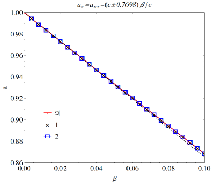
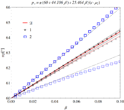
Figure 2: Variation of the equilibrium solutions for $L_{4}$ (dark) and $L_{5}$ (light) in the CPRTBP for $a$ (left) and $p$ (right) as a function of the parameter $\beta$ for different mass parameters $\mu_{1}/\mu_{J}$ equal to $1$ (red dot), $1.5$ (black cross), $0.6$ (blue square), respectively. On the left, $L_{4}$ and $L_{5}$ overlap. Dotted lines correspond to first order formulae.

From Figure 2 we see, that for $\beta=0$ we recover the equilibrium solution of the conservative case at $a_{*}=1$, $p_{*}=60^{\circ}$. For $\beta\not=0$ the equilibrium $a_{*}$ decreases below $0.88$ for all different mass parameters $\mu_{1}$, while the value of the resonant argument $p_{*}$ strongly depends on the choice of $c\cdot\mu_{1}$ (ranging from about $64^{\circ}$ for $\beta=0.1$ and $\mu_{1}=\mu_{J}$ to $66^{\circ}$ for $\beta=0.1$ and $\mu_{1}=0.6\mu_{J}$ for $L_{4}$ and $-62^{\circ}$ to $-63.5^{\circ}$ for $L_{5}$).

4.2 Spatial-circular case (SCRTBP)

In this model we assume that the secondary moves on a circular orbit, the third body may have non-zero eccentricity, and that both smaller bodies move on inclined planes. We thus set $e_{1},\omega_{1}=0$, and keep $i,\Omega\not=0$ in $\mathcal{R}$ to obtain ${\overline{\mathcal{R}}}$. Like in the CPRTBP (see (18)), we find that the equation for $\dot{Q}$ can only be solved for $\beta=0$ or $e=0$ also in the spatial case. However, contrary to the CPRTBP, we have $\dot{W}\not=0$, $\dot{w}\not=0$ in the system of equations (3), and we are led to solve the equations of motion for the variables $P$, $p$, ${W}$, ${w}$, simultaneously. For $a_{*},p_{*}$ we find the same equilibrium values as in the CPRTBP. For $\beta=0$ we recover the known conservative equilibrium value of the Lagrange orbit at $i_{*}=i_{1}$, and ${w}_{*}=0$. The same equilibrium positions are found for $\beta\not=0$: the values for the spatial variables correspond to the case where the two bodies share their lines of nodes, while the relative inclination turns out to be zero. We conclude that the Lagrange orbits in the SCRTBP can be identified with the Lagrange orbits in the CPRTBP to which can be related by simple rotations. However, in the dissipative case we find additional equilibrium solutions, such that the equilibrium inclination $i_{*}$ is different from that of the secondary $i_{1}$ with large ${w}_{*}\not=0$. Since we focus our study on the Lagrange configuration (with ${w}_{*}\simeq 0$), we did not investigate them further. We also remark that an additional class of equilibria can be artificially constructed in the following way. We premise that the solution of the system of equations $\dot{P}=\dot{Q}=\dot{W}=\dot{p}=\dot{q}=\dot{w}=0$ for $i\not=i_{1}$, leads to possible equilibria with very large ${w}$, which is not consistent with the expected physical picture. Instead of solving for all variables, we can fix ${w}=0$ in (3) and solve for the reduced system $\dot{P}=\dot{Q}=\dot{p}=\dot{q}=0$, thus leading to an equilibrium solution $a_{*}$, $e_{*}$, $p_{*}$, $q_{*}$ for $i\not=i_{1}$. It turns out that for a moderate difference of the inclination from $i_{1}$ and for small values of $\beta$, the value of $a_{*}$, $e_{*}$ are not much altered, while a bigger difference is found for $p_{*}$, $q_{*}$, when compared to the case $i=i_{1}$.

When we plot the graphs of the equilibrium solutions for $i_{*}$, ${w}_{*}$, starting for example with $i_{1}=5^{o}$, as a function of the parameter $\beta$, varying in the interval $[0,0.1]$ for different mass ratios $\mu_{1}$, we notice that $i_{*}=i_{1}$, ${w}_{*}=0$ holds true for arbitrary $\beta$. The plots for $a_{*}$, $p_{*}$ overlap to those of Figure 2.

4.3 Elliptic-planar case (EPRTBP)

We assume that the eccentricity of the smaller primary is different from zero, but we make again the assumption that all bodies move on the same plane, like we already did in the CPRTBP. We thus set $i,i_{1},\Omega,\Omega_{1}=0$, but we keep $e,e_{1},g,g_{1}\not=0$ in $\mathcal{R}$ to obtain ${\overline{\mathcal{R}}}$. Like in the CPRTBP we find $(\dot{W}=0,\dot{w}=0)$, also for non-zero $\beta$ in the system (3), and we are thus led to solve a system of equations in the four coordinates $P$, $Q$, $p$, $q$, where we must account for the fact that the dissipation acts only on the action variables $P$ and $Q$.

We find that the correlations between $a_{*}$, $p_{*}$ and $\beta$ remain the same as in the CPRTBP and SCRTBP; we therefore omit the corresponding figures here. We only report in Figure 3 the graphs of the equilibrium solutions for $e_{*}$ and $q_{*}$ as a function of the parameter $\beta$. We find that $e_{*}$ depends on the parameter $\beta$, while we have even a stronger dependency of the equilibrium value for the angle $q_{*}$ with $\beta$. For $\beta=0$ we have $e_{*}=e_{1}$ and $q_{*}=60^{\circ}$. For large enough $\mu_{1}$ the equilibrium $e_{*}$ remains the same, while $q_{*}$ tends to $64^{\circ}$ for $\beta=0.1$. It is interesting to notice that for $\mu_{1}$ small (blue in Figure 3) $e_{*}$ tends to smaller values (still close to $e_{*}=e_{1}$), while the effect on $p_{*}$ is smaller than for larger masses of $\mu_{1}$. We also remark, that while in Figure 2 (right) the solution for $L_{4}$ tends to larger values, in Figure 3 (right) the solution for $L_{5}$ tends to larger ones.

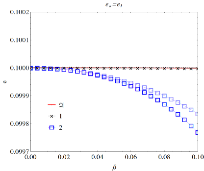
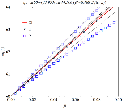
Figure 3: Variation of the equilibrium solutions for $L_{4}$ (dark) and $L_{5}$ (light) in the EPRTBP for $e$ (left), and $q$ (right) as a function of the parameter $\beta$ for $e_{1}=0.1$ and different mass ratios $\mu_{1}/\mu_{J}$ equal $1$ (red dot), $1.5$ (black cross), and $0.6$ (blue square), respectively. The plots for $a$, $p$ coincide with those of Figure 2. On the left $L_{4}$ and $L_{5}$ overlap for $\mu_{J}$ and $1.5\mu_{J}$. Dotted lines correspond to first order formulae.

4.4 Spatial-elliptic case (SERTBP)

In the most general case, we assume that the secondary moves on an elliptic orbit and on an inclined plane, so that both $e_{1}$ and $s_{1}$ are different from zero. We thus investigate the full dynamics of the equations (3), where we keep all orbital elements in $\mathcal{R}$ to obtain ${\overline{\mathcal{R}}}$. For $\beta=0$ we find the real equilibrium solution at $a_{*}=a_{1}=1$, $e_{*}=e_{1}$, $i_{*}=i_{1}$, $p_{*}=q_{*}=60^{\circ}$, and $w_{*}=0$, that corresponds to the well-known Lagrange orbit: the orbital planes share their line of nodes with zero relative inclination, while the line of apsides of the third body is rotated by $60^{\circ}$, and the difference in orbital longitudes is $60^{\circ}$. For $\beta\not=0$ we solve for the system of equations in all variables $(P,Q,{W},p,q,{w})$ and we obtain that the equilibrium solution is typically obtained when $e=e_{1}$ and $s=s_{1}$. Indeed, the equation for $\dot{Q}$ does not depend on $s_{1}$ and it is zero for $e=e_{1}$. On the other hand, the equation for $\dot{W}$ does not depend on $e_{1}$ and it becomes zero only when $s=s_{1}$.

We report in Figure 4 the graphs of the equilibrium solutions for $a$, $e$, $s$, $p$, $q$ and $w$ for different mass parameters $\mu_{1}$ as functions of the parameter $\beta$, varying in the interval $[0,0.1]$.

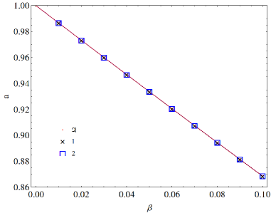
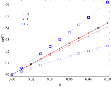
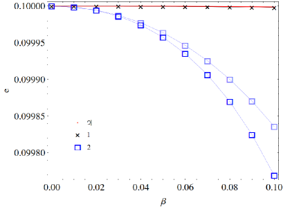
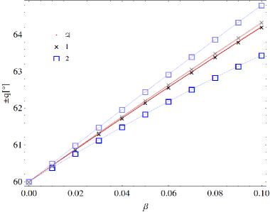
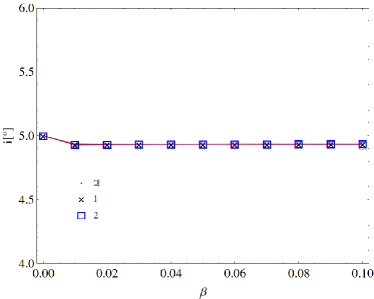
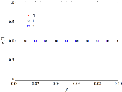
Figure 4: Variation of the equilibrium solutions for $L_{4}$ (dark) and $L_{5}$ (light) in the SERTBP for $e_{1}=0.1$, $i_{1}=5^{\circ}$ and for different mass parameter $\mu_{1}/\mu_{J}$ equal $1$ (red dot), $1.5$ (black cross), $0.6$ (blue square), for $a$ (upper left panel), $p$ (upper right panel), $e$ (middle left panel), $q$ (middle right panel), $i$ (bottom left panel), $w$ (bottom right panel) as functions of the parameter $\beta$. Light curves overlap with dark ones if not visible.

In comparison with Figures 2–3 we find that from a qualitative point of view the correlations of $a,e,p,q$ with $\beta$ at their equilibrium values remain the same. We notice, that in the SERTBP, for $\beta\neq 0$ the inclination $i_{*}$ tends to slightly lower values than $i_{1}=5^{\circ}$ for $w_{*}$ fixed at $0$ degrees. No difference between $L_{4}$ and $L_{5}$ is visible with respect to $i$ and $w$.

We observe in Figures 2-4 that the difference in the locations of the equilibria in the parameter space between the cases Jupiter and case 1 is small ($10^{-2\ o}$ for $p$ and $10^{-3\ o}$ for $q$ with $\beta=0.05$) compared to case 2 ($10^{-1\ o}$ for $p$ and $10^{-2\ o}$ for $q$ with $\beta=0.05$). A possible explanation is as follows: terms in (3) entering proportionally to $\mu_{1}$ need to be balanced with the dissipative terms that enter with proportionality factor $\mu_{0}\beta n/c$. Due to our special choice of units, this term is proportional to $(1-\mu_{1})\beta a_{1}n_{1}\,n$. From Table 1, with $n_{1}=2\pi/P_{1}$, we find that the terms (3) for Jupiter and case 1 are of the same order of magnitude, while for case 2 the corresponding term turns out to be one order of magnitude bigger. We can therefore expect that the deviation of the equilibria from the conservative solution for Jupiter and case 1 are comparable, while the deviation for case 2 is larger.

5 On the behavior of the eigenvalues of the equilibrium positions

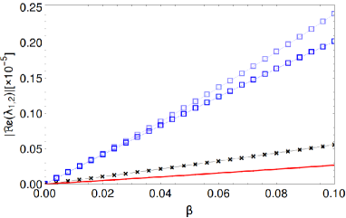
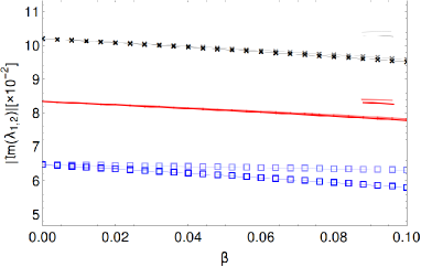
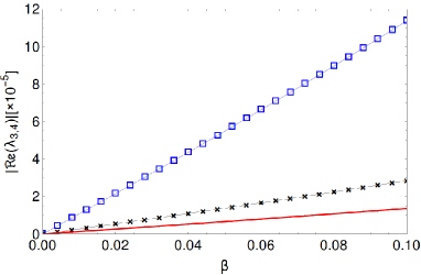
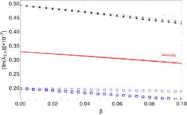
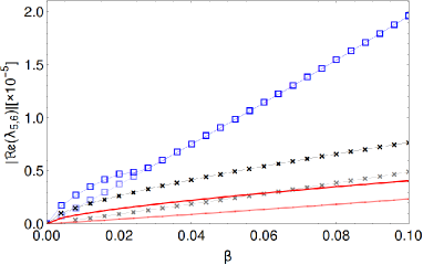
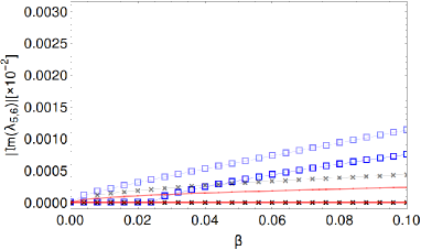
Figure 5: Absolute values of real (left column) and imaginary parts (right column) of $\lambda_{1,2}$ (top row), $\lambda_{3,4}$ (middle row), and $\lambda_{5,6}$ (bottom row) for $e_{1}=0.1$, $i_{1}=5^{o}$ and for different mass parameters $\mu_{1}/\mu_{J}$ equal $1$ (red dot), $1.5$ (black cross), and $0.6$ (blue square) in dependency of the dissipative parameter $\beta$. We show the behaviour close to $L_{4}$ (thick) and $L_{5}$ (thin), respectively.

In this section we investigate the eigenvalues of the linearized averaged vector field (3) in the neighborhood of the equilibrium. Let us consider a small displacement close to the equilibrium, say $(P_{0},Q_{0},{W_{0}},p_{0},q_{0},{w_{0}})$:

$$P = P_{0}+\delta P\ ,\quad Q=Q_{0}+\delta Q\ ,\quad{W=W_{0}+\delta W}$$

$$p = p_{0}+\delta p\ ,\quad\ \ q=q_{0}+\delta q\ ,\quad\ \ \ {w=w_{0}+\delta w}\ .$$ (20)

The linearization around the equilibrium position provides the matrix $A=(a_{ij})$ with elements:

$$a_{1\alpha} = -\mu_{1}\frac{\partial^{2}{\overline{\mathcal{R}}}}{\partial p\partial\alpha}+\frac{\partial Y_{P}}{\partial\alpha}\ ,\quad a_{4\alpha,\alpha\not=1}=\mu_{1}\frac{\partial^{2}{\overline{\mathcal{R}}}}{\partial P\partial\alpha}$$

$$a_{2\alpha} = -\mu_{1}\frac{\partial^{2}{\overline{\mathcal{R}}}}{\partial q\partial\alpha}+\frac{\partial Y_{Q}}{\partial\alpha}\ ,\quad a_{5\alpha}=\mu_{1}\frac{\partial^{2}{\overline{\mathcal{R}}}}{\partial Q\partial\alpha}$$

$$a_{3\alpha} = -\mu_{1}\frac{\partial^{2}{\overline{\mathcal{R}}}}{\partial{{w}}\partial\alpha}+\frac{\partial{{Y_{W}}}}{\partial\alpha}\ ,\quad a_{6\alpha}=\mu_{1}\frac{\partial^{2}{\overline{\mathcal{R}}}}{\partial{{W}}\partial\alpha}$$

with $\alpha=P,Q,{W},p,q,{w}$ and

$$a_{41}=\frac{3(1-\beta\mu_{0})^{2}}{P^{4}}+\mu_{1}\frac{\partial^{2}{\overline{\mathcal{R}}}}{\partial P}\ .$$

We immediately notice that all derivatives of $Y_{P}$ and $Y_{Q}$ with respect to $p$, $q$, $w$, $W$ are zero and that the derivatives of $Y_{W}$ with respect to $p$, $q$, $w$ are zero. The solution of the variational equations

$$\frac{d}{dt}\left(\delta P,\delta Q,\delta{W},\delta p,\delta q,\delta{w}\right)^{\top}=A\cdot\left(\delta P,\delta Q,\delta{W},\delta p,\delta q,\delta{w}\right)^{\top}$$ (21)

contains terms of the form

$$c_{j}{\mathbf{v}}_{j}e^{\lambda_{j}t}\ ,$$

where ($c_{j}$, ${\mathbf{v}}_{j}$, $\lambda_{j}$), $j=1,...,6$, denotes the eigensystem of $A$. We show the stability of the linearized tangent flow on the basis of the eigenvalues $\lambda_{j}$ with $j=1,...,6$ in Figure 5. In the top row we show the dependency of the absolute values of the real and imaginary parts of $\lambda_{1,2}$, related to the linearized dynamics of the pair $(\delta P,\delta p)$, for varying $\beta$ and different mass ratios $\mu_{1}/\mu_{J}$ from Table 1. Our conclusions are as follows:

• For $\beta=0$ the real parts are zero for all mass ratios. With increasing $\beta$ the absolute values of $\lambda_{1,2}$ increase. The slopes are steeper for larger ratios $\beta/c$, indicating less stable motions.

• The absolute values of the imaginary parts, that are related to the fundamental frequencies of motion, decrease with increasing $\beta$, indicating slightly larger periods of oscillation for larger $\beta$. We also observe, that larger $a_{1}$ leads to bigger values of the absolute eigenvalues.

• We demonstrate that the stability close to $L_{4}$ is different from the stability close to $L_{5}$ as already pointed out in Murray (1994) (but based on the CPRTBP and an oversimplified drag model). Maximum differences in absolute values between $L_{4}$ and $L_{5}$ are largest (left: $10^{-7}$, right: $10^{-3}$) for the case $\mu_{1}=0.6$ and much smaller (left: $10^{-9}$, right: $10^{-4}$) for the cases $\mu_{1}=1,1.5$.

Next, we investigate the linearized stability of motion of the dynamics related to the pair of variables $(\delta Q,\delta q)$, see middle row of Figure 5:

• The qualitative behaviour, w.r.t. $\beta$, $\mu_{1}$, and $a_{1}$, of the dynamics of the absolute values of the real and imaginary parts of $\lambda_{3,4}$ is the same as for the pair $\lambda_{1,2}$.

• Instabilities induced in the dynamics of the pair $(\delta Q,\delta q)$ are 100 orders of magnitude stronger than instabilities induced in the dynamics of the pair $(\delta P,\delta p)$.

• The maximal differences in absolute values between $L_{4}$ and $L_{5}$ are of the order of magnitude of $10^{-9}$ for $\mu_{1}=1,1.5$ and $10^{-7}$ for the case $\mu_{1}=0.6$.

Finally, we find from Figure 5 (bottom row):

• The main difference in the linearized motions related to the pair $(\delta{W},\delta{w})$ w.r.t. the previous cases is the increase in oscillation frequency for larger $\beta$ (see bottom, right).

• The maximum differences in absolute values between $L_{4}$ and $L_{5}$ are of the order of $10^{-6}$ for the cases $\mu_{1}=0.6,1,1.5$.

As a conclusion, due to the presence of non-zero real parts in all pairs of eigenvalues $\lambda_{i,i+1}$ with $i=1,3,5$, we find an exponential divergence in the solution of (21); therefore, our system does not provide spectral or linear stability.

We also notice that the distance of the equilibria in the parameter space for $\beta\neq 0$ from the conservative solution is larger for smaller mass ratios, and that the difference between $L_{4}$ and $L_{5}$ is due to the asymmetry of nearby initial conditions - the effect being larger for smaller masses (see further explanations at the beginning and end of Section 4). Moreover, the stability is mainly affected by the semi-major axis of the perturber: indeed, smaller values of $a_{1}$ indicate higher velocities and thus stronger drag terms, that lead to less stable motions, which correspond to larger absolute values of the real parts in consistency with Figure 5.

Finally, we add a remark on the effect of the dissipative parameter $\beta$ on the symplectic phase space structure. If we denote by $J$ the $6\times 6$ symplectic matrix, it holds for $A$ that:

$$|\max_{i,j}(A^{\top}J+JA)_{i,j}|=d_{0}\ ,$$ (22)

with the maximum computed over all elements of the matrix $A^{\top}J+JA$ and with $d_{0}=0$ only for $\beta=0$. At first order in $\beta$ we find

$$d_{0}=\frac{\beta}{c}\cdot\frac{7-6e_{0}^{2}+\sin^{2}(i_{0}/2)}{\sqrt{a_{0}(1-e_{0}^{2})}}+O(\beta^{2})\ ,$$ (23)

that is proportional to the ratio $\beta/c$ in the same way as the slopes in the absolute values of the real parts in Figure 5. We also notice, that for $\beta=0$ the sum of the conjugated eigenvalues of $A$ turns out to be zero, because for $\beta=0$ the matrix $A$ becomes an infinitesimally symplectic matrix. However, for $\beta\not=0$ we find

$$d_{1} = |\lambda_{1}+\lambda_{2}|=O(\beta^{2})$$

$$d_{2} = |\lambda_{3}+\lambda_{4}|=|\frac{\beta}{c}\cdot\frac{6(e_{0}^{2}-1)}{\sqrt{a_{0}}}|+O(\beta^{2})$$

$$d_{3} = |\lambda_{5}+\lambda_{6}|=|\frac{\beta}{c}\cdot\frac{1}{\sqrt{a_{0}(1-e_{0}^{2})}}|+O(\beta^{2})\ .$$ (24)

We remark that, up to first order in $\beta$, the $d_{i}$’s do not depend on the mass ratio $\mu_{1}$. We provide in Figure 6 the dependency of $d_{i}$ versus $\beta$; the left plot is based on our first order formulae (22)–(5), the right plot shows the $d_{i}$’s obtained as follows. We calculate the equilibrium values $P_{0},Q_{0},{W_{0}},p_{0},q_{0},{w_{0}}$ from (3) for $\mu_{1}=\mu_{J}$, $e_{1}=0.1$, $i_{1}=5^{\circ}$. Next, we expand the averaged vector field around the equilibrium to obtain a numerical value for $A$. Finally, we implement the formula $|\max_{i,j}(A^{\top}J+JA)_{i,j}|=d_{0}$, $|\lambda_{1}+\lambda_{2}|$, $|\lambda_{3}+\lambda_{4}|$, $|\lambda_{5}+\lambda_{6}|$ to obtain the $d_{i}$’s in a purely numerical way. As we can see comparing the two plots of Figure 6, the first order formulae reproduce quite well the values of the infinitesimally symplectic parameter $d_{0}$ as well as the values of $d_{1}$, $d_{2}$, $d_{3}$.

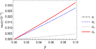
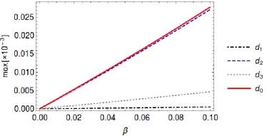
Figure 6: Comparison of the first order formulae (23)-(5) on the left with the numerically obtained figure on the right for $\mu_{1}=\mu_{J}$, $e=e_{1}$, $i_{1}=5^{\circ}$.

6 Numerical study based on the unaveraged model

In this section we perform a numerical survey to confirm our results by comparing the analysis of the averaged model with the unaveraged equations of motion. For this reason we integrate (3) using a Runge-Kutta 4-th order integration method with initial conditions that define the equilibrium of the averaged dynamics. We integrate the initial conditions as long $\psi$ (the angle between $\vec{r}_{1}$ and $\vec{r})$ stays within the interval $[10^{\circ},180^{\circ}]$, with a maximum integration time set to $T=600\,000$ revolution periods of the secondary. Since our starting values are obtained from an averaged model, we expect a slight shift with respect to the non-averaged model. Moreover, the equilibrium of the averaged dynamics corresponds to a periodic orbit of the un-averaged system, that explicitely depends on time $t$ through the perturbing planet. For the Lagrange orbit associated to $L_{4}$, $L_{5}$ in the SERTBP, we expect for $\beta=0$ that $a$, $e$, $i$ stay constant, while the resonant angles $p$, $q$ oscillate around $60^{\circ}$, and the angle $w$ oscillates around $0^{\circ}$, respectively. For small $\beta$, say $\beta=0.01$ and different $\mu_{1}$, we get a libration of $a$, $p$, $e$, $q$ in Figure 7, and an oscillation of $i$, $w$ around the initial values. For some orbital elements, most notably semimajor axis and inclination, we observe a small shift between the averaged motion, that we predicted from averaging theory in Section 4, and the mean value, around which the elements oscillate, in the unaveraged dynamics.

We are left to confirm our prediction of Section 5, that dissipative effects act on time-scales proportional to the ratio $\beta/c$, that is proportional to the quantity $\beta\,a_{1}\,n_{1}$ in arbitrary units: from Figure 7 we roughly estimate the ratios of the times of temporary stability between the Jupiter-like case (red) and case 1 (black) to be about $2$, and between case 1 and case 2 to be about $4$, that is in perfect agreement with the values of $\beta\,a_{1}\,n_{1}$ that we may calculate from Table 1. We conclude our numerical survey with a study of the libration width of the elements $p$ and $a$ in dependency of the parameter $\beta$. We show in Figure 8 the evolution in time of the elements $a$ (left) and $p$ (right) for $\beta\in[0.01,0.05]$. As we can see, for larger values of $\beta$ the element $p$ leaves the librational resonance earlier, as we already predicted from averaging theory.

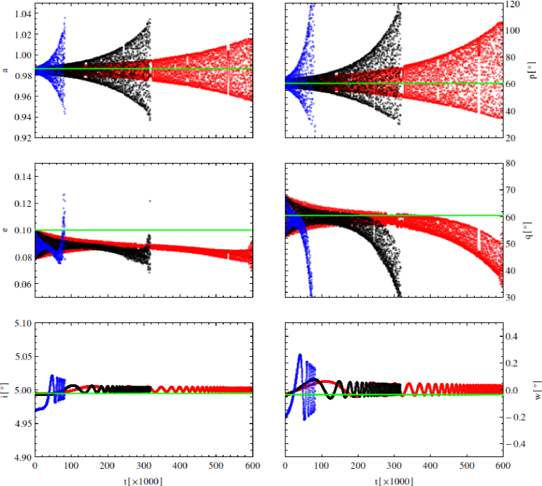
Figure 7: Lagrange orbit for $\mu_{1}/\mu_{J}$ equal $1$ (red), $1.5$ (black), and $0.6$ (blue) for $e_{1}=0.1$, $i_{1}=5^{\circ}$, and $\beta=0.01$. Initial conditions coincide with the equilbria of the averaged system (green thick): $a(0)\simeq 0.98$, $e(0)\simeq 0.99$, $i(0)\simeq 4.99$, $p(0)\simeq 60.42^{\circ}$, $q(0)\simeq 60.44^{\circ}$, and ${w}(0)\simeq 0$.

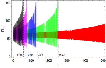
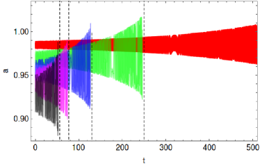
Figure 8: The effect of $\beta$ on the time of temporary stability of Lagrange orbits for $\mu_{1}=\mu_{J}$, $e=e_{1}$, $i=5^{\circ}$: $0.01$ (red), $0.02$ (green), $0.03$ (blue), $0.04$ (magenta), and $0.05$ (black).

7 Summary and conclusions

We investigated the Poynting-Robertson (PR) effect on the co-orbital resonant motion of dust-sized particles with a planet in the framework of several models, from the circular-planar case to the spatial-elliptic restricted three-body problem. Our study is based on a simplified resonant model that we derived on the basis of the equations of motion averaged over the mean anomaly of the perturbing planet. We use the resonant model to find the variation of the equilibrium solution in the orbital element space of the small particle for different particle size and mass parameters. We only find temporary stability of the Lagrange type orbits in presence of PR drag forces, and show by linear stability analysis that the instability is due to the steadily increase of the libration width of the main resonant angle. Our results are validated in several different models of increasing complexity, and they are confirmed on the basis of a detailed numerical survey of the unaveraged equations of motion.

The main results of our study are described below.

• Stable motion for dust sized particles is not possible due to Poynting-Robertson effect.

• Temporary stability of particles displaying a tadpole motion in the non-averaged system occurs for a wide range of parameters and initial conditions.

• The 1:1 resonance with a planet allows a temporary capture of dust size particles also within the orbit of the perturbing planet, provided it is still in resonance - a fact that has been overseen by previous studies that found that resonant capture of dust size particles for inner resonances is not possible due to PR drag.

• We confirm the presence of a possible asymmetry of the stability indices of $L_{4}$ and $L_{5}$ also in the SERTBP, using a more realistic force model, than it was used in Murray (1994) and based on the CPRTBP.

A proper expansion of the perturbing function allows us to treat the problem by means of averaging theory. The extension of our work to the spatial, elliptic, restricted three-body (SERTBP) problem shows the importance of the third dimension in this kind of studies. Inner and outer resonances should therefore be reinvestigated in the framework of the SERTBP. The effect of dissipative forces on the resonant motion may play a key role in planetary formation processes. Finally, it would be interesting to investigate the effect of other dissipative forces on resonant motions.

Acknowledgments

A.C. was partially supported by PRIN-MIUR 2010JJ4KPA$\_$009, GNFM-INdAM and by the European Grant MC-ITN Stardust. C. L. was financially supported by the Austrian Science Fund (FWF) project J-3206.

Appendix A Basic series expansions used in our study, based on Stumpff (1959)

Let $J_{k}$ be the Bessel function of the first kind. The radius $r$ (similar $r_{1}$) and its inverse $r^{-1}$ (and $r_{1}^{-1}$) can be obtained from:

$$\frac{r}{a} = 1+\frac{1}{2}e^{2}-2e\sum_{k=1}^{\infty}\frac{dJ_{k}(ke)}{de}\frac{\cos(kM)}{k^{2}}$$

$$\frac{a}{r} = 1+2\sum_{k=1}^{\infty}J_{k}(ke)\cos(kM)\ .$$

The cosine and sine of the true anomaly $f$ are given by:

$$\cos(f) = -e+2\frac{1-e^{2}}{e}\sum_{k=1}^{\infty}J_{k}(ke)\cos(kM)\ ,$$

$$\sin(f) = 2\sqrt{1-e^{2}}\sum_{k=1}^{\infty}\frac{dJ_{k}(ke)}{de}\frac{\sin(kM)}{k}\ .$$

Let us denote by $\xi$, $\eta$, $\zeta$ the position of a celestial body in the orbital frame (where $\zeta=0$). In this setting we have

$$\frac{\xi}{a} = -\frac{3}{2}e+2\sum_{k=1}^{\infty}\frac{dJ_{k}(ke)}{de}\frac{\cos(kM)}{k^{2}}\ ,$$

$$\frac{\eta}{a} = 2\frac{\sqrt{1-e^{2}}}{e}\sum_{k=1}^{\infty}J_{k}(ke)\frac{\sin(kM)}{k}\ .$$

Time derivatives $\dot{r}$, $\dot{\xi}$, $\dot{\eta}$, $\dot{\zeta}$ can be directly obtained from $d/dt$ (assuming $M=nt$):

$$\frac{\dot{r}}{a} = 2ne\sum_{\nu=1}^{\infty}\frac{dJ_{\nu}(\nu e)}{de}\frac{\sin(M)}{\nu}\ ,$$

$$\frac{\dot{\xi}}{a} = -2n\sum_{k=1}^{\infty}\frac{dJ_{k}(ke)}{de}\frac{\sin(kM)}{k}\ ,$$

$$\frac{\dot{\eta}}{a} = 2n\frac{\sqrt{1-e^{2}}}{e}\sum_{k=1}^{\infty}J_{k}(ke)\cos(kM)\ ,\ .$$

The transformation to the inertial reference frame is given by the rotation matrix $R_{M}=R_{3}(\Omega)R_{1}(i)R_{3}(\omega)$, where $R_{i}$ denotes the rotation around the $i$-th axis ($x$, $y$, $z$). Using the notation $c_{\#}=\cos(\#)$, $s_{\#}=\sin(\#)$ we find:

$$R_{M}=\left(\begin{array}[]{ccc}c_{\omega}c_{\Omega}-c_{i}s_{\omega}d_{\Omega}&s_{\omega}-c_{\Omega}-c_{i}c_{\omega}s_{\Omega}&s_{i}s_{\Omega}\\ c_{i}s_{\omega}c_{\Omega}+c_{\omega}s_{\Omega}&c_{i}c_{\omega}c_{\Omega}-s_{\omega}s_{\Omega}&s_{i}-c_{\Omega}\\ s_{i}s_{\omega}&s_{i}c_{\omega}&c_{i}\\ \end{array}\right).$$

Appendix B Equilateral perturbing function

We start from the expression of ${\mathcal{R}}$ given in (7). Using the small parameter $\rho=\frac{r}{r_{1}}-1$, the distance $\Delta^{-1}$ becomes in terms of $\rho$:

$$\frac{1}{\Delta}=\frac{1}{r_{1}}\frac{1}{\sqrt{A+A\rho+\rho^{2}}}\ .$$

with $A=2\left(1-\cos\psi\right)$. Setting $\epsilon=\rho+\frac{\rho^{2}}{A}$ we find

$${\frac{1}{\Delta}}=\frac{1}{r_{1}}\frac{1}{\sqrt{2}}\frac{1}{\sqrt{1-\cos\psi}}\frac{1}{\sqrt{1+\epsilon}}\ ,$$

provided $|\cos\psi|<1$, $|\epsilon|<1$; the expansion of $\Delta^{-1}$ becomes

$$\Delta^{-1}\simeq\frac{1}{\sqrt{2}}\frac{1}{r_{1}}\sum_{j=0}^{\infty}{\left(-1\right)^{j}\left(\begin{array}[]{c}-1/2\\ j\\ \end{array}\right)\cos(\psi)^{j}}\sum_{n=0}^{\infty}\left(\begin{array}[]{c}-1/2\\ n\\ \end{array}\right)\epsilon^{n}\ ,$$

and the expansion of the perturbing function, valid close to $r/r_{1}\simeq 1$, is given by

$${\mathcal{R}}=\frac{1}{\sqrt{2}}\frac{1}{r_{1}}\sum_{j=0}^{\infty}{\left(-1\right)^{j}\left(\begin{array}[]{c}-1/2\\ j\\ \end{array}\right)\cos(\psi)^{j}}\sum_{n=0}^{\infty}\left(\begin{array}[]{c}-1/2\\ n\\ \end{array}\right)\epsilon^{n}-\frac{r\cos\psi}{r_{1}^{2}}{-\frac{1}{r}}\ .$$

If we compute the expansion up to the order $2$ in $\rho$ and order $2$ in $\cos\psi$, we get the expression (3). Setting $\alpha=a/a_{1}-1$, $\cos i=1-s^{2}$, $\sin i=2s$, $\lambda=M+\tilde{\omega}$, $\tilde{\omega}=\omega+\Omega$ (and analogously for $s_{1}$, $\lambda_{1}$, $\tilde{\omega}_{1}$), and using standard series expansions for $r$, $r_{1}$, and $\cos(\psi)$ we find:

$${\frac{1}{r}}+a_{1}{\mathcal{R}}=-\frac{10\alpha^{2}+152\alpha+112}{256\sqrt{2}}-\frac{\left(15\alpha^{2}+96\alpha+81\right)e^{2}}{256\sqrt{2}}-$$

$$\frac{3\left(5\alpha^{2}+32\alpha+27\right)e_{1}^{2}}{256\sqrt{2}}-\frac{\left(-84\alpha^{2}-48\alpha+96\right)s^{2}}{256\sqrt{2}}+\frac{3\left(7\alpha^{2}+4\alpha-8\right)s_{1}^{2}}{64\sqrt{2}}$$

$$+\left(\frac{5\alpha^{2}}{64\sqrt{2}}+\frac{43\alpha}{64\sqrt{2}}+\frac{19}{32\sqrt{2}}\right)e\cos\left(\lambda-\tilde{\omega}\right)$$

$$+\cos\left(\lambda-\lambda_{1}\right)\bigg{(}-\frac{3\alpha^{2}}{16\sqrt{2}}+\left(-1-\frac{1}{4\sqrt{2}}\right)\alpha$$

$$+\left(-\frac{3\alpha^{2}}{32\sqrt{2}}+\left(\frac{1}{2}-\frac{1}{4\sqrt{2}}\right)\alpha-\frac{23}{32\sqrt{2}}+\frac{1}{2}\right)e^{2}$$

$$+\left(-\frac{3\alpha^{2}}{32\sqrt{2}}+\left(\frac{1}{2}-\frac{1}{4\sqrt{2}}\right)\alpha-\frac{23}{32\sqrt{2}}+\frac{1}{2}\right)e_{1}^{2}$$

$$+\left(\frac{3\alpha^{2}}{16\sqrt{2}}+\left(1+\frac{1}{4\sqrt{2}}\right)\alpha-\frac{1}{2\sqrt{2}}+1\right)s^{2}$$

$$+\left(\frac{3\alpha^{2}}{16\sqrt{2}}+\left(1+\frac{1}{4\sqrt{2}}\right)\alpha-\frac{1}{2\sqrt{2}}+1\right)s_{1}^{2}+\frac{1}{2\sqrt{2}}-1\bigg{)}$$

$$+\left(-\frac{21\alpha^{2}}{32\sqrt{2}}-\frac{3\alpha}{8\sqrt{2}}+\frac{3}{4\sqrt{2}}\right)ss_{1}\cos\left(\Omega-\Omega_{1}\right)$$

$$+\left(\frac{3\alpha^{2}}{16\sqrt{2}}+\frac{3\alpha}{8\sqrt{2}}+\frac{15}{32\sqrt{2}}\right)ee_{1}\cos\left(\tilde{\omega}-\tilde{\omega}_{1}\right)$$

$$+\left(-\frac{3\alpha^{2}}{32\sqrt{2}}-\frac{3\alpha}{16\sqrt{2}}-\frac{3}{8\sqrt{2}}\right)e_{1}\cos\left(\lambda-\tilde{\omega}_{1}\right)$$

$$+\left(\frac{3\alpha^{2}}{8\sqrt{2}}+\left(\frac{3}{2}+\frac{9}{16\sqrt{2}}\right)\alpha-\frac{3}{8\sqrt{2}}+\frac{3}{2}\right)e\cos\left(\tilde{\omega}-\lambda_{1}\right)$$

$$+\left(-\frac{15\alpha^{2}}{128\sqrt{2}}-\frac{81\alpha}{64\sqrt{2}}-\frac{33}{32\sqrt{2}}\right)e_{1}\cos\left(\lambda_{1}-\tilde{\omega}_{1}\right)$$

$$+\left(-\frac{15\alpha^{2}}{128\sqrt{2}}+\left(-\frac{1}{8}-\frac{7}{32\sqrt{2}}\right)\alpha-\frac{11}{64\sqrt{2}}-\frac{1}{8}\right)e^{2}\cos\left(-2\tilde{\omega}+\lambda+\lambda_{1}\right)$$

$$+\left(-\frac{3\alpha^{2}}{16\sqrt{2}}+\left(-1-\frac{1}{4\sqrt{2}}\right)\alpha+\frac{1}{2\sqrt{2}}-1\right)s^{2}\cos\left(\lambda+\lambda_{1}-2\Omega\right)$$

$$+\left(\frac{63\alpha^{2}}{128\sqrt{2}}+\frac{51\alpha}{128\sqrt{2}}-\frac{21}{64\sqrt{2}}\right)e\cos\left(\tilde{\omega}+\lambda-2\lambda_{1}\right)$$

$$+\left(-\frac{3\alpha^{2}}{16\sqrt{2}}+\left(-1-\frac{1}{4\sqrt{2}}\right)\alpha+\frac{1}{2\sqrt{2}}-1\right)s_{1}^{2}\cos\left(\lambda+\lambda_{1}-2\Omega_{1}\right)$$

$$+\left(-\frac{3\alpha^{2}}{8\sqrt{2}}+\left(-2-\frac{1}{2\sqrt{2}}\right)\alpha+\frac{1}{\sqrt{2}}-2\right)ss_{1}\cos\left(\lambda-\lambda_{1}-\Omega+\Omega_{1}\right)$$

$$+\left(\frac{21\alpha^{2}}{32\sqrt{2}}+\frac{3\alpha}{8\sqrt{2}}-\frac{3}{4\sqrt{2}}\right)ss_{1}\cos\left(-2\lambda_{1}+\Omega+\Omega_{1}\right)$$

$$+\left(\frac{3\alpha^{2}}{8\sqrt{2}}+\left(2+\frac{1}{2\sqrt{2}}\right)\alpha-\frac{1}{\sqrt{2}}+2\right)ss_{1}\cos\left(\lambda+\lambda_{1}-\Omega-\Omega_{1}\right)$$

$$+\left(-\frac{15\alpha^{2}}{128\sqrt{2}}+\left(-\frac{1}{8}-\frac{7}{32\sqrt{2}}\right)\alpha-\frac{11}{64\sqrt{2}}-\frac{1}{8}\right)e_{1}^{2}\cos\left(-2\tilde{\omega}_{1}+\lambda+\lambda_{1}\right)$$

$$+\left(\frac{15\alpha^{2}}{128\sqrt{2}}+\frac{3\alpha}{4\sqrt{2}}+\frac{81}{128\sqrt{2}}\right)ee_{1}\cos\left(-\tilde{\omega}+\tilde{\omega}_{1}+\lambda-\lambda_{1}\right)$$

$$+\left(\frac{15\alpha^{2}}{16\sqrt{2}}+\left(3+\frac{3}{2\sqrt{2}}\right)\alpha-\frac{9}{32\sqrt{2}}+3\right)ee_{1}\cos\left(\tilde{\omega}+\tilde{\omega}_{1}-2\lambda_{1}\right)$$

$$+\left(-\frac{15\alpha^{2}}{32\sqrt{2}}+\left(-2-\frac{11}{16\sqrt{2}}\right)\alpha+\frac{5}{8\sqrt{2}}-2\right)e_{1}\cos\left(\tilde{\omega}_{1}+\lambda-2\lambda_{1}\right)$$

$$+\left(\frac{15\alpha^{2}}{128\sqrt{2}}+\frac{3\alpha}{4\sqrt{2}}+\frac{81}{128\sqrt{2}}\right)ee_{1}\cos\left(-\tilde{\omega}-\tilde{\omega}_{1}+\lambda+\lambda_{1}\right)$$

$$+\left(-\frac{63\alpha^{2}}{256\sqrt{2}}+\frac{3\alpha}{32\sqrt{2}}+\frac{177}{256\sqrt{2}}\right)ee_{1}\cos\left(\tilde{\omega}-\tilde{\omega}_{1}+\lambda-\lambda_{1}\right)$$

$$+\left(\frac{5\alpha^{2}}{256\sqrt{2}}+\frac{19\alpha}{64\sqrt{2}}+\frac{71}{256\sqrt{2}}\right)e^{2}\cos\left(2\lambda-2\tilde{\omega}\right)$$

$$+\left(-\frac{21\alpha^{2}}{64\sqrt{2}}-\frac{3\alpha}{16\sqrt{2}}+\frac{3}{8\sqrt{2}}\right)s^{2}\cos(2\lambda-2\Omega)$$

$$+\cos\left(2\lambda-2\lambda_{1}\right)\bigg{(}-\frac{21\alpha^{2}}{128\sqrt{2}}-\frac{3\alpha}{32\sqrt{2}}+\left(\frac{105\alpha^{2}}{256\sqrt{2}}-\frac{225}{256\sqrt{2}}\right)e^{2}$$

$$+\left(\frac{105\alpha^{2}}{256\sqrt{2}}-\frac{225}{256\sqrt{2}}\right)e_{1}^{2}+\left(\frac{21\alpha^{2}}{64\sqrt{2}}+\frac{3\alpha}{16\sqrt{2}}-\frac{3}{8\sqrt{2}}\right)s^{2}$$

$$+\left(\frac{21\alpha^{2}}{64\sqrt{2}}+\frac{3\alpha}{16\sqrt{2}}-\frac{3}{8\sqrt{2}}\right)s_{1}^{2}+\frac{3}{16\sqrt{2}}\bigg{)}$$

$$+\left(-\frac{21\alpha^{2}}{64\sqrt{2}}-\frac{3\alpha}{16\sqrt{2}}+\frac{3}{8\sqrt{2}}\right)s_{1}^{2}\cos\left(2\lambda-2\Omega_{1}\right)$$

$$+\left(\frac{21\alpha^{2}}{32\sqrt{2}}+\frac{3\alpha}{8\sqrt{2}}-\frac{3}{4\sqrt{2}}\right)ss_{1}\cos\left(2\lambda-\Omega-\Omega_{1}\right)$$

$$+\left(\frac{441\alpha^{2}}{256\sqrt{2}}+\frac{27\alpha}{16\sqrt{2}}-\frac{159}{256\sqrt{2}}\right)ee_{1}\cos\left(\tilde{\omega}+\tilde{\omega}_{1}+\lambda-3\lambda_{1}\right)+\frac{15e_{1}^{2}\cos\left(2\lambda-2\tilde{\omega}_{1}\right)}{512\sqrt{2}}$$

$$+\left(\left(\frac{1}{16\sqrt{2}}-\frac{1}{2}\right)\alpha+\frac{5}{8\sqrt{2}}-\frac{1}{2}\right)e\cos\left(-\tilde{\omega}+2\lambda-\lambda_{1}\right)+-\frac{9ee_{1}\cos\left(-\tilde{\omega}-\tilde{\omega}_{1}+2\lambda\right)}{32\sqrt{2}}$$

$$+\left(-\frac{21\alpha^{2}}{64\sqrt{2}}-\frac{3\alpha}{16\sqrt{2}}+\frac{3}{8\sqrt{2}}\right)s^{2}\cos\left(2\Omega-2\lambda_{1}\right)$$

$$+\left(-\frac{105\alpha^{2}}{256\sqrt{2}}-\frac{15\alpha}{32\sqrt{2}}+\frac{15}{512\sqrt{2}}\right)e^{2}\cos\left(2\tilde{\omega}-2\lambda_{1}\right)$$

$$+\left(-\frac{21\alpha^{2}}{64\sqrt{2}}-\frac{3\alpha}{16\sqrt{2}}+\frac{3}{8\sqrt{2}}\right)s_{1}^{2}\cos\left(2\lambda_{1}-2\Omega_{1}\right)$$

$$+\left(-\frac{45\alpha^{2}}{256\sqrt{2}}-\frac{105\alpha}{64\sqrt{2}}-\frac{345}{256\sqrt{2}}\right)e_{1}^{2}\cos\left(2\lambda_{1}-2\tilde{\omega}_{1}\right)$$

$$+\left(\frac{21\alpha^{2}}{256\sqrt{2}}-\frac{9\alpha}{128\sqrt{2}}-\frac{21}{64\sqrt{2}}\right)e_{1}\cos\left(-\tilde{\omega}_{1}+2\lambda-\lambda_{1}\right)$$

$$+\left(-\frac{21\alpha^{2}}{32\sqrt{2}}-\frac{3\alpha}{8\sqrt{2}}+\frac{3}{4\sqrt{2}}\right)ss_{1}\cos\left(2\lambda-2\lambda_{1}-\Omega+\Omega_{1}\right)$$

$$+\left(-\frac{117\alpha^{2}}{128\sqrt{2}}+\left(-\frac{27}{8}-\frac{45}{32\sqrt{2}}\right)\alpha+\frac{45}{64\sqrt{2}}-\frac{27}{8}\right)e_{1}^{2}\cos\left(2\tilde{\omega}_{1}+\lambda-3\lambda_{1}\right)$$

$$+\left(\left(\frac{1}{8\sqrt{2}}-1\right)\alpha+\frac{31}{32\sqrt{2}}-1\right)ee_{1}\cos\left(-\tilde{\omega}+\tilde{\omega}_{1}+2\lambda-2\lambda_{1}\right)$$

$$+\left(-\frac{147\alpha^{2}}{256\sqrt{2}}-\frac{57\alpha}{128\sqrt{2}}+\frac{27}{64\sqrt{2}}\right)e_{1}\cos\left(\tilde{\omega}_{1}+2\lambda-3\lambda_{1}\right)$$

$$+\left(\frac{3\alpha^{2}}{128\sqrt{2}}+\left(\frac{3}{32\sqrt{2}}-\frac{3}{8}\right)\alpha+\frac{45}{64\sqrt{2}}-\frac{3}{8}\right)e^{2}\cos\left(-2\tilde{\omega}+3\lambda-\lambda_{1}\right)$$

$$+\left(-\frac{21\alpha^{2}}{128\sqrt{2}}+\frac{3\alpha}{128\sqrt{2}}+\frac{27}{64\sqrt{2}}\right)e\cos\left(-\tilde{\omega}+3\lambda-2\lambda_{1}\right)$$

$$+\left(\frac{21\alpha^{2}}{256\sqrt{2}}-\frac{3\alpha}{16\sqrt{2}}-\frac{159}{256\sqrt{2}}\right)ee_{1}\cos\left(-\tilde{\omega}-\tilde{\omega}_{1}+3\lambda-\lambda_{1}\right)$$

$$+\left(-\frac{147\alpha^{2}}{256\sqrt{2}}-\frac{3\alpha}{32\sqrt{2}}+\frac{273}{256\sqrt{2}}\right)ee_{1}\cos\left(-\tilde{\omega}+\tilde{\omega}_{1}+3\lambda-3\lambda_{1}\right)$$

$$+\left(-\frac{21\alpha^{2}}{128\sqrt{2}}+\frac{9\alpha}{64\sqrt{2}}+\frac{351}{512\sqrt{2}}\right)e^{2}\cos\left(-2\tilde{\omega}+4\lambda-2\lambda_{1}\right)$$

$$+\left(-\frac{357\alpha^{2}}{256\sqrt{2}}-\frac{81\alpha}{64\sqrt{2}}+\frac{351}{512\sqrt{2}}\right)e_{1}^{2}\cos\left(2\tilde{\omega}_{1}+2\lambda-4\lambda_{1}\right)\ ,$$

where the term $1/r$ is given by

$${\frac{1}{r}=\frac{1-e\cos\left(\lambda-\tilde{\omega}\right)+e^{2}\cos\left(2\lambda-2\tilde{\omega}\right)}{\left(1+\alpha\right)}}$$

We notice that for our study we used the orders $8$ in $\rho$ and $24$ in $\psi$ to obtain $\mathcal{R}$. These expansions are necessary to ensure that the difference between (7) and its expansion is less than the machine precision close to the equilibrium points $L_{4}$ and $L_{5}$.

References

- Beaugé and Ferraz-Mello (1994) Beaugé, C., Ferraz-Mello, S., Aug. 1994. Capture in exterior mean-motion resonances due to Poynting-Robertson drag. Icarus 110, 239–260.
- Brown and Shook (1964) Brown, E., Shook, C., 1964. Planetary Theory. Dover books on astronomy and astrophysics, 1133.
- Burns et al. (1979) Burns, J., Lamy, P., Soter, S., 1979. Radiation forces on small particles in the solar system. Icarus 40, 1–48.
- Burns et al. (2014) Burns, J. A., Lamy, P. L., Soter, S., Apr. 2014. Radiation forces on small particles in the Solar System: A re-consideration. Icarus 232, 263–265.
-
Celletti (2010)
Celletti, A., 2010. Stability and chaos in celestial mechanics.
Springer-Verlag, Berlin; published in association with Praxis Publishing
Ltd., Chichester.
URL http://dx.doi.org/10.1007/978-3-540-85146-2 - Das et al. (2008) Das, M. K., Narang, P., Mahajan, S., Yuasa, M., Apr. 2008. Effect of radiation on the stability of equilibrium points in the binary stellar systems: RW-Monocerotis, Krüger 60. Astrophysics & Space Science 314, 261–274.
- Dermott et al. (1994) Dermott, S. F., Jayaraman, S., Xu, Y. L., Gustafson, B. Å. S., Liou, J. C., Jun. 1994. A circumsolar ring of asteroidal dust in resonant lock with the Earth. Nature 369, 719–723.
- Dvorak and Lhotka (2013) Dvorak, R., Lhotka, C., 2013. Celestial Dynamics. WILEY.
- Espy et al. (2008) Espy, A. J., Dermott, S. F., Kehoe, T. J. J., Jun. 2008. Dynamical Effects of Mars on Asteroidal Dust Particles. Earth Moon and Planets 102, 199–203.
- Grün et al. (1985) Grün, E., Zook, H. A., Fechtig, H., Giese, R. H., May 1985. Collisional balance of the meteoritic complex. Icarus 62, 244–272.
- Gustafson (1994) Gustafson, B. A. S., 1994. Physics of Zodiacal Dust. Annual Review of Earth and Planetary Sciences 22, 553–595.
-
Jancart and Lemaitre (2001)
Jancart, S., Lemaitre, A., 2001. Dissipative forces and external resonances.
Celestial Mech. Dynam. Astronom. 81 (1-2), 75–80, dynamics of natural and
artificial celestial bodies (Poznań, 2000).
URL http://dx.doi.org/10.1023/A:1013311204539 - Klačka (2013) Klačka, J., Dec. 2013. Comparison of the solar/stellar wind and the Poynting-Robertson effect in secular orbital evolution of dust particles. MNRAS 436, 2785–2792.
- Klačka (2014) Klačka, J., 2014. Solar wind dominance over the Poynting-Robertson effect in secular orbital evolution of dust particles. MNRAS 443, 213–229.
- Klačka and Kocifaj (2008) Klačka, J., Kocifaj, M., Nov. 2008. Times of inspiralling for interplanetary dust grains. MNRAS 390, 1491–1495.
- Klačka et al. (2008) Klačka, J., Kómar, L., Pástor, P., Petržala, J., Oct. 2008. The non-radial component of the solar wind and motion of dust near mean motion resonances with planets. A&A 489, 787–793.
- Klačka et al. (2014) Klačka, J., Petržala, J., Pástor, P., Kómar, L., Apr. 2014. The Poynting-Robertson effect: A critical perspective. Icarus 232, 249–262.
- Kocifaj and Klačka (2008) Kocifaj, M., Klačka, J., May 2008. Nonspherical dust grains in mean-motion orbital resonances. A&A 483, 311–315.
- Kocifaj and Kundracik (2012) Kocifaj, M., Kundracik, F., May 2012. On some microphysical properties of dust grains captured into resonances with Neptune. MNRAS 422, 1665–1673.
- Kortenkamp (2013) Kortenkamp, S. J., Nov. 2013. Trapping and dynamical evolution of interplanetary dust particles in Earth’s quasi-satellite resonance. Icarus 226, 1550–1558.
- Lhotka (2014) Lhotka, C., 2014. Comparitive studies based on the inner, outer and equilateral perturbing functions. Preprint, 1–20.
- Liou and Zook (1997) Liou, J.-C., Zook, H. A., Aug. 1997. Evolution of Interplanetary Dust Particles in Mean Motion Resonances with Planets. Icarus 128, 354–367.
- Liou et al. (1995) Liou, J.-C., Zook, H. A., Jackson, A. A., Jul. 1995. Radiation pressure, Poynting-Robertson drag, and solar wind drag in the restricted three-body problem. Icarus 116, 186–201.
- Moulton (1914) Moulton, F., 1914. An introduction to celestial mechanics. The Macmillan Company, New York.
- Murray (1994) Murray, C. D., Dec. 1994. Dynamical effects of drag in the circular restricted three-body problem. 1: Location and stability of the Lagrangian equilibrium points. Icarus 112, 465–484.
- Pástor et al. (2009a) Pástor, P., Klačka, J., Kómar, L., Apr. 2009a. Motion of dust in mean motion resonances with planets. Celestial Mechanics and Dynamical Astronomy 103, 343–364.
- Pástor et al. (2009b) Pástor, P., Klačka, J., Petržala, J., Kómar, L., Jul. 2009b. Eccentricity evolution in mean motion resonance and non-radial solar wind. A&A 501, 367–374.
- Sicardy et al. (1993) Sicardy, B., Beaugé, C., Ferraz-Mello, S., Lazzaro, D., Roques, F., Oct. 1993. Capture of grains into resonances through Poynting-Robertson drag. Celestial Mechanics and Dynamical Astronomy 57, 373–390.
- Singh and Aminu (2014) Singh, J., Aminu, A., Jun. 2014. Instability of triangular libration points in the perturbed photogravitational R3BP with Poynting-Robertson (P-R) drag. Astrophysics & Space Science 351, 473–482.
- Stenborg (2008) Stenborg, T. N., Aug. 2008. Collinear Lagrange Point Solutions in the Circular Restricted Three-Body Problem with Radiation Pressure using Fortran. In: Argyle, R. W., Bunclark, P. S., Lewis, J. R. (Eds.), Astronomical Data Analysis Software and Systems XVII. Vol. 394 of Astronomical Society of the Pacific Conference Series. pp. 734–737.
- Stumpff (1959) Stumpff, K., 1959. Himmelsmechanik Band I. Deutscher Verlag der Wissenschaften, Berlin.
- Weidenschilling and Jackson (1993) Weidenschilling, S. J., Jackson, A. A., Aug. 1993. Orbital resonances and Poynting-Robertson drag. Icarus 104, 244–254.