Nested Variational Compression in Deep Gaussian Processes
Abstract
Deep Gaussian processes provide a flexible approach to probabilistic modeling of data using either supervised or unsupervised learning. For tractable inference approximations to the marginal likelihood of the model must be made. The original approach to approximate inference in these models used variational compression to allow for approximate variational marginalization of the hidden variables leading to a lower bound on the marginal likelihood of the model (Damianou and Lawrence, 2013). In this paper we extend this idea with a nested variational compression. The resulting lower bound on the likelihood can be easily parallelised or adapted for stochastic variational inference.
1 Introduction
Gaussian process (GP) models provide flexible non-parameteric probabilistic approaches to function estimation in an analytically tractable manner. However, their tractability comes at a price: they can only represent a restricted class of functions. Gaussian processes came to the attention of the machine learning community through the PhD thesis of Radford Neal, later published in book form (Neal, 1996). At the time there was still a great deal of interest in the result that a neural network with a single layer and an infinite number of hidden units was a universal approximator (Hornik et al., 1989), but Neal was able to show that in such a limit the model became a Gaussian process with a particular covariance function (the form of the covariance function was later derived by Williams (1998)). Both Neal (1996) and MacKay (1998) pointed out some of the limitations of priors that ensure joint Gaussianity across observations and this has inspired work in moving beyond Gaussian processes (Wilson and Adams, 2013).
1.1 Process Composition
Deep Gaussian processes (Lawrence and Moore, 2007; Damianou et al., 2011; Lázaro-Gredilla, 2012; Damianou and Lawrence, 2013) are an attempt to address this limitation.
In a deep Gaussian process, rather than assuming that a data observation, , is a draw from a Gaussian process prior,
where is a vector-valued function drawn from a Gaussian process and is a noise corruption, we make use of a functional composition,
where we assume each function in the composition, , is itself a draw from a Gaussian process. In other words we develop our full probabilistic model through process composition.
Process composition has the appealing property of retaining the theoretical qualities of the underlying stochastic process (such as Kolmogorov consistency) whilst providing a richer class of process priors. For example, for deep Gaussian processes Duvenaud et al. (2014) have shown that, for particular assumptions of covariance function parameters, the derivatives of functions sampled from the process have a marginal distribution that is heavier tailed than a Gaussian. In contrast, it is known that in a standard Gaussian process the derivatives of functions sampled from the process are jointly Gaussian with the original function.
2 Deep Models
Process composition in Gaussian processes has become known as deep Gaussian processes due to the relationship between these models and deep neural network models. A single layer neural network has the following form,
where is a vector valued function of an adjustable basis, which is controlled by a parameter matrix , and is used to provide a linear weighted sum of the basis to give us the resulting vector valued function, in a similar way to generalised linear models. Deep neural networks then take the form of a functional composition for the basis functions,
A serious challenge for deep networks, when trained in a feed-forward manner, is overfitting. As the number of layers increase, and the number of basis functions in each layer also goes up a very powerful representation that is highly parameterised is formed. The matrix mapping between each set of basis functions has size , where is the number of basis functions in the th layer. In practice networks containing sometimes thousands of basis functions can be used leading to a parameter explosion.
2.1 Weight Matrix Factorization
One approach to dealing with such matrices is to replace them with a lower rank form,
where and , where and . Whilst this idea hasn’t yet, to our knowledge, been yet pursued in the deep neural network community, Denil et al. (2013) have empirically shown that trained neural networks can have low rank matrices as evidenced by the ability to predict one set of part of the weight matrix given by another. The approach of ‘dropout’ (Srivastava et al., 2014) is also widely applied to control the complexity of the model implying the models are over parameterised.
Substituting the low rank form into the compositional structure for the deep network we have
We can now identify the following form inside the functional decomposition,
and once again obtain a functional composition,
The standard deep network is recovered when we set and the deep Gaussian process is recovered by keeping finite and allowing for all layers. Of course, the mappings in the Gaussian process are treated probabilistically and integrated out, rather than optimised, so despite the increase in layer size the number of parameters in the resulting model is many fewer than those in a standard deep neural network.
Deep Gaussian processes can also be used for unsupervised learning by replacing the input nodes with a white noise process. The resulting deep GPs can be seen as fully Bayesian generalizations of unsupervised deep neural networks with Gaussian nodes as proposed by Kingma and Welling (2013) and Rezende et al. (2014).
Unfortunately, exact inference in deep Gaussian process models is intractable. Damianou and Lawrence (2013) applied variational compression (Titsias, 2009) to perform approximate inference. In this paper we revisit that bound and apply a nested variational compression to obtain a new bound on the deep GP. The new bound factorizes across data points allowing parallel computation (Gal et al., 2014) or optimization via stochastic gradient descent (Hensman et al., 2013).
In the rest of the paper, we first review variational compression in the context of Gaussian processes. We then introduce deep Gaussian processes and show how the compression can be applied in a nested way to perform inference through an arbitrary number of model layers. We end with experiments on some standard data sets.
3 Variational Compression in Gaussian Processes
Let’s assume that we are given a series of input-output pairs , which we stack into target vector and design matrix . The data are modelled as noisy observations of a function , so that
| (1) |
with . In a Gaussian process model we assume that the function is drawn from a Gaussian process, by which we mean that any finite set of values of the function will be jointly Gaussian distributed with a mean given by computing at the relevant points and a covariance given by computing at the relevant points.
The consistency property of the Gaussian process enables us to consider the values of the function on where the data are present, effectively marginalising the remaining values. If we assume that the mean function is zero, then we can write
| (2) |
The beauty of Gaussian processes lies in their tractability. Using properties of multivariate Gaussians it is straightforward to compute the marginal likelihood (in complexity), as well as the posterior of the latent function values (see for example Rasmussen and Williams, 2006). Note that the covariance function, , or kernel, is also dependent on parameters that control properties (such as lengthscale, smoothness etc). We omit this dependence in our notation, and we assume that such parameters might be determined as an outer loop on our algorithm such as maximum (approximate) likelihood or an appropriate approximate Bayesian procedure.
3.1 Inducing Points Representations
Gaussian processes are flexible non-parametric models for functions. However, whilst inference is analytically tractable, a challenge for these models lies in their computational complexity and storage which are worst case and respectively.
To deal with this, in the machine learning community, there has been a lot of focus on augmenting Gaussian process models by introducing an extra set of variables, , and their corresponding inputs, (see e.g. Csató and Opper, 2002; Snelson and Ghahramani, 2006; Quiñonero Candela and Rasmussen, 2005). Augmentation occurs by assuming that there is an additional set of variables which are jointly Gaussian with our original function allowing us to write
| (3) |
The multivariate joint Gaussian density has the convenient property that it is trivial to decompose it into associated conditional and marginal distributions for each variable. We can decompose the joint distribution as follows
| (4) | ||||
| (5) |
where is the conditional covariance of given . The model is now augmented with a set of additional latent variables . Of course, we can immediately marginalise these variables exactly and return to equation (2), but through their introduction we will be able to apply a variational approach to inference termed variational compression.
Reintroducing independent Gaussian noise we can write the joint density for the data and the augmented latent variables as
| (6) |
where we have ignored the conditioning on the input locations . The technique of variational compression now proceeds by considering the conditional density
| (7) |
which we choose to lower bound through assuming an approximation to the posterior of the form obtaining,
| (8) |
This conditional bound now has two parts, a part that looks like a likelihood conditioned on the inducing variables and a part that acts as a correction to the lower bound.
3.2 Low Rank Gaussian Process Approximations
Since the conditional bound (8) is conjugate to the prior , we can integrate out the remaining variables . The result is
| (9) |
Note the similarity here between the approximation and a traditional Bayesian parametric model. In a parametric model we normally have a likelihood conditioned on some parameters and we integrate over the parameters using a prior. Our inducing variables appear somewhat analogous to the parameters in that case. However, before marginalization the likelihood is independent across the data points. This observation inspires stochastic variational approaches (Hoffman et al., 2012) to allow GP inference for very large data sets Hensman et al. (2013).
3.3 Stochastic Variational Inference
Direct marginalization of the inducing variables, , is tempting as it is analytically tractable. However it results in an expression which does not factor in , and so does not lend itself to stochastic optimization. Now if we apply traditional parametric variational Bayes to this portion (treating as the ‘parameters’ of the model) we obtain
| (10) |
where the variational distribution is . This method was used by Hensman et al. (2013) to fit GPs to large datasets through stochastic variational optimization (Hoffman et al., 2012).
3.4 Mutual Information and the Total Conditional Variance
There are two conditions under which the variational compression will provide a tight lower bound. First, if the data are less informative about the latent function variables , and second where the inducing variables are highly informative about . The former depends on the noise variance, , and the latter on the conditional entropy of the latent variables given the inducing variables. The conditional entropy for the GP system is given by
From an information theoretic perspective, the conditional entropy represents the amount of additional information we need to specify the distribution of given that we already have the inducing vector, . This required additional information can be manipulated by changing the relationship between and . The inducing points themselves are parameterised by and which introduce a new set of variational parameters to the model. Those parameters typically include the inducing input locations and any parameters of the covariance function itself. We can be quite creative in how we specify these relationships, for example, placing the inducing variables in separate domain was suggested by Álvarez et al. (2010). By minimizing this term we improve the quality of the bound.
Computing this entropy requires computations due to the log determinant, but the log determinant of the matrix is upper bounded by its trace, this is trivially true because log determinant is the sum of the log eigenvalues of whereas the trace is the sum of the eigenvalues directly. The logarithm is upper bounded by the linear function. So it is a sufficient condition for to be small, to minimize the conditional entropy of the inducing point relation. The trace of a covariance is sometimes referred to as the total variance of the distribution. We therefore call this bound on the conditional entropy the total conditional variance (TCV).
The TCV of the density, , , appears in in (8) and remains throughout (9) and (10). It controls conditional entropy and the information in the data and upper bounds the additional information that is contained in the data that is not represented by . When this term is small, we expect the approximation to work well. Indeed, the two extrema of the variational compression behaviour are given when the TCV term is zero: either the noise variance is very large scaling out the term or the TCV is zero because the conditional entropy is zero.
The TCV ensures that the inducing variables take up appropriate positions when manipulating to tighten the variational bound. It also plays a key role in the formulation for of the variational bound we now present for deep GPs.
4 Variational Compression in Deep GPs
Deep Gaussian processes are models of the form
| (11) |
where we then make an assumption that each of the hidden (potentially multivariate) functions is given by a Gaussian process. For a fixed set of inputs and a series of observed responses , and taking the vector to contain the vector of variables representing function values in the layer, the joint probability can be written
| (12) |
with
Inference over the latent variables is very challenging. Not only will computations scale with the usual rule for GPs, but the hidden layer variables are also dependent between layers. We turn to approximate Gaussian processes based on variational compression. Then to deal with the dependence between layers we will To deal with the dependence between layers we use the VC trick again. The result is a tractable bound on the marginal likelihood of a deep GP which is scalable and interpretable.
4.1 Augmenting Each Layer
As per the original formulation (Damianou and Lawrence, 2013), we assume that the function at each layer includes some independent Gaussian noise with variance , and we augment that layer with a set of inducing variables in the same way as a for a single-layer GP model. Within each layer, then, we can apply variational compression to achieve a bound on the conditional probability, as per equation (8). Substituting this result in to the structure (13) results in
| (13) |
where we have omitted dependence on variables for clarity, and have defined
The conditional covariance matrices have been indexed by layer, so that
If we ignore the TCV terms, then the remaining factors in (13) describe a joint probability density over and conditioned on . Figure 1 shows the resulting graphical model associated with this distribution. The plate notation indicates that the terms factorize across data points, this property will be preserved when we apply variational compression through the layers.
Here, our work diverges from that of Damianou and Lawrence (2013). In their work, the inducing variables are marginalised (similarly to equation (9)), and a variational distribution is introduced for the hidden variables. This has two consequences: marginalising re-introduces dependencies between the hidden variables within a layer, resulting in an objective function which cannot be written as a sum of independent data terms. Secondly, the size of the optimization problem grows with , as distributions representing latent variables have to be introduced, corresponding to each datum in each of the hidden layers. In this alternative formulation we will seek to retain the factorization across the data points allowing us to consider stochastic variational inference approaches to the model.
4.2 The First Layer
We now apply the variational compression approach to marginalise the variables associated with the first Gaussian process. Although to ensure the cancellation we now assume that
| (14) |
and form a bound on the conditional distribution. Taking the relevant terms from equation (13), we obtain
| (15) |
The second stage of variational compression is to marginalize . Since the above expression is not conjugate to the Gaussian prior , we must introduce variational parameters . Along with (14), we now have:
| (16) |
which is a straightforward Gaussian integral.
Although our approximation to the latent space is not factorized across the data dimension , we are still able to construct an algorithm that depends on the data points independently; in practice, we need only ever compute the diagonal parts of the covariance in at each layer.
Using this definition of with equation (15) allows us to variationally marginalize :
| (17) |
The expectations under involve the covariance function in the same way as Titsias and Lawrence (2010); Damianou and Lawrence (2013). The required quantities are
which can be computed analytically for some popular choices of covariance function including the exponentiated quadratic,
and linear forms,
With these definitions, it is possible to substitute into (17) and re-arrange to give
| (18) |
where we have completed the square to ensure that the appears in a normalised Gaussian distribution. We are left with a conditional expression for the second layer, where the information from the layer above has been propagated variationally, as well as a series of terms that ensure that the expression remains a variational bound.
4.3 Subsequent Layers
Having arrived at an expression for the second layer, with the first layer marginalized, we are in a position to apply variational compression again to marginalize layer 2. The procedure follows much the same pattern as for the first layer.The result is a bound on , with some additional terms, where the relation is again a normal distribution.
Recursively applying this formulation through an arbitrarily deep network results in the following bound:
| (19) |
This expression constitutes the main contribution of this work. We now have a bound on the marginal likelihood, parameterised by variational distributions at each layer, along with inducing inputs for each layer and covariance parameters of the kernel at each layer. Importantly, each part of the bound can be written as a sum of terms, with each term depending on only one datum. This allows straightforward inference in the model using parallelized or stochastic methods, without having to deal with large numbers of latent variables, .
All the latent variables have now been marginalised using our variational compression scheme. From the previous discussion, we know that the approximation will be reasonable if they are highly correlated with the inducing points . These correlations are reduced if we inject a larger amount of noise at each hidden layer: if the variance variables are large, then our approximation will fail.
4.4 Examining the Bound
Our bound on the marginal likelihood has a single ‘likelihood’ expression (equation (19), last line), preceded by a series of ‘regularizing’ terms. We first examine the likelihood part, which has a similar form to a neural network. The term is Gaussian with mean given by a linear combination of the columns of , with weights, , which are given by the mean of the variational distribution weighted by its prior covariance. Information from previous layers feeds in through the matrix,
We can examine the th column of this matrix for the th input in the case of the exponentiated quadratic covariance,
We can compare this with a radial basis function network. In deep versions of those models the th layer the basis functions would be centred on particular values, . Those centres are functionally equivalent to our inducing inputs . However, in our model they are variational parameters, rather than model parameters. This is an important difference because we can increase the number of them at any time without risk of overfitting. If we do use more centres we can only reduce the conditional entropy thereby improving the quality of the variational bound. In each layer, we can adjust the weights through varying the mean of the variational distribution over the inducing variables. If we were to use other covariance functions we would obtain similar neural network-like models but with different activation functions.
A significant difference to a neural network approach is that we are propagating distributions through each layer of the network rather than just point values. In each layer we must compute , and propagate this to the next layer, where it is used to take expectations of the kernel function to pass into the subsequent layers. The form of our variational compression means that these distributions are Gaussian, so we are propagating both a mean and a variance through the model at every layer. On computing the derivative of any part of the approximation, we must do a feed-forward pass of these Gaussian messages, followed by a backpropagation step using the chain-rule.
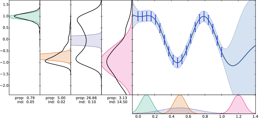
Our bound contains the trace of the conditional matrix (now in expectation), which we have studied in section 3.4. It also contains the usual KL divergence term from the prior. The final ‘regularization’ term (third line of (19)) has interesting regularization properties: it contains the variance of the GP function at each layer, under our approximation. To see this, if we are given the values of a GP function at , the mean of the prediction for the points at is given by . The sum of the variance of this vector is then , and the ‘regularization’ term is the variance of this under , in expectation under . The term summarizes how the values of the function will change as the input to the function changes: a measure of the local ‘wiggliness’ of the function under the variational input distribution.
We refer to these two regularization terms as the ‘compression term’ and the ‘propagation term’. In figure 2, we illustrate the forward passing of the Gaussian distributions (according to our likelihood computation) for different scenarios, and the incurred penalty terms. In summary, the regularization terms encourage approximations that can be well represented by the limited representative power of .
5 Experiments
We present three applications of the variationally compressed deep GP method. In each case, we used simple gradient based optimization to maximize the bound on the marginal likelihood with respect to the covariance function parameters, the inducing input positions in each layer, and the variational parameters of in each layer, . To maintain positive-definiteness of the covariance matrices, we employed a lower-triangular factorized representation, .
To exploit the factorised nature of the objective function, our python implementation uses MPI to parallelize computation across several cores of a desktop machine. Parallelism is across chunks of data, since equation LABEL:eq:deepBound can be written as a sum of data dependent terms. Parallelization to larger systems is straightforward, and the objective lends itself to stochastic optimization.
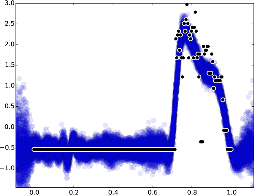
5.1 Step Function Data
In Rasmussen and Williams (2006), a simple example is presented which is challenging for standard GP regression: data representing a noisy step function as in Figure 3. The GP with exponentiated quadratic covariance is unable to satisfactorily fit to the data, as the top plot in Figure 3 shows. Rasmussen and Williams (2006) propose using a neural-network based covariance function, which is able to model the data somewhat better. Calandra et al. (2014) propose a two layer model where the data are transformed by some deterministic function before being passed into a GP, which appears to perform somewhat better, though this is arguably still a kernel selection problem, with parameters of the deterministic function being incorporated into the kernel.
The idea of deep networks is to avoid this kind of kernel selection, using layers of representation to infer features from the data. Can deep GPs do away with the problem of having to select a kernel in a Bayesian fashion? Figure 3 suggests that this might be the case. Moving down the panels of the Figure, the depth of the model is increased from 1 (a GP model) to 3. The GP model is unable to cope with the non-smoothness of the function, provides an ‘overshot’ mean function and extrapolates poorly. The two layer deep GP has more capability to fit the sharp change in the function though it still overshoots a little, and the three layer deep model performs well, with a sharp mean function at the step. Extrapolation from the data has interesting behaviour, we note that despite the posterior appearing bimodal, any sample drawn from the posterior will be a continuous function, which will switch between the two modes with a lengthscale of around 0.2.
5.2 Robot Wireless Data
Our second data set consists of a robotics localization problem (Ferris et al., 2007). We are presented with the signal strengths of thirty wireless access points located around a building, as detected by a robot which is tracing a path through the corridors. The wireless signal strengths fluctuate as a function of time as the robot moves nearer of further from each access point. The underlying structure of the signals must surely represent the position of the robot in the building.
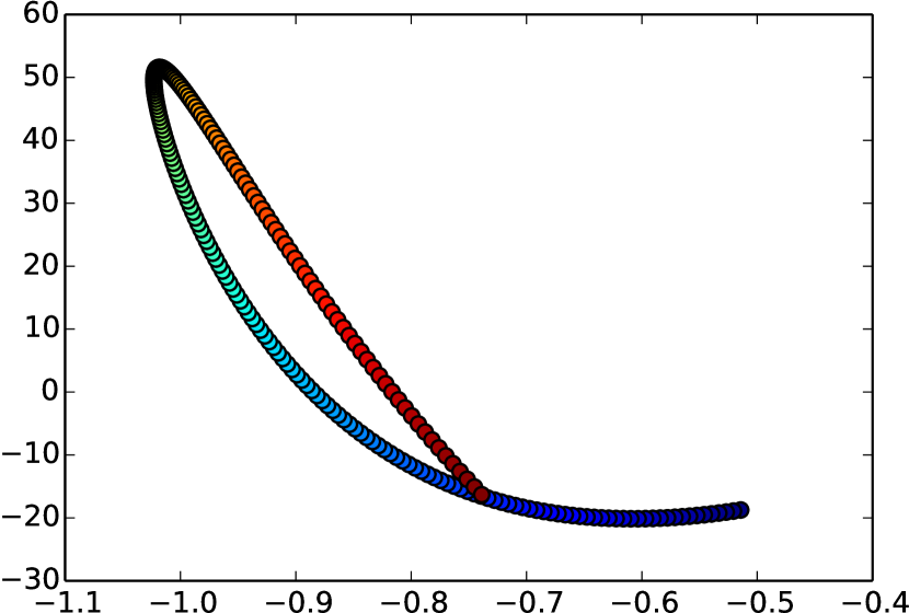
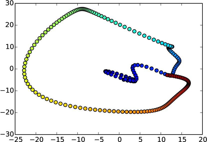
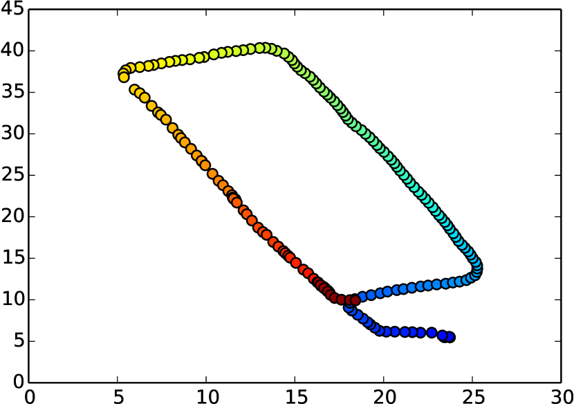
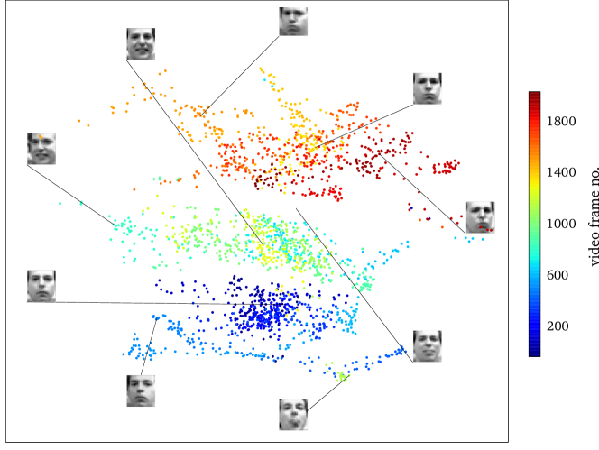
We build a 3 layer deep GP, in which the input layer was time, through two hidden layers with 3 dimensions each, and finally mapping to the 30 dimensional signal strengths. After optimization of the marginal-likelihood bound using L-BFGS-B (Zhu et al., 1997), the learned structure of the model is as in Figure 4.
Figure 4 (c) shows the true path of the robots, which completes a rectangular loop around the building, with a ’tail’ of data at the start. In the fist hidden layer (figure 4(a)), the models learns the topology of the structure: a loop closes at the correct point. In the subsequent layer, the representation contains ‘corners’, representing structure in the data where correlations in the signal strength must vary rapidly or slowly. This hierarchically structured learning of features is a key feature of the deep GP model which is not possible using a standard GP.
The final frame of figure 4 shows on of the thirty signals used. Two interesting features are prominent: the deep GP is insensitive to outliers (some occur at around ), and the deep GP predicts structure where none is present (around ). Both of these effects are a result of the strong structural prior imposed by the deep GP model: output variables are expected to covary in a consistent way, and structure in some part of the data is imposed on other parts also.
In both these cases, the strong structural prior is reasonable. At around the WiFi drops out because the device only retains the largest signals it can measure. However, the true underlying signal is still likely to covary with the other measurements in a fashion as predicted by the model. The outlying data are also explained well by the deep GP.
The variational approximation to the posterior is unimodal, and the deep GP prior contains many possible modes which can be constructed by symmetrical and rotational arguments. Re-running the experiment shown in figure 4 will result in a different representation each time. Selection of the ‘best’ approximating posterior is possible by comparing the bounds on the marginal likelihood. We note that the majority of solutions found for this problems qualitatively represent that presented in figure 4. There would also be scope to combine the variational approximations through mixture distributions (Lawrence, 2000).
5.3 Autoencoders
Building auto-encoding deep GPs is straightforward: we simple use the same data as input and output to the model.
We build a two-layer deep GP, with the same data on the input and output. That is, a single hidden representation with an ‘encoding’ layer and a ‘decoding’ layer. Using the Frey faces dataset (Frey et al., 1998), which has 784 dimensions (pixels) and approximately 2,000 training points, we optimized the marginal likelihood bound using L-BFGS-B (Zhu et al., 1997).
6 Discussion
We have shown how variational compression bounds can be applied to inference in deep Gaussian process models. The resulting bounds are scalable due to their decompositional nature over the data points. In analysing the bound on the deep GP marginal likelihood, we have seen that the approximation appears as a neural network structure, but with Gaussian messages being fed forward. We have shown how natural penalty terms arise which decrease the bound when the propagation of the Gaussian messages performs poorly.
This work opens the possibility of application of Deep GPs to big datasets for the first time.
References
- Álvarez et al. (2010) M. A. Álvarez, D. Luengo, M. K. Titsias, and N. D. Lawrence. Efficient multioutput Gaussian processes through variational inducing kernels. In Teh and Titterington (2010), pages 25–32.
- Calandra et al. (2014) R. Calandra, J. Peters, C. E. Rasmussen, and M. P. Deisenroth. Manifold Gaussian processes for regression. Technical report, 2014.
- Csató and Opper (2002) L. Csató and M. Opper. Sparse on-line Gaussian processes. Neural Computation, 14(3):641–668, 2002.
- Damianou and Lawrence (2013) A. Damianou and N. D. Lawrence. Deep Gaussian processes. In C. Carvalho and P. Ravikumar, editors, Proceedings of the Sixteenth International Workshop on Artificial Intelligence and Statistics, volume 31, AZ, USA, 2013. JMLR W&CP 31.
- Damianou et al. (2011) A. Damianou, M. K. Titsias, and N. D. Lawrence. Variational Gaussian process dynamical systems. In P. Bartlett, F. Peirrera, C. Williams, and J. Lafferty, editors, Advances in Neural Information Processing Systems, volume 24, Cambridge, MA, 2011. MIT Press.
- Denil et al. (2013) M. Denil, B. Shakibi, L. Dinh, M. Ranzato, and N. D. Freitas. Advances in neural information processing systems. In C. J. C. Burges, L. Bottou, Z. Ghahramani, M. Welling, and K. Q. Weinberger, editors, Advances in Neural Information Processing Systems, volume 26, pages 2148–2156, Cambridge, MA, 2013.
- Duvenaud et al. (2014) D. Duvenaud, O. Rippel, R. Adams, and Z. Ghahramani. Avoiding pathologies in very deep networks. In S. Kaski and J. Corander, editors, Proceedings of the Seventeenth International Workshop on Artificial Intelligence and Statistics, volume 33, Iceland, 2014. JMLR W&CP 33.
- Ferris et al. (2007) B. D. Ferris, D. Fox, and N. D. Lawrence. WiFi-SLAM using Gaussian process latent variable models. In M. M. Veloso, editor, Proceedings of the 20th International Joint Conference on Artificial Intelligence (IJCAI 2007), pages 2480–2485, 2007.
- Frey et al. (1998) B. J. Frey, A. Colmenarez, and T. S. Huang. Mixtures of local linear subspaces for face recognition. In Computer Vision and Pattern Recognition, 1998. Proceedings. 1998 IEEE Computer Society Conference on, pages 32–37. IEEE, 1998.
- Gal et al. (2014) Y. Gal, M. van der Wilk, and C. E. Rasmussen. Distributed variational inference in sparse Gaussian process regression and latent variable models. In Z. Ghahramani, M. Welling, C. Cortes, N. D. Lawrence, and K. Q. Weinberger, editors, Advances in Neural Information Processing Systems, volume 27, Cambridge, MA, 2014.
- Hensman et al. (2013) J. Hensman, N. Fusi, and N. D. Lawrence. Gaussian processes for big data. In A. Nicholson and P. Smyth, editors, Uncertainty in Artificial Intelligence, volume 29. AUAI Press, 2013.
- Hoffman et al. (2012) M. Hoffman, D. M. Blei, C. Wang, and J. Paisley. Stochastic variational inference. Technical report, 2012.
- Hornik et al. (1989) K. Hornik, M. Stinchcombe, and H. White. Multilayer feedforward networks are universal approximators. Neural Networks, 2(5):359–366, 1989.
- Kingma and Welling (2013) D. P. Kingma and M. Welling. Auto-encoding variational Bayes. Technical report, 2013.
- Lawrence (2000) N. D. Lawrence. Variational Inference in Probabilistic Models. PhD thesis, Computer Laboratory, University of Cambridge, New Museums Site, Pembroke Street, Cambridge, CB2 3QG, U.K., 2000. Available from http://www.thelawrences.net/neil.
- Lawrence and Moore (2007) N. D. Lawrence and A. J. Moore. Hierarchical Gaussian process latent variable models. In Z. Ghahramani, editor, Proceedings of the International Conference in Machine Learning, volume 24, pages 481–488. Omnipress, 2007. ISBN 1-59593-793-3.
- Lázaro-Gredilla (2012) M. Lázaro-Gredilla. Bayesian warped Gaussian processes. In P. L. Bartlett, F. C. N. Pereira, C. J. C. Burges, L. Bottou, and K. Q. Weinberger, editors, Advances in Neural Information Processing Systems, volume 25, Cambridge, MA, 2012.
- MacKay (1998) D. J. C. MacKay. Introduction to Gaussian Processes. In C. M. Bishop, editor, Neural Networks and Machine Learning, volume 168 of Series F: Computer and Systems Sciences, pages 133–166. Springer-Verlag, Berlin, 1998.
- Neal (1996) R. M. Neal. Bayesian Learning for Neural Networks. Springer, 1996. Lecture Notes in Statistics 118.
- Quiñonero Candela and Rasmussen (2005) J. Quiñonero Candela and C. E. Rasmussen. A unifying view of sparse approximate Gaussian process regression. Journal of Machine Learning Research, 6:1939–1959, 2005.
- Rasmussen and Williams (2006) C. E. Rasmussen and C. K. I. Williams. Gaussian Processes for Machine Learning. MIT Press, Cambridge, MA, 2006. ISBN 0-262-18253-X.
- Rezende et al. (2014) D. J. Rezende, S. Mohamed, and D. Wierstra. Stochastic back-propagation and variational inference in deep latent Gaussian models. Technical report, 2014.
- Snelson and Ghahramani (2006) E. Snelson and Z. Ghahramani. Sparse Gaussian processes using pseudo-inputs. In Y. Weiss, B. Schölkopf, and J. C. Platt, editors, Advances in Neural Information Processing Systems, volume 18, Cambridge, MA, 2006. MIT Press.
- Srivastava et al. (2014) N. Srivastava, G. Hinton, A. Krizhevsky, I. Sutskever, and R. Salakhutdinov. Dropout: A simple way to prevent neural networks from overfitting. Journal of Machine Learning Research, 15:1929–1958, 2014. URL http://jmlr.org/papers/v15/srivastava14a.html.
- Teh and Titterington (2010) Y. W. Teh and D. M. Titterington, editors. Artificial Intelligence and Statistics, volume 9, Chia Laguna Resort, Sardinia, Italy, 13-16 May 2010. JMLR W&CP 9.
- Titsias (2009) M. K. Titsias. Variational learning of inducing variables in sparse Gaussian processes. In D. van Dyk and M. Welling, editors, Proceedings of the Twelfth International Workshop on Artificial Intelligence and Statistics, volume 5, pages 567–574, Clearwater Beach, FL, 16-18 April 2009. JMLR W&CP 5.
- Titsias and Lawrence (2010) M. K. Titsias and N. D. Lawrence. Bayesian Gaussian process latent variable model. In Teh and Titterington (2010), pages 844–851.
- Williams (1998) C. K. I. Williams. Computation with infinite neural networks. Neural Computation, 10(5):1203–1216, 1998.
- Wilson and Adams (2013) A. G. Wilson and R. P. Adams. Gaussian process kernels for pattern discovery and extrapolation. In S. Dasgupta and D. McAllester, editors, ICML, volume 28 of JMLR Proceedings, pages 1067–1075. JMLR.org, 2013.
- Zhu et al. (1997) C. Zhu, R. H. Byrd, and J. Nocedal. L-BFGS-B: Algorithm 778: L-BFGS-B, FORTRAN routines for large scale bound constrained optimization. ACM Transactions on Mathematical Software, 23(4):550–560, 1997.