Complementary action of chemical and electrical synapses to perception

Abstract

We study the dynamic range of a cellular automaton model for a neuronal network with electrical and chemical synapses. The neural network is separated into two layers, where one layer corresponds to inhibitory, and the other corresponds to excitatory neurons. We randomly distribute electrical synapses in the network, in order to analyse the effects on the dynamic range. We verify that electrical synapses have a complementary effect on the enhancement of the dynamic range. The enhancement depend on the proportion of electrical synapses, and also depend on the layer where they are distributed.

Keywords: dynamic range, cellular automaton, neuron

1 Introduction

The cerebral cortex contains neurons and their fibres [1]. These neurons are grouped together into functional or morphological units, called cortical areas [2], each of them playing a well-defined role in the processing of information in the brain [3]. Hence the theoretical understanding of the principles of organisation and functioning of the cerebral cortex can shed light on the knowledge of many distinct and important subjects in neuroscience [4]. One relevant subject is psychophysics, that analyses the perceptions due to external stimuli [5].

Studies about the relation between sensation and stimulus by measuring the quantity of both factors were realised by Weber and Fechner [6]. They proposed that the relation was logarithmic [7]. However, Stevens proposed a theory based on a power-law relation between stimulus and response, where the exponent depends on the type of stimulation [9].

The capacity of a biological system to discriminate the intensity of an external stimulus is characterized by the dynamic range (DR) [10]. DR is a range of intensities for which receptors can encode stimuli [9, 11, 8]. It is the logarithm of the difference between the smallest and the largest stimulus value for which the responses are not too weak to be distinguished or too close to saturation, respectively. The lower and upper bounds are arbitrarily chosen due to the fact that the scaling region is well fit by a power law. In other words, small changes are not affect our results. The visual and the auditory perception have high dynamic range. The human sense of sight can perceive changes in about ten decades of luminosity, and the hearing covers twelve decades in a range of intensities of sound pressures [7]. The DR of the human visual is important in the design of high dynamic range display devices [12]. Whereas the DR of the hearing is used for cochlear implant systems [13].

In this work we study the dynamic range of a cellular automaton with electrical and chemical synapses [14]. We consider that the chemical synapses can be excitatory or inhibitory, and a layered model [15], where one layer consists of excitatory neurons, and the other layer consists of inhibitory neurons. Network consisting of excitatory and inhibitory neurons was considered to describe the primary visual cortex [16]. Pei and collaborators [17] investigated the behaviour of excitatory-inhibitory excitable networks with an external stimuli. They suggested that the dynamic range may be enhanced if high inhibitory factors are cut out from the inhibitory layer. In our work, we consider a neural network in which neurons interact by chemical and electrical synapses in a excitatory-inhibitory layered model. Our main results are: the equation of the dynamic range for a random neural network with chemical and electrical synapses, and to show that electrical synapses in the excitatory layer have an influence on the dynamic range more significative than in the inhibitory layer, due to the fact that the electrical synapses in the excitatory layer are responsible for the complementary effect of dynamic range enhancement.

This paper is organised as follows: in Section 2 we introduce the cellular automaton rule, and the random network. Section 3 shows our analytical and numerical results obtained for the dynamic range. The last section presents the conclusions.

2 Neuronal network model of spiking neurons

We consider a cellular automaton model in that a node can spike, $x_{i}=1$, when stimulated in its resting state, $x_{i}=0$ ($i=1,...,N$). When a spike occurs there is a refractory period until the node returns to its resting state, $x_{i}=2,...,\mu-1$. During the refractory period no spikes occur. There are excitatory and inhibitory connections linking nodes unidirectionally. The pre-synaptic node whose out chemical synapses is excitatory (inhibitory) is called an excitatory (inhibitory) node. Excitatory nodes increase the probability of excitation of their connected nodes, while inhibitory nodes decrease the probability. The network presents also electrical connections, that are bidirectional links. They increase the probability of excitation between the connected nodes.

The dynamics of the cellular automaton is given by:

1. if $x_{i}(t)=0$, then

   • a node can be inhibited by an excited inhibitory node $j$ ($x_{j}(t)=1$) with probability $B_{ij}$, remaining equal to zero in the next time step;

   • a node can be excited by an excited excitatory node $j^{\prime}$ ($x_{j^{\prime}}(t)=1$) with probability $B_{ij^{\prime}}$;

   • a node with electrical connection can be excited by an excited node $j^{\prime\prime}$ with probability $A_{ij^{\prime\prime}}$.

   • a node can be excited by an external stimulus with probability $r$.

2. if $x_{i}\neq 0$, then $x_{i}(t+1)=x_{i}(t)+1$ (mod $\mu$), where $x_{i}(t)\in\{0,1,...,\mu-1\}$ is the state of the $i$th node at time $t$. In other words, the node spikes ($x_{i}=1$) and after that remains insensitive during $\mu-2$ time steps.

The weighted adjacency matrices $A_{ij}$ and $B_{ij}$ describe the strength of interactions between the nodes. The matrix $A_{ij}$ contains information about the electrical connections, and the matrix $B_{ij}$ about the excitatory and inhibitory connections. The connection architecture is described by a random graph, in that the connections are randomly chosen [18]. We separete the neurons by layers. Figure 1 shows the scheme of the E-I layered network, where the E layer contains $N_{e}$ excitatory nodes, and the I layer contains $N_{i}$ inhibitory nodes. Then, the layered network has a total of $N_{e}+N_{i}=N$ nodes. The excitatory connections (blue circles) go from excitatory nodes to other nodes, the inhibitory connections (red squares) go from inhibitory nodes to other nodes, and the electrical connections are bidirectional (black saw lines).

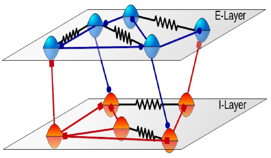
Figure 1: Scheme of the E-I layered network with one excitatory layer (E-layer), and one inhibitory layer (I-layer). The lines with blue filled circles represent the excitatory connections, the lines with red filled squares represent the inhibitory connections, and the other links represented by black saw line are the electrical connections.

The neuron responses are obtained through the density of spiking neuron

$$p(t)=\frac{1}{N}\sum_{i=1}^{N}\delta(x_{i}(t),1),$$ (1)

where $\delta(a,b)$ is the Kronecker delta. With the density we calculate the average firing rate

$$F=\overline{p(t)}=\frac{1}{T}\sum_{t=1}^{T}p(t),$$ (2)

$T$ is the time window chosen for the average.

The update rules for neurons in E and I layer are the same. In order to estimate analytically the average firing rate, we calculate the mean-field map for $p(t)$ at a long time

$$p(t+1) = [1-(\mu-1)p(t)](1-S_{\rm ch}p(t))^{f_{i}K_{\rm ch}}$$

$$\times \{r+(1-r)[1-(1-S_{\rm ch}p(t))^{f_{e}K_{\rm ch}}(1-S_{\rm el}p(t))^{K_{\rm el}}]\},$$

in which $S_{\rm ch}$ is the strength of excitatory and inhibitory interactions, $S_{\rm el}$ is the strength of electrical interactions, $f_{e}=N_{e}/N$ and $f_{i}=N_{i}/N$ are the fraction of excitatory and inhibitory nodes, respectively. The average degree of chemical connections is denoted by $K_{\rm ch}$, and $K_{\rm el}$ denotes the average degree of electrical connections. The average degree is calculated by assuming randomly chosen pairs of nodes.

To obtain an approximate analytical value for the firing rate ($F$) for the case of small density of spiking neuron ($p(t)$), and without an external perturbation ($r=0$), we expand Eq. (2) around $p(t)=0$, and find

$$p^{*}\approx\frac{\varepsilon+\sigma f_{e}-1}{(\mu-1)(\varepsilon+\sigma f_{e})+\sigma(\varepsilon+\sigma f_{e}f_{i})},$$ (4)

in a mean-field approximation [11] $\sigma=K_{\rm ch}S_{\rm ch}$ is the average chemical branching ratio of nodes in the E-layer, and $\varepsilon=K_{\rm el}S_{\rm el}$ is the average electrical branching ratio of nodes, representing the overall strength of chemical and electrical interaction in the network. We can write $p^{*}=p(t+1)=p(t)$ in the stationary state, and as a result for large time we have $F\approx p^{*}$. Figure 2 exhibits the firing rate varying $\sigma$ for different values of $\varepsilon$. The symbols correspond to simulation according to celular automaton rules, and the lines correspond to the theoretical values from Eq. (4).

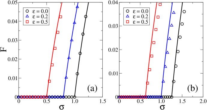
Figure 2: (Colour online) Firing rate versus branching ratio $\sigma$ for $N=10^{5}$, $K_{\rm ch}=10$, $S_{\rm el}=1$, $\mu=5$, $r=0$, (a) $f_{e}=1$, and (b) $f_{e}=0.8$. The symbols correspond to simulation results, and the lines are the theoretical values according to Eq. 4.

There is a critical value of the average branching ratio $\sigma_{c}$ in that the firing rate increases from zero. In other words, $\lim_{r\rightarrow 0}F=0$ if $\sigma<\sigma_{c}$, and $\lim_{r\rightarrow 0}F>0$ if $\sigma>\sigma_{c}$. We can see through Figures 2(a) and (b) that $\sigma_{c}$ depends on $f_{e}$ and $\varepsilon$. Equation (4) allows us to obtain the dependence, given by $\sigma_{c}=(1-\varepsilon)/f_{e}$, by assuming that $p$ is null. In Figure 3 we compare the simulation result (symbols) with the equation for $\sigma_{c}$ (lines). It is possible to see a good agreement. This shows that chemical and electrical connections complement themselves for obtaining the critical point $\sigma_{c}$. The larger (smaller) the electrical branching rate in the network, the smaller (larger) the chemical branching rate must be.

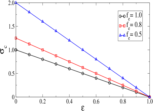
Figure 3: (Colour online) $\sigma_{c}$ versus $\varepsilon$ for $f_{e}=0.5$ (blue triangles), $f_{e}=0.8$ (red squares), and $f_{e}=1.0$ (black circles). The lines are from the analytical expression $\sigma_{c}=(1-\varepsilon)/f_{e}$.

3 Dynamic Range

The ratio between the largest and smallest possible values of a changeable quantity is called dynamic range. The standard definition of the dynamic range is [19]

$$\Delta=10\log_{10}\frac{r_{\rm high}}{r_{\rm low}},$$ (5)

where $r_{\rm high}$ and $r_{\rm low}$ are the average input rates for $F_{\rm high}$ and $F_{\rm low}$, respectively (Fig. 4). The high firing rate is obtained from $F_{\rm high}=F_{0}+0.95(F_{\rm max}-F_{0})$, and the low firing rate is from $F_{\rm low}=F_{0}+0.05(F_{\rm max}-F_{0})$, where $F_{0}$ is the value for the minimum saturation, and $F_{\rm max}$ is the value for the maximum saturation. If the system has a refractory time $\mu$, the maximum firing rate $F_{\rm max}$ is equal to $1/\mu$.

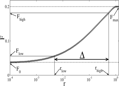
Figure 4: Average firing rate as a function of the average input rate.

Taking the limit of Eq. (2) as $p$ approaches zero

$$p\approx[1-(\mu-1)p]{\rm e}^{-f_{i}\sigma p}[r+(1-r)(1-{\rm e}^{-p(f_{e}\sigma+\varepsilon)})],$$ (6)

which allow us to obtain $r_{\rm low}$ by doing $r=r_{\rm low}$. Then, the dynamic range is given by

$$\Delta=-10\log_{10}\left[\frac{1-{\rm e}^{F_{\rm low}(f_{e}\sigma+\varepsilon)}}{r_{\rm high}}+\frac{F_{\rm low}{\rm e}^{F_{\rm low}(\sigma+\varepsilon)}}{r_{\rm high}-(\mu-1)F_{\rm low}r_{\rm high}}\right].$$ (7)

We have verified that $r_{\rm high}$ is approximately equal to $0.75$ for our simulation considering $N=10^{5}$, and $\mu=5$. By means of $F_{0}$ (Eq. 4) the firing rate $F_{\rm low}$ can be calculated through relation $F_{\rm low}=F_{0}+0.05(F_{\rm max}-F_{0})$.

In Figure 5 we compare the dynamic range calculated using simulation (a) and from Eq. (7) (b). We can see that the dynamic range is maximum for $\sigma_{c}$, which is obtained by assuming that $r=0$. In the subcritical region for $\sigma f_{e}+\varepsilon<1$ it is possible to observe that weak stimuli are amplified and the sensitivity is enlarged, as a result of the activity propagation among neighbours. Therefore, the dynamic range increases with $\sigma$ and $\varepsilon$. In the supercritical region for $\sigma f_{e}+\varepsilon>1$ the dynamic range decreases due to the fact that the average firing rate is positive, and masks the effect of weak stimuli. The theoretical result shows a good agreement with the simulation, except for the supercritical region. This occurs due to the fact that the values of $p(t)$ are not around zero in the supercritical region, and we have considered $p(t)$ around zero to obtain analytical results.

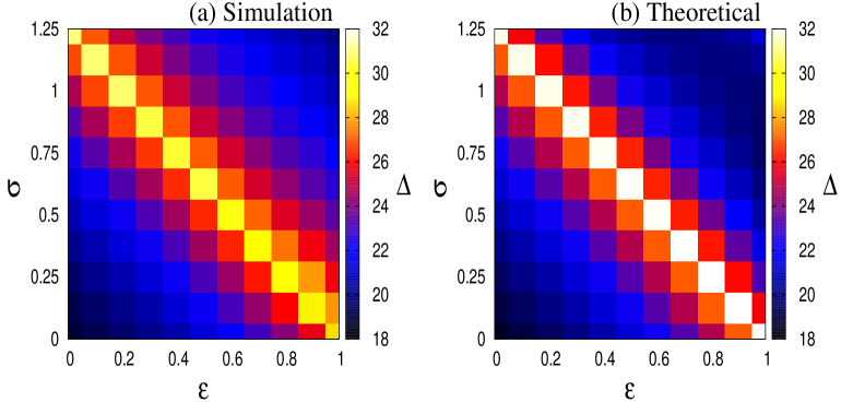
Figure 5: (Colour online) Dynamic range as a function of $\sigma$ and $\varepsilon$ for $N=10^{5}$, $K_{\rm ch}=10$, $S_{\rm el}=1$, $f_{e}=0.8$, and $\mu=5$. The simulation is showed in (a), and the result according to Eq. (7) is showed in (b).

3.1 Influence of electrical synapses

Pei and collaborators [17] investigated a excitatory-inhibitory excitable cellular automaton considering undirected random links. They verified that the dynamic range can be enhanced if the nodes with high inhibitory factors in the inhibitory layer are cut out. In this work, we are considering not only chemical synapses (directed links), but also electrical synapses (undirected links). Our interest is to understand the role of the electrical synapse in the dynamic range. For that goal Figure 5 shows the dynamic range for a network that has electrical synapses randomly distributed in all the network. We make further analysis considering the effect of electrical synapses on the dynamic range in two cases: (i) randomly distributed in the excitatory layer, and (ii) randomly distributed in the inhibitory layer.

Figure 6(a) shows the dynamic range for a network where electrical synapses are distributed in the excitatory layer. We can see that the behaviour of the dynamic range is similar to the one reported in Figure 5. The maximum dynamic range follows the equation for $\sigma_{c}$, namely the dynamic range can be enhanced increasing the amount of electrical synapses with the decrease of chemical synapses in the excitatory layer. However, when the electrical synapses are randomly distributed in the inhibitory layer, we do not observe a similar behaviour for the maximum dynamic range. In this case the dynamic range is affected by electrical synapses, but it is mainly enhanced by chemical synapses.

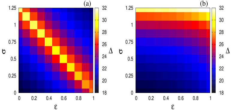
Figure 6: (Colour online) Dynamic range as a function of $\sigma$ and $\varepsilon$ for $N=10^{5}$, $K_{\rm ch}=10$, $S_{\rm el}=1$, $f_{e}=0.8$, and $\mu=5$. We consider randomly distributed electrical synapses in (a) excitatory layer, and (b) inhibitory layer.

4 Conclusions

We have modelled a neuronal network using cellular automaton which models the behaviour of a neural network where neurons interact by electrical and chemical synapses. The chemical synapses are separated into two layers, where one layer corresponds to excitatory, and the other corresponds to inhibitory.

Our aim has been to determine the dynamic range as a function of the types os synapses. Reference [17] shows theoretical analysis and simulations considering undirected connections. In this work, we have considered undirected electrical and directed chemical connections. Electrical and chemical synapses are relevant in cells found in the retina [20, 21], and cells in olfactory bulb [22].

We have obtained theoretical results for the average firing rate, and for the critical value of the average branching ratio that exits the network, allowing it to fire and consequently allowing information to be transmitted. From the equation of the average firing rate we obtained an equation for the dynamic range. This equation shows that the dynamic range is maximum for the critical average branching ratio. The equation presents a remarkable agreement with our simulations, mainly around the critical average branching rate. We verified an increase of the dynamic range in the subcritical region, and a decrease in the supercritical region. As a result, we verified that the enhacement of the dynamic range depends on the parameters $\varepsilon$ and $\sigma$ that are associated with the electrical and chemical synapses. Moreover, our results show that electrical synapses in the excitatory layer have an influence on the dynamic range more significative than when electrical synapses are placed in the inhibitory layer. The complementary effect occurs due to electrical synapses in the excitatory layer.

Reference

References

- [1] Kandel E R, Schwartz J H and Jessell T M 2000 Principles of Neural Science 4th edn (McGraw-Hill)
- [2] Rakic P 1988 Specification of cerebral cortical areas Science 241 170-176
- [3] Van Essen D C, Anderson C H and Felleman D J 1992 Information processing in the primate visual system: an integrated systems perspective Sci. 255 419-423
- [4] Buzsaki G 2006 Rhythms of the Brain (Oxford University Press)
- [5] Chescheider G A 2013 Psychophysics: The Fundamentals 3th edn (Psychology Press)
- [6] Murray D J 1993 A perspective for viewing the history of psychophysics Behav. Brain Sci. 16 115-186
- [7] Chialvo D R 2006 Are our senses critical Nat. Phys. 2 301-302
- [8] Batista C A S, Viana R L, Lopes S R and Batista A M 2014 Dynamic range in small-world networks of Hodgkin-Huxley neurons with chemical synapses Physica A 410 628-640
- [9] Stevens S S 2008 Psychophysics: Introduction to Its Perceptual Neural and Social Prospects (New Jersey: Transaction Publisher)
- [10] Gollo L L, Kinouchi O and Copelli M 2009 Active dendrites enhance neuronal dynamic range PLoS Comput. Biol. 5 e1000402
- [11] Kinouchi O and Copelli M 2006 Optimal dynamical range of excitable networks at criticality Nat. Phys. 2 348-351
- [12] Reinhard E, Ward G, Pattanaik S, Debevec P, Heidrich W and Myszkowski K 2010 High Dynamic Range Imaging: Acquisition, Display and Image-Based Lighting 2nd edn (Morgan Kaufmann Publishers)
- [13] Spahr A J, Dorman M F and Loiselle L H 2007 Performance of patients using different cochlear implant systems: effects of input dynamic range Ear Hear. 28 2 260-275
- [14] Viana R L, Borges F S, Iarosz K C, Batista A M, Lopes S R and Caldas I L 2014 Dynamic range in a neuron network with electrical and chemical synapses Commun. Nonlinear Sci. Numer. Simul. 19 164-172
- [15] Kurant M and Thiran P 2006 Layered complex networks Phys. Rev. Lett. 96 138701
- [16] Adini Y, Sagi D and Tsodyks 1997 Excitatory-inhibitory network in the visual cortex: Psychophysical evidence Proc. Natl. Acad. Sci. USA 94 10426
- [17] Pei S, Tang S, Yan S, Jiang S, Zhang X and Zheng Z 2012 How to enhance the dynamic range of excitatory-inhibitory excitable networks Phys. Rev. E 86 021909
- [18] Erdös P and Rényi 1959 On Random Graphs Publ. Math. 6 290-297
- [19] Firestein S, Picco C and Menini A 1993 The relation between stimulus and response in olfactory receptor cells of the tiger salamander J. Physiol. 468 1-10
- [20] Hidaka S, Akahori Y and Kurosawa Y 2005 Cellular/molecular dendrodendritic electrical synapses between mammalian retinal ganglion cells J. Neurosci. 24 10553-10567
- [21] Publio R, Ceballos C C and Roque A C 2012 Dynamic range of vertebrate retina ganglion cells: importance of active dendrites and coupling by electrical synapses PLoS ONE 7 e48517
- [22] Kosaka T, Deans M R, Paul D L and Kosaka K 2005 Neuronal gap junctions in the mouse main olfactory bulb: morphological analyses on transgenic mice Neurosci. 134 757-769