Highly comparative fetal heart rate analysis
Abstract
A database of fetal heart rate (FHR) time series measured from 7 221 patients during labor is analyzed with the aim of learning the types of features of these recordings that are informative of low cord pH. Our ‘highly comparative’ analysis involves extracting over 9 000 time-series analysis features from each FHR time series, including measures of autocorrelation, entropy, distribution, and various model fits. This diverse collection of features was developed in previous work [1], and is publicly available. We describe five features that most accurately classify a balanced training set of 59 ‘low pH’ and 59 ‘normal pH’ FHR recordings. We then describe five of the features with the strongest linear correlation to cord pH across the full dataset of FHR time series. The features identified in this work may be used as part of a system for guiding intervention during labor in future. This work successfully demonstrates the utility of comparing across a large, interdisciplinary literature on time-series analysis to automatically contribute new scientific results for specific biomedical signal processing challenges.
1 Introduction
During birth, a baby’s oxygen supply can be compromised and cause birth asphyxia (suffocation). Birth asphyxia can lead to seizures, permanent brain damage, and the death of the newborn. Intervention in the form of a Caesarean section, or the use of forceps or ventouse (vacuum), is required to prevent this chain of events, but such interventions can themselves cause complications and would preferably be avoided. Currently, the decision to intervene is made on the basis of an electronic recording of the baby’s heart rate during labor, a cardiotocogram (CTG). The mechanisms underlying this recording are complex and its analysis by eye is highly unreliable, whereby different experts can make conflicting decisions on the basis of the same CTG trace [2]. This subjectivity in decision-making can also lead to litigation when an ‘incorrect’ decision results in a complication. These factors have led to a push for research into an objective, computerized system for analyzing CTG recordings to assist the decision-making process [2]. Previous reports on this area have been plagued by very small datasets (typically containing less than 500 time series) [3, 4, 5]; it is difficult to reach reliable conclusions using such datasets for which so few compromised cases are available. The present work is distinguished both by the large size of the dataset: 7 221 FHR time series, and the scale of the analysis: over 9 000 time-series analysis features are compared.
Our primary aim in this paper is to contribute to a system being developed for intrapartum CTG analysis, OxSys [6], by providing a set of useful features derived from FHR time series. Rather than devising new types of features or manually comparing a small number of hand-picked candidates, we take the somewhat unusual approach in this work of comparing simultaneously the performance of thousands of features developed across the scientific time-series analysis literature. Using this highly comparative approach, those features that are the most successful are retrieved and subsequently analyzed and interpreted.
2 Data and Methods
2.1 Data
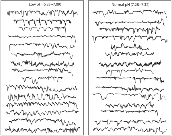
The initial dataset analyzed in this paper contains 7 568 FHR time series sampled at 4 Hz and recorded in the last 30 min before delivery. The data met a set of quality-based criteria from an initial set of 107 614 deliveries in John Radcliffe hospital, Oxford, UK between 20 April 1993 and 28 February 2008 [6], and were preprocessed to remove various known artifacts [7]. The data were processed further in this work: by linearly interpolating short durations of missing values, trimming longer durations of missing values, and removing time series with a large proportion of missing values, resulting in a dataset containing 7 221 FHR recordings. The data were partitioned into balanced training and test sets according to a previous study [6]. Within each set, each FHR recording is classified according to the cord pH of the corresponding baby, as either low pH () or normal pH (). The training set contains 59 time series of each class, and the the test set contains 117 time series of each class. Examples of both classes of time series in the training dataset are shown in Fig. 1.

2.2 Highly comparative analysis
Our highly comparative time-series analysis method is outlined in this section, and is described in detail elsewhere [1]. The method relies on a collection of 9 613 algorithms for extracting features from time series. These algorithms span a large variety of time-series properties, summarizing their autocorrelation, stationarity, summaries of their power spectra, wavelet decompositions, their distribution of values, fits to various time-series models (e.g., autoregressive, Gaussian Process, and Hidden Markov models), measures from the physical nonlinear time-series analysis literature (e.g., correlation dimension estimates, nonlinear prediction errors, fractal scaling properties), information theoretic quantities (e.g., permutation entropy, Sample Entropy, Lempel-Ziv Complexity), and others [1]. Each of these myriad methods is encoded in the same way: as an algorithm that maps an input time series to a single real number. Code for all time-series analysis methods used can be downloaded and explored at www.comp-engine.org/timeseries.
To compare their performance, all of these features were evaluated on all FHR time series in the dataset. Some algorithms could not be applied appropriately to some time series, e.g., fitting a positive-only distribution to time series that are not positive-only. In cases such as these, algorithms returned a special value: an infinity or a NaN. Features for which this occurred at least once across the dataset were removed from our analysis, and in this way, the initial set of 9 613 features was reduced to approximately 7 600 features.
2.3 Classification and Clustering
Classification rates quoted throughout this paper were obtained from a simple linear discriminant classifier, implemented using the classify function from Matlab’s Statistics Toolbox222We used Matlab 2011a. Matlab is a product of The MathWorks, Natick, MA., which provides a highly intuitive and interpretable result: a linear partition of the feature space [8]. For the single features focused on in this paper, linear classification boundaries are simply thresholds on the value of each feature.
Clustering is used to automatically reduce sets of features to smaller, representative subsets in this work. We used average linkage clustering, as implemented using the linkage function from Matlab’s Statistics Toolbox.
3 Results
3.1 Classification
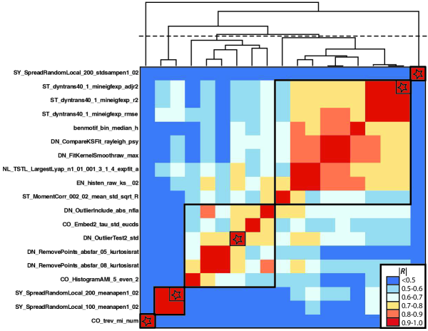
First we analyze the balanced training and test sets described above, with the aim of distinguishing FHR time series measured from fetuses with low cord pH at birth. We calculated the (in-sample) linear misclassification rates for each of 7 586 features (those with no special-valued outputs) on the training set. We then selected the nineteen most successful features: those with a false discovery rate [8] less than 0.001 (cf. [1]), corresponding to a linear misclassification rate under 30%. Since some of these nineteen features are highly correlated to one another across the dataset, we proceeded to construct a smaller set of features that minimizes this redundancy. Linear correlation coefficients calculated between all pairs of these nineteen features across the FHR dataset are shown in Fig. 2. A dendrogram relating the features was constructed using average linkage clustering and is shown above the pairwise correlation matrix in Fig. 2. By thresholding the dendrogram, the features were clustered into five groups. Features within each cluster have high linear correlations to one another and can be well-summarized by a single representative member. These representative features were chosen as those with the lowest misclassification rate in each cluster, and are labeled using stars in Fig. 2. In this way, a more manageable set of five relatively independent features was identified that effectively summarizes the most successful time-series analysis algorithms for distinguishing babies with low cord pH from FHR time series recorded during labor.

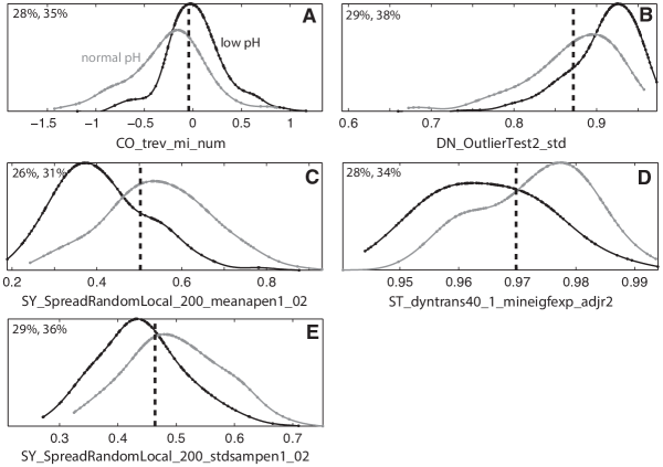
We now describe these five features, and investigate their performance on the test dataset. There is insufficient space to describe each feature in detail, but brief summaries are as follows: (i) CO_trev_mi_num is a quantity related to the time-reversal asymmetry of a time series, (ii) DN_OutlierTest2_std returns the ratio of standard deviations before and after removing 2% of the highest and lowest values of a time series, (iii) SY_SpreadRandomLocal_200_meanapen1_02 averages local Approximate Entropy [9], ApEn(1,0.2), estimates, (iv) ST_dyntrans40_1_mineigfexp_adjr2 calculates 1-step transition matrices for different alphabet sizes and fits a decaying exponential to the minimum eigenvalues of these transition matrices, and (v) SY_SpreadRandomLocal_200_stdsampen1_02 measures the variation in local Sample Entropy [10], SampEn(1,0.2), estimates from the time series. Distributions of the outputs of each of these features on the test data are shown in Fig. 3. These distributions provide an interpretable difference in the properties of the two groups of FHR time series: e.g., as shown in Fig. 3B, we see that healthy FHR recordings (gray) typically have more extreme outliers (and hence lower values of DN_OutlierTest2_std) compared to the low pH group (black). As indicated in Fig. 3, using a simple threshold on the output of each feature, in-sample misclassification rates range from 26%–29%, and out-of-sample misclassification rates range from 31%–38%. We note that classifiers that combine multiple features for this dataset (constructed using greedy forward feature selection [1]) showed no improvement in out-of-sample performance over single-feature classifiers.

3.2 Regression onto arterial cord pH
We now investigate features with outputs that correlate linearly with the cord pH across the full dataset of 7 221 FHR time series. The magnitude of linear correlation coefficients, , were low, with , but significantly larger than would be expected by chance (i.e., when the output of features are shuffled at random, cf. multiple hypothesis testing [8, 1]). In an analogous method to that shown for the classification task above, clustering was used to construct a set of five features that are representative of those with the strongest linear correlation coefficients, , to cord pH. These five features are now described briefly, with correlation coefficients given in parentheses: (i) coeff_var_2 () returns the second order coefficient of variation: , where and are the standard deviation and mean of the time series, respectively, (ii) median_absolute_deviation () returns the median absolute deviation, , a measure of spread of the time series, , (iii) ST_dyntrans40_1_mineigfexp_adjr2 () is a quantity derived from transition matrices, as described for the classification task above, (iv) DN_SimpleFit_exp1_rmse_h30 () returns the goodness of an exponential fit to the distribution of time-series values, and (v) CO_Embed2_tau_arearat () returns the ratio of areas spanned by points in a two-dimensional time-delay embedding space for the time series [11]. Interpreting the sign of the correlation also allows us to interpret the results directly; for example, DN_SimpleFit_exp1_rmse_h30 has , revealing that FHR recordings associated with a higher cord pH have distributions that are typically closer to exponential than those with lower cord pH.
3.3 EveREst plots
The great majority of FHR recordings studied in this work correspond to healthy babies with normal cord pH. For example, consider the following three groups: (i) low pH, defined as patients with an arterial cord pH , contains 302 patients, (ii) compromised, defined as patients with a reported severe, moderate, or mild reported compromise [6], contains 795 patients, and (iii) low pH and compromised, defined as patients that fulfill both of the above criteria, contains just 110 patients. These problematic cases may be preventable and are the most interesting to clinicians who must decide whether an intervention is appropriate in real time during labor. Distinguishing such small numbers of problematic scenarios from a large total cohort of 7 221 patients is difficult. One way of proceeding, which we follow here, is to divide the total cohort into equally-populated groups and compare the proportion of compromised cases in each group. A graphical representation of this approach has been termed an Event Rate Estimate (EveREst) plot [6].

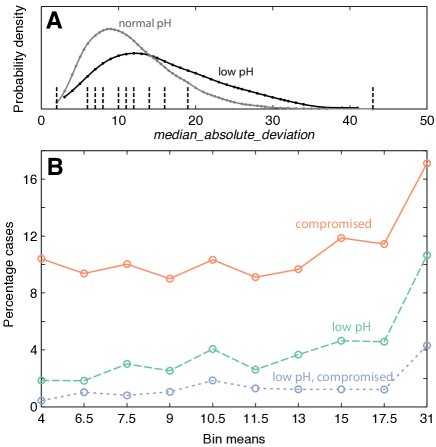
By ordering all FHR time series according to the value of a given feature, we constructed EveREst plots using for the successful features selected above. An example is shown in Fig. 4 for the median_absolute_deviation measure of spread, , which was selected from the regression task described above. Compared to the distributions shown in Fig. 3 for a balanced dataset, the distribution in Fig. 4A requires a more subtle interpretation, as the low pH condition (plotted black) contains just 302 recordings, compared to the 6 919 recordings with normal pH (plotted gray). However, dividing the patients into equal groups, as in Fig. 4B, reveals the proportion of problematic patients in each equally-populated group, which can be used to determine thresholds by which the two groups could be separated. Note that other features selected in the classification and regression tasks above have qualitatively similar EveREst plots to that shown in Fig. 4B.
For this median_absolute_deviation feature, there is a relatively sharp rise in low pH and compromised cases in the final bin. Patients in this bin: with , therefore have an increased risk of both delivering a baby with compromise, and of delivering a baby with low cord pH. As with most real-world applications, predicting compromise or low cord pH from FHR recordings is an complex and subtle problem that depends on a large number of variables. Thus, although not clinically useful on its own, this simple median_absolute_deviation measure of spread is both informative and extremely easy to compute. As much as an eight-fold increase in risk is observed here (for the low pH and compromised group in the final bin), making this feature a good candidate for further investigation in future work.
4 Conclusions
Five representative features were selected from those that were most successful at classifying FHR time series, and another five were selected to represent those with the strongest linear correlations to arterial cord pH across a dataset of 7 221 FHR time series. One of these features occurs in both sets, and hence we have a resulting set of nine candidate features that will be investigated as part of the Oxford System for intrapartum CTG analysis: OxSys [6]. Combined with features from other CTG recordings and additional clinical data, future work will focus on using these features to build a commercial diagnostic system—an intrapartum analogue of the established Dawes-Redman system [12].
Using the example of FHR analysis, this paper demonstrates the broad applicability of our highly comparative time-series analysis methodology [1]. The empirical structure of the labeled data was used to select features automatically, from a diverse and interdisciplinary scientific literature on time-series analysis. Although our set of over 9 000 features is far from exhaustive, we have successfully identified some of the most promising features from what is a comprehensive collection, and shown how they can be interpreted in the context of this FHR analysis problem. Extensive further work will be required to interpret the new features clinically, to integrate them into OxSys, and to study their relationships with existing FHR features. These candidate features will ultimately become components of multivariate analyses including other FHR features: standard morphological features (e.g., baseline, deceleration, variability) and clinical information about labour (e.g., use of epidural, gestation age). Code for all time-series analysis methods used here can be explored and downloaded at www.comp-engine.org/timeseries.
References
- Fulcher et al. [2013] B. D. Fulcher, M. A. Little, and N. S. Jones. Highly comparative time-series analysis: the empirical structure of time series and their methods. J. Roy. Soc. Interface 10, 20130048 (2013).
- Westgate [2009] J. Westgate. Medical informatics in obstetrics and gynecology. Medical Info Science Reference., chapter x: Computerizing the Cardiotocogram (CTG), pp. 151–158. Medical Information Science Reference (2009).
- Pello et al. [1991] L. C. Pello, S. K. Rosevear, G. S. Dawes, M. Moulden, and C. W. G. Redman. Computerized fetal heart rate analysis in labor. Obstet. Gynecol. 78 (1991).
- Warrick et al. [2010] P. A. Warrick, E. F. Hamilton, D. Precup, and R. E. Kearney. Classification of normal and hypoxic fetuses from systems modeling of intrapartum cardiotocography. IEEE T. Bio.-Med. Eng. 57, 771 (2010).
- Chudáček et al. [2011] V. Chudáček, J. Spilka, P. Janků, et al. Automatic evaluation of intrapartum fetal heart rate recordings: a comprehensive analysis of useful features. Physiol. Meas. 32, 1347 (2011).
- Georgieva et al. [2011] A. Georgieva, S. Payne, M. Moulden, and C. W. G. Redman. Artificial neural networks applied to fetal monitoring in labour. Neural Comput. Appl. (2011). In press, doi: 10.1007/s00521-011-0743-y.
- Georgieva et al. [2010] A. E. Georgieva, S. J. Payne, M. Moulden, and C. W. G. Redman. Automated fetal heart rate analysis in labor: Decelerations and overshoots. AIP Conf. Proc. 1293, 255 (2010).
- Hastie et al. [2009] T. Hastie, R. Tibshirani, and J. Friedman. The Elements of Statistical Learning: Data Mining, Inference, and Prediction. Springer, 2nd edition (2009).
- Pincus et al. [1991] S. M. Pincus, I. M. Gladstone, and R. A. Ehrenkranz. A regularity statistic for medical data analysis. J. Clin. Monitor Comp. 7, 335 (1991).
- Richman and Moorman [2000] J. S. Richman and J. R. Moorman. Physiological time-series analysis using approximate entropy and sample entropy. Am. J. Physiol. Heart Circ. Physiol. 278, H2039 (2000).
- Kantz and Schreiber [2004] H. Kantz and T. Schreiber. Nonlinear Time Series Analysis. Cambridge University Press, Cambridge, 2nd edition (2004).
- Pardey et al. [2002] J. Pardey, M. Moulden, and C. W. G. Redman. A computer system for the numerical analysis of nonstress tests. Am. J. Obstet. Gynecol. 186, 1095 (2002).