Lotka Volterra with randomly fluctuating environments
or
"how switching between beneficial environments can make survival harder"

Abstract

We consider two dimensional Lotka-Volterra systems in a fluctuating environment. Relying on recent results on stochastic persistence and piecewise deterministic Markov processes, we show that random switching between two environments that are both favorable to the same species can lead to the extinction of this species or coexistence of the two competing species.

MSC:

60J99; 34A60

Keywords:

Population dynamics, Persistence, Piecewise deterministic processes, Competitive Exclusion, Markov processes

Contents

1. 1 Introduction
   1. 1.1 Model, notation and presentation of main results
2. 2 Invasion rates
   1. 2.1 Jointly favorable environments
3. 3 Extinction
   1. 3.1 Proofs of Theorems 3.1, 3.3 and 3.4
4. 4 Persistence
   1. 4.1 Proof of Theorem 4.1
   2. 4.2 The support of the invariant measure
5. 5 Illustrations
6. 6 Proofs of Propositions 2.1 and 2.3
   1. 6.1 Proof of Proposition 2.1
   2. 6.2 Proof of Proposition 2.3

1 Introduction

In ecology, the principle of competitive exclusion formulated by Gause [17] in 1932 and later popularized by Hardin [19], asserts that when two species compete with each other for the same resource, the "better" competitor will eventually exclude the other. While there are numerous evidences (based on laboratory experiences and natural observations) supporting this principle, the observed diversity of certain communities is in apparent contradiction with Gause’s law. A striking example is given by the phytoplankton which demonstrate that a number of competing species can coexist despite very limited resources. As a solution to this paradox, Hutchinson [24] suggested that sufficiently frequent variations of the environment can keep species abundances away from the equilibria predicted by competitive exclusion. Since then, the idea that temporal fluctuations of the environment can reverse the trend of competitive exclusion has been widely explored in the ecology literature (see e.g [12], [1] and [10] for an overview and much further references).

Our goal here is to investigate rigorously this phenomenon for a two-species Lotka-Volterra model of competition under the assumption that the environment (defined by the parameters of the model) fluctuates randomly between two environments that are both favorable to the same species. We will precisely describe -in terms of the parameters- the range of possible behaviors and explain why counterintuitive behaviors - including coexistence of the two species, or extinction of the species favored by the environments - can occur.

Throughout, we let ${\mathbb{R}}$ (respectively ${\mathbb{R}}_{+},{\mathbb{R}}_{+}^{*}$) denote the set of real (respectively non negative, positive) numbers.

An environment is a pair $\mathcal{E}=(A,B)$ defined by two matrices

$$A=\left(\begin{array}[]{cc}a&b\\ c&d\\ \end{array}\right),B=\left(\begin{array}[]{c}\alpha\\ \beta\\ \end{array}\right),$$ (1)

where $a,b,c,d,\alpha,\beta$ are positive numbers.

The two-species competitive Lotka-Volterra vector field associated to $\mathcal{E}$ is the map $F_{\mathcal{E}}:{\mathbb{R}}^{2}\mapsto{\mathbb{R}}^{2}$ defined by

$$F_{\mathcal{E}}(x,y)=\left\{\begin{array}[]{c}\alpha x(1-ax-by)\\ \beta y(1-cx-dy)\end{array}\right..$$ (2)

Vector field $F_{\cal E}$ induces a dynamical system on ${\mathbb{R}}_{+}^{2}$ given by the autonomous differential equation

$$(\dot{x},\dot{y})=F_{\mathcal{E}}(x,y).$$ (3)

Here $x$ and $y$ represent the abundances of two species (denoted the x-species and y-species for notational convenience) and (3) describes their interaction in environment ${\cal E}.$

Environment ${\cal E}$ is said to be favorable to species x if

$$a<c\mbox{ and }b<d.$$

In other words, the intraspecific competition within species x (measured by the parameter $a$) is smaller than the interspecific competition effect of species x on species y (measured by $c$) and the interspecific competition effect of species y on species x is smaller that the intraspecific competition within species $\textbf{y}.$

From now on, we let $\mathsf{Env}_{\textbf{x}}$ denote the set of environments favorable to species $\textbf{x}.$ The following result easily follows from an isocline analysis (see e.g  [23], Chapter 3.3). It can be viewed as a mathematical formulation of the competitive exclusion principle.

Proposition 1.1

Suppose $\mathcal{E}=(A,B)\in\mathsf{Env}_{\textbf{x}}.$ Then, for every $(x,y)\in{\mathbb{R}}_{+}^{*}\times{\mathbb{R}}_{+}$ the solution to (3) with initial condition $(x,y)$ converges to $\displaystyle{(\frac{1}{a},0)}$ as $t\rightarrow\infty.$

If one now wants to take into account temporal variations of the environment, the autonomous system (3) should be replaced by the non-autonomous one

$$(\dot{x},\dot{y})=F_{{\cal E}(t)}(x,y),$$ (4)

where, for each $t\geq 0,$ ${\cal E}(t)$ is the environment at time $t.$ The story began in the mid $1970^{\prime}s$ with the investigation of systems living in a periodic environment (typically justified by the seasonal or daily fluctuation of certain abiotic factors such as temperature or sunlight). In 1974, Koch [25], formalizing Hutchinson’s ideas, described a plausible mechanism - sustained by numerical simulations - explaining how two species which could not coexist in a constant environment can coexist when subjected to an additional periodic kill rate (like seasonal harvesting or seasonal reduction of the population). More precisely, this means that $F_{{\cal E}(t)}(x,y)$ writes

$$F_{{\cal E}(t)}(x,y)=F_{{\cal E}}(x,y)-(p(t)x,q(t)y)$$

where $\mathcal{E}\in\mathsf{Env}_{\textbf{x}}$ and $p(t),q(t)$ are periodic positive rates. In 1980, Cushing [13] proves rigourously that, under suitable conditions on $\mathcal{E},p$ and $q,$ such a system may have a locally attracting periodic orbit contained in the positive quadrant ${\mathbb{R}}_{+}^{*}\times{\mathbb{R}}_{+}^{*}$.

In the same time and independently, de Mottoni and Schiaffino [14] prove the remarkable result that, when $t\rightarrow\mathcal{E}(t)$ is $T$-periodic, every solution to (4) is asymptotic to a $T$-periodic orbit and construct an explicit example having a locally attracting positive periodic orbit, while the averaged system (the autonomous system (3) obtained from (4) by temporal averaging) is favorable to the x-species. Papers [13] and [14] are complementary. The first one relies on bifurcations theory. The second makes a crucial use of the monotonicity properties of the Poincar map ($x,y\mapsto(x(T),y(T)$) and has inspired a large amount of work on competitive dynamics (see e.g  the discussion and the references following Corollary 5.30 in [20]).

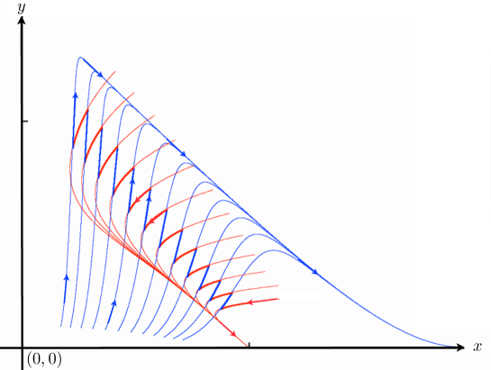
Completely different is the approach proposed by Lobry, Sciandra, and Nival in [27]. Based on classical ideas in system theory, this paper considers the question from the point of view of what is now called a switched system and focus on the situation where $t\rightarrow{\cal E}(t)$ is piecewise constant and assumes two possible values ${\cal E}_{0},{\cal E}_{1}\in\mathsf{Env}_{\textbf{x}}.$ For instance, Figure 3 pictures two phase portraits (respectively colored in red and blue) associated to the environments

$${\cal E}_{0}=\left(\left(\begin{array}[]{cc}1&1\\ 2&2\\ \end{array}\right),\left(\begin{array}[]{c}10\\ 1\\ \end{array}\right)\right)\mbox{ and }{\cal E}_{1}=\left(\left(\begin{array}[]{cc}0.5&0.5\\ 0.65&0.65\\ \end{array}\right),\left(\begin{array}[]{c}1\\ 10\\ \end{array}\right)\right)$$

both favorable to species $\textbf{x}.$ In accordance with Proposition 1.1 we see that all the red (respectively blue) trajectories converge to the $x$-axis while a switched trajectory like the one shown on the picture moves away from the $x$-axis toward the upper left direction. This was exploited in [27] to shed light on some paradoxical effect that had not been previously discussed in the literature: Even when ${\cal E}(t)\in\mathsf{Env}_{\textbf{x}}$ for all $t\geq 0$ (which is different from the assumption that the average vector field is induced by some ${\cal E}\in\mathsf{Env}_{\textbf{x}}$) not only coexistence of species but also extinction of species x can occur.

Figure 1: An example of switched trajectory.

In the present paper we will pursue this line of research and investigate thoroughly the behavior of the system obtained when the environment is no longer periodic but switches randomly between ${\cal E}_{0}$ and ${\cal E}_{1}$ at jump times of a continuous time Markov chain. Our motivation is twofold: First, realistic models of environment variability should undoubtedly incorporate stochastic fluctuations. Furthermore, the mathematical techniques involved for analyzing such a process are totally different from the deterministic ones mentioned above and will allow to fully characterize the long term behavior of the process in terms of quantities which can be explicitly computed.

1.1 Model, notation and presentation of main results

From now on we assume given two environments $\mathcal{E}_{0},\mathcal{E}_{1}\in\mathsf{Env}_{\textbf{x}}.$ For $i=0,1,$ environment $\mathcal{E}_{i}$ is defined by (1) with $(a_{i},b_{i},\ldots)$ instead of $(a,b,\ldots).$ We consider the process $\{(X_{t},Y_{t})\}$ defined by the differential equation

$$(\dot{X},\dot{Y})=F_{\mathcal{E}_{I_{t}}}(X,Y)$$ (5)

where $I_{t}\in\{0,1\}$ is a continuous time jump process with jump rates $\lambda_{0},\lambda_{1}>0.$ That is

$${\mathbb{P}}(I_{t+s}=1-i|I_{t}=i,{\cal F}_{t})=\lambda_{i}s+o(s)$$

where $\mathcal{F}_{t}$ is the sigma field generated by $\{I_{u},u\leq t\}.$

In other words, assuming that $I_{0}=i$ and $(X_{0},Y_{0})=(x,y),$ the process $\{(X_{t},Y_{t})\}$ follows the solution trajectory to $F_{\mathcal{E}_{i}}$ with initial condition $(x,y)$ for an exponentially distributed random time, with intensity $\lambda_{i}$. Then, $\{(X_{t},Y_{t})\}$ follows the the solution trajectory to $F_{\mathcal{E}_{1-i}}$ for another exponentially distributed random time, with intensity $\lambda_{1-i}$ and so on.

For $\eta>0$ small enough, the set

$$K_{\eta}=\{(x,y)\in{\mathbb{R}}_{+}^{2}\>:\eta\leq x+y\leq 1/\eta\}$$

is positively invariant under the dynamics induced by $F_{\mathcal{E}_{0}}$ and $F_{\mathcal{E}_{1}}.$ It then attracts every solution to (5) with initial condition $(x,y)\in{\mathbb{R}}_{+}^{2}\setminus\{0,0\}.$ Fix such $\eta>0$ and let

$$M=K_{\eta}\times\{0,1\}.$$

Set $Z_{t}=(X_{t},Y_{t},I_{t}).$ Since $Z_{t}$ eventually lies in $M$ (whenever $(X_{0},Y_{0})\neq(0,0)$) we may assume without loss of generality that $Z_{0}\in M$ and we see $M$ as the state space of the process $\{Z_{t}\}_{t\geq 0}.$

The extinction set of species y is the set

$$M_{0}^{\textbf{y}}=\{(x,y,i)\in M\>:y=0\}.$$

Extinction set of species $\textbf{x},$ denoted $M_{0}^{\textbf{x}}$, is defined similarly (with $x=0$ instead of $y=0$) and the extinction set is defined as

$$M_{0}=M_{0}^{\textbf{x}}\cup M_{0}^{\textbf{y}}.$$

The process $\{Z_{t}\}$ defines an homogeneous Markov process on $M$ leaving invariant the extinction sets $M_{0}^{\textbf{x}},M_{0}^{\textbf{y}}$ and the interior set $M\setminus M_{0}.$

It is easily seen that $\{Z_{t}\}$ restricted to one of the sets $M_{0}^{\textbf{y}}$ or $M_{0}^{\textbf{x}}$ is positively recurrent. In order to describe its behavior on $M\setminus M_{0}$ we introduce the invasion rates of species y and x as

$$\Lambda_{\textbf{y}}=\int\beta_{0}(1-c_{0}x)\mu(dx,0)+\int\beta_{1}(1-c_{1}x)\mu(dx,1),$$ (6)

and

$$\Lambda_{\textbf{x}}=\int\alpha_{0}(1-b_{0}y)\hat{\mu}(dy,0)+\int\alpha_{1}(1-b_{1}y)\hat{\mu}(dy,1).$$ (7)

where $\mu$ (respectively $\hat{\mu}$) denotes the invariant probability measure of $\{Z_{t}\}$ on $M_{0}^{\textbf{y}}$ (respectively $M_{0}^{\textbf{x}}$).

Note that the quantity $\beta_{i}(1-c_{i}x)$ is the growth rate of species y in environment $\mathcal{E}_{i}$ when its abundance is zero. Hence, $\Lambda_{\textbf{y}}$ measures the long term effect of species x on the growth rate of species y when this later has low density. When $\Lambda_{\textbf{y}}$ is positive (respectively negative) species y tends to increase (respectively decrease) from low density. Coexistence criteria based on the positivity of average growth rates go back to Turelli [33] and have been used for a variety of deterministic ([21], [16], [29]) and stochastic ([11], [10], [5] [15]) models. However, these criteria are seldom expressible in terms of the parameters of the model (average growth rates are hard to compute) and typically provide only local information on the behavior of the process near the boundary. Here surprisingly, $\Lambda_{\textbf{x}}$ and $\Lambda_{\textbf{y}}$ can be computed and their signs fully characterize the behavior of the process.

Our main results can be briefly summarized as follows.

(i)

The invariant measures $\mu,\hat{\mu}$ and the invasion rates $\Lambda_{\textbf{y}}$ and $\Lambda_{\textbf{x}}$ can be explicitly computed in terms of the parameters ${\cal E}_{i},\lambda_{i},i=0,1$ (see Section 2).

(ii)

For all $u,v\in\{+,-\}$ there are environments ${\cal E}_{0},{\cal E}_{1}\in\mathsf{Env}_{\textbf{x}}$ such that $Sign(\Lambda_{\textbf{x}})=u$ and $Sign(\Lambda_{\textbf{y}})=v.$ Thus, in view of assertion $(iii)$ below, the assumption that both environments are favorable to species x is not sufficient do determine the outcome of the competition.

(iii)

Let $(u,v)=(Sign(\Lambda_{\textbf{x}}),Sign(\Lambda_{\textbf{y}})).$ Assume $X_{0}>0$ and $Y_{0}>0.$ Then $(u,v)$ determines the long term behavior of $\{Z_{t}\}$ as follows.

(a)

$(u,v)=(+,-)\Rightarrow\mbox{ extinction of species {y}:}$

With probability one $Y_{t}\rightarrow 0$ and the empirical occupation measure of $\{Z_{t}\}$ converges to $\mu$ (see Theorem 3.1).

(b)

$(u,v)=(-,+)\Rightarrow\mbox{ extinction of species {x}:}$

With probability one $X_{t}\rightarrow 0$ and the empirical occupation measure of $\{Z_{t}\}$ converges to $\hat{\mu}$ (see Theorem 3.3).

(c)

$(u,v)=(-,-)\Rightarrow\mbox{ Extinction of one species:}$

With probability one either $X_{t}\rightarrow 0$ or $Y_{t}\rightarrow 0.$ The event $\{Y_{t}\rightarrow 0\}$ has positive probability. Furthermore, if the initial condition $X_{0}$ is sufficiently small or $(-,+)$ is feasible for ${\cal E}_{0},{\cal E}_{1},$ then the event $\{X_{t}\rightarrow 0\}$ has positive probability (see Theorem 3.4).

(d)

$(u,v)=(+,+)\Rightarrow\mbox{ persistence:}$

There exists a unique invariant (for $\{Z_{t}\}$) probability measure $\Pi$ on $M\setminus M_{0}$ which is absolutely continuous with respect to the Lebesgue measure $dxdy\otimes(\delta_{0}+\delta_{1});$ and the empirical occupation measure of $\{Z_{t}\}$ converges almost surely to $\Pi.$ Furthermore, for generic parameters, the law of the process converge exponentially fast to $\Pi$ in total variation. (see Theorem 4.1).

The density of $\Pi$ cannot be explicitly computed, still its tail behavior (Theorem 4.1, $(ii)$) and the topological properties of its support are well understood (see Theorem 4.5).

The proofs rely on recent results on stochastic persistence given in [4] built upon previous results obtained for deterministic systems in [21, 29, 16, 22] (see also [32] for a comprehensive introduction to the deterministic theory), stochastic differential equations with a small diffusion term in [5], stochastic differential equations and random difference equations in [31, 30]. We also make a crucial use of some recent results on piecewise deterministic Markov processes obtained in [2, 3] and [7].

The paper is organized as follows. In Section 2 we compute $\Lambda_{\textbf{x}}$ and $\Lambda_{\textbf{y}}$ and derive some of their main properties. Section 3 is devoted to the situation where one invasion rate is negative and contains the results corresponding to the cases $(iii),(a),(b),(c)$ above. Section 4 is devoted to the situation where both invasion rates are positive and contains the results corresponding to $(iii),(d)$. Section 5 presents some illustrations obtained by numerical simulation and Section 6 contains the proofs of some propositions stated in section 2.

2 Invasion rates

As previously explained, the signs of the invasion rates will prove to be crucial for characterizing the long term behavior of $\{Z_{t}\}.$ In this section we compute these rates and investigate some useful properties of the maps

$$(\lambda_{0},\lambda_{1})\mapsto\Lambda_{x}(\lambda_{0},\lambda_{1}),\Lambda_{y}(\lambda_{0},\lambda_{1})$$

and their zero sets.

Set $p_{i}=\frac{1}{a_{i}}$ and $\gamma_{i}=\frac{\lambda_{i}}{\alpha_{i}}.$ Here, for notational convenience, $[p_{0},p_{1}]$ (respectively $]p_{0},p_{1}[$) stands for the closed (respectively open) interval with boundary points $p_{0},p_{1}$ even when $p_{1}<p_{0},$ and $M_{0}^{\textbf{y}}$ is seen as a subset of ${\mathbb{R}}_{+}^{*}\times\{0,1\}.$

The following proposition characterizes the behavior of the process on the extinction set $M_{0}^{\textbf{y}}.$ The proof (given in Section 6) heavily relies on the fact that the process restricted to $M_{0}^{\textbf{y}}$, reduces to a one dimensional ODE with two possible regimes for which explicit computations are possible. It is similar to some result previously obtained in [8] for linear systems.

Proposition 2.1

The process $\{Z_{t}=(X_{t},Y_{t},I_{t})\}$ restricted to $M_{0}^{\textbf{y}}$ has a unique invariant probability measure $\mu$ satisfying:

(i)

If $p_{0}=p_{1}=p$

$$\mu=\delta_{p}\otimes\nu$$

where $\nu=\frac{\lambda_{0}}{\lambda_{1}+\lambda_{0}}\delta_{1}+\frac{\lambda_{1}}{\lambda_{1}+\lambda_{0}}\delta_{0}.$

(ii)

If $p_{0}\neq p_{1}$

$$\mu(dx,1)=h_{1}(x){\mathbf{1}}_{[p_{0},p_{1}]}(x)dx,$$

$$\mu(dx,0)=h_{0}(x){\mathbf{1}}_{[p_{0},p_{1}]}(x)dx$$

where

$$h_{1}(x)=C\frac{p_{1}|x-p_{1}|^{\gamma_{1}-1}|p_{0}-x|^{\gamma_{0}}}{\alpha_{1}x^{1+\gamma_{0}+\gamma_{1}}},$$

$$h_{0}(x)=C\frac{p_{0}|x-p_{1}|^{\gamma_{1}}|p_{0}-x|^{\gamma_{0}-1}}{\alpha_{0}x^{1+\gamma_{0}+\gamma_{1}}}$$

and $C$ (depending on $p_{1},p_{0},\gamma_{1},\gamma_{0}$) is defined by the normalization condition

$$\int_{]p_{0},p_{1}[}(h_{1}(x)+h_{0}(x))dx=1.$$

For all $x\in]p_{0},p_{1}[$ define

$$\theta(x)=\frac{|x-p_{0}|^{\gamma_{0}-1}|p_{1}-x|^{\gamma_{1}-1}}{x^{1+\gamma_{0}+\gamma_{1}}}$$ (8)

and

$$P(x)=[\frac{\beta_{1}}{\alpha_{1}}(1-c_{1}x)(1-a_{0}x)-\frac{\beta_{0}}{\alpha_{0}}(1-c_{0}x)(1-a_{1}x)]\frac{a_{1}-a_{0}}{|a_{1}-a_{0}|}.$$ (9)

Recall that the invasion rate of species y is defined (see equation (7)) as the growth rate of species y averaged over $\mu.$ It then follows from Proposition 2.1 that

Corollary 2.2

$$\Lambda_{\textbf{y}}=\left\{\begin{array}[]{ll}\frac{1}{\lambda_{0}+\lambda_{1}}(\lambda_{1}\beta_{0}(1-c_{0}p)+\lambda_{0}\beta_{1}(1-c_{1}p))&\hbox{if }p_{0}=p_{1}=p,\\ \displaystyle{p_{0}p_{1}C\int_{]p_{0},p_{1}[}P(x)\theta(x)dx}&\hbox{if }p_{0}\neq p_{1}\end{array}\right..$$ (10)

The expression for $\Lambda_{\textbf{x}}$ is similar. It suffices in equation (10) to permute $\alpha_{i}$ and $\beta_{i},$ and to replace $(a_{i},c_{i})$ by $(d_{i},b_{i})$ .

2.1 Jointly favorable environments

For all $0\leq s\leq 1,$ we let $\mathcal{E}_{s}=(A_{s},B_{s})$ be the environment defined by

$$sF_{\mathcal{E}_{1}}+(1-s)F_{\mathcal{E}_{0}}=F_{\mathcal{E}_{s}}$$ (11)

Then, with the notation of Section 1.1,

$$B_{s}=\left(\begin{array}[]{c}\alpha_{s}\\ \beta_{s}\\ \end{array}\right)=\left(\begin{array}[]{c}s\alpha_{1}+(1-s)\alpha_{0}\\ s\beta_{1}+(1-s)\beta_{0}\\ \end{array}\right)$$

and

$$A_{s}=\left(\begin{array}[]{ccc}a_{s}&b_{s}\\ \\ c_{s}&d_{s}\\ \end{array}\right)=\left(\begin{array}[]{ccc}\frac{s\alpha_{1}a_{1}+(1-s)\alpha_{0}a_{0}}{\alpha_{s}}&\frac{s\alpha_{1}b_{1}+(1-s)\alpha_{0}b_{0}}{\alpha_{s}}\\ \\ \frac{s\beta_{1}c_{1}+(1-s)\beta_{0}c_{0}}{\beta_{s}}&\frac{s\beta_{1}d_{1}+(1-s)\beta_{0}d_{0}}{\beta_{s}}\\ \end{array}\right).$$

Environment $\mathcal{E}_{s}$ can be understood as the environment whose dynamics (i.e the dynamics induced by $F_{\mathcal{E}_{s}}$) is the same as the one that would result from high frequency switching giving weight $s$ to $\mathcal{E}_{1}$ and weight $(1-s)$ to $\mathcal{E}_{0}.$

Set

$$I=\{0<s<1:\>a_{s}>c_{s}\}$$ (12)

and

$$J=\{0<s<1:\>b_{s}>d_{s}\}.$$ (13)

It is easily checked that $I$ (respectively $J$) is either empty or is an open interval which closure is contained in $]0,1[.$

To get a better understanding of what $I$ and $J$ represent, observe that

• If $s\in I^{c}\cap J^{c},$ then $\mathcal{E}_{s}$ is favorable to species $x;$

• If $s\in I\cap J,$ then $\mathcal{E}_{s}$ is favorable to species $y;$

• If $s\in I\cap J^{c},$ then $F_{\mathcal{E}_{s}}$ has a positive sink whose basin of attraction contains the positive quadrant (stable coexistence regime);

• If $s\in I^{c}\cap J,$ then $F_{\mathcal{E}_{s}}$ has a positive saddle whose stable manifold separates the basins of attractions of $(1/a_{s},0)$ and $(0,1/d_{s})$ (bi-stable regime).

We shall say that $\mathcal{E}_{0}$ and $\mathcal{E}_{1}$ are jointly favorable to species x if for all $s\in[0,1]$ environment ${\cal E}_{s}$ is favorable to species $x;$ or, equivalently, $I=J=\emptyset.$ We let $\mathsf{Env}_{\textbf{x}}^{\otimes 2}\subset\mathsf{Env}_{\textbf{x}}\times\mathsf{Env}_{\textbf{x}}$ denote the set of jointly favorable environments to species $x.$

Remark 1

Set $R=\frac{\beta_{0}\alpha_{1}}{\alpha_{0}\beta_{1}}$ and $u=\frac{s\alpha_{1}}{\alpha_{s}}.$ Then a direct computation shows that $\frac{s\beta_{1}}{\beta_{s}}=\frac{u}{u(1-R)+R}.$ Thus,

$$c_{s}-a_{s}=u(c_{1}\frac{1}{u(1-R)+R}-a_{1})+(1-u)(c_{0}\frac{R}{u(1-R)+R})-a_{0})$$

$$=\frac{Au^{2}+Bu+C}{u(1-R)+R}$$

with

$$A=(a_{1}-a_{0})(R-1),$$

$$B=(2a_{0}-c_{0}-a_{1})R+(c_{1}-a_{0}),$$

and

$$C=(c_{0}-a_{0})R.$$

Then

$$I\neq\emptyset\Leftrightarrow\left\{\begin{array}[]{c}A\neq 0\\ \Delta=B^{2}-4AC>0\\ 0<\frac{-B-\sqrt{\Delta}}{2A}<1\end{array}\right.$$ (14)

The condition for $J\neq\emptyset$ is obtained by replacing $a_{i}$ by $b_{i}$ and $c_{i}$ by $d_{i}$ in the definitions of $A,B,C$ above, $R$ being unchanged.

Remark 2

The characterization given in Remark 1 shows that $\mathsf{Env}_{\textbf{x}}^{\otimes 2}$ is a semi algebraic subset of $\mathsf{Env}_{\textbf{x}}\times\mathsf{Env}_{\textbf{x}}.$

The following proposition is proved in Section 6. It provides a simple expression for $\Lambda_{\textbf{y}}$ in the limits of high and low frequency switching.

Proposition 2.3

The map

$$\Lambda_{\textbf{y}}:{\mathbb{R}}_{+}^{*}\times{\mathbb{R}}_{+}^{*}\mapsto{\mathbb{R}},$$

$$\lambda_{0},\lambda_{1}\mapsto\Lambda_{\textbf{y}}(\lambda_{0},\lambda_{1})$$

(as defined by formulae (10)) satisfies the following properties:

(i)

If $I=\emptyset,$ then for all $\lambda_{0},\lambda_{1}$

$$\Lambda_{\textbf{y}}(\lambda_{0},\lambda_{1})<0.$$

(ii)

For all $s\in]0,1[$

$$\lim_{t\rightarrow\infty}\Lambda_{\textbf{y}}(ts,t(1-s))=\beta_{s}(1-\frac{c_{s}}{a_{s}})\left\{\begin{array}[]{ll}>0&\hbox{ if }s\in I,\\ =0&\hbox{ if }s\in\partial I,\\ <0&\hbox{ if }s\in]0,1[\setminus\overline{I}\end{array}\right.$$

$$\lim_{t\rightarrow 0}\Lambda_{\textbf{y}}(ts,t(1-s))=(1-s)\beta_{0}(1-\frac{c_{0}}{a_{0}})+s\beta_{1}(1-\frac{c_{1}}{a_{1}})<0;$$

Remark 3

Similarly,

(i)

If $J=\emptyset,$ then for all $\lambda_{0},\lambda_{1}\>\Lambda_{\textbf{x}}(\lambda_{0},\lambda_{1})>0$

(ii)

For all $s\in]0,1[$

$$\lim_{t\rightarrow\infty}\Lambda_{\textbf{x}}(ts,t(1-s))=\alpha_{s}(1-\frac{b_{s}}{d_{s}})\left\{\begin{array}[]{ll}<0&\hbox{ if }s\in J,\\ =0&\hbox{ if }s\in\partial J,\\ >0&\hbox{ if }s\in]0,1[\setminus\overline{J}\end{array}\right.$$

$$\lim_{t\rightarrow 0}\Lambda_{\textbf{x}}(ts,t(1-s))=(1-s)\alpha_{0}(1-\frac{b_{0}}{d_{0}})+s\alpha_{1}(1-\frac{b_{1}}{d_{1}})>0;$$

The next result follows directly from Proposition 2.3 and Remark 3.

Corollary 2.4

For $u,v\in\{+,-\},$ let

$${\cal R}_{u,v}=\{\lambda_{0}>0,\lambda_{1}>0:\>Sign(\Lambda_{\textbf{x}}(\lambda_{0},\lambda_{1}))=u,Sign(\Lambda_{\textbf{y}}(\lambda_{0},\lambda_{1}))=v\}.$$

Then

(i)

${\cal R}_{+-}\neq\emptyset,$

(ii)

$I\cap J^{c}\neq\emptyset\Rightarrow{\cal R}_{+,+}\neq\emptyset,$

(iii)

$J\cap I^{c}\neq\emptyset\Rightarrow{\cal R}_{-,-}\neq\emptyset,$

(iv)

$I\cap J\neq\emptyset\Rightarrow{\cal R}_{-,+}\neq\emptyset.$

By using Proposition 2.3 combined with a beautiful argument based on second order stochastic dominance Malrieu and Zitt [28] recently proved the next result. It answers a question raised in the first version of the present paper.

Proposition 2.5 (Malrieu and Zitt, 2015)

If $I=]s_{0},s_{1}[\neq\emptyset$ the set

$$\{(s,t)\in]0,1[\times{\mathbb{R}}_{+}^{*}\>:\Lambda_{\textbf{y}}(ts,t(1-s))=0\}$$

is the graph of a continuous function

$$I\mapsto{\mathbb{R}}_{+}^{*},s\mapsto t(s)$$

with $\lim_{s\rightarrow s_{0}}t(s)=\lim_{s\rightarrow s_{1}}t(s)=\infty.$ In particular, implication $(iv)$ in Corollary 2.4 is an equivalence.

Figure 2 below represents the zero set of $s,t\mapsto\Lambda_{\textbf{y}}(ts,(1-t)s)$ for the environments given in section 5 for $\rho=3.$

Figure 2: Zero set of $\Lambda_{\textbf{y}}(ts,(1-t)s)$ for the environments given in Section 5 and $\rho=3$

3 Extinction

In this section we focus on the situation where at least one invasion rate is negative and the other nonzero. If invasion rates have different signs, the species which rate is negative goes extinct and the other survives. If both are negative, one goes extinct and the other survives.

The empirical occupation measure of the process $\{Z_{t}\}=\{X_{t},Y_{t},I_{t}\}$ is the (random) measure given by

$$\Pi_{t}=\frac{1}{t}\int_{0}^{t}\delta_{Z_{s}}ds.$$

Hence, for every Borel set $A\subset M,\Pi_{t}(A)$ is the proportion of time spent by $\{Z_{s}\}$ in $A$ up to time $t.$

Recall that a sequence of probability measures $\{\mu_{n}\}$ on a metric space $E$ (such as $M,M_{0}^{i}$ or ${\mathbb{R}}_{+}^{2}$) is said to converge weakly to $\mu$ (another probability measure on $E$) if $\int fd\mu_{n}\rightarrow\int fd\mu$ for every bounded continuous function $f:E\mapsto{\mathbb{R}}.$

Recall that $p_{i}=\frac{1}{a_{i}}.$

Theorem 3.1 (Extinction of species y)

Assume that $\Lambda_{\textbf{y}}<0,\Lambda_{\textbf{x}}>0$ and $Z_{0}=z\in M\setminus M_{0}.$ Then, the following properties hold with probability one:

(a)

$\limsup_{t\rightarrow\infty}\frac{\log(Y_{t})}{t}\leq\Lambda_{\textbf{y}},$

(b)

The limit set of $\{X_{t},Y_{t}\}$ equals $[p_{0},p_{1}]\times\{0\},$

(c)

$\{\Pi_{t}\}$ converges weakly to $\mu,$ where $\mu$ is the probability measure on $M_{0}^{\textbf{y}}$ defined in Proposition 2.1

Remark 4

It follows from Theorem 3.1 that the marginal empirical occupation measure of $\{X_{t},Y_{t}\}$ converges to the marginal

$$\mu(dx,0)+\mu(dx,1)=\left\{\begin{array}[]{ll}\delta_{p}&\hbox{if }p_{0}=p_{1}=p\\ C\theta(x)[\frac{p_{1}}{\alpha_{1}}|x-p_{0}|+\frac{p_{0}}{\alpha_{0}}|p_{1}-x|]dx,&\hbox{if }p_{0}\neq p_{1}\end{array}\right.$$

with $\theta$ given by (8) and $C$ is a normalization constant.

Corollary 3.2

Suppose that $\mathcal{E}_{0}$ and $\mathcal{E}_{1}$ are jointly favorable to species $\textbf{x}.$ Then conclusions of Theorem 3.1 hold for all positive jump rates $\lambda_{0},\lambda_{1}.$

Proof:    Follows from Theorem 3.1, Proposition 2.3 $(i)$ and Remark 3 $(i)$. $\Box$
If $\mathcal{E}_{0}$ and $\mathcal{E}_{1}$ are not jointly favorable to species $\textbf{x},$ then (by Proposition 2.3 and Remark 3) there are jump rates such that $\Lambda_{\textbf{x}}<0$ or $\Lambda_{\textbf{y}}>0.$ The following theorems tackle the situation where $\Lambda_{\textbf{x}}<0$. It show that, despite the fact that environments are favorable to the same species, this species can be the one who loses the competition.

Theorem 3.3 (Extinction of species x)

Assume that $\Lambda_{\textbf{x}}<0,\Lambda_{\textbf{y}}>0$ and $Z_{0}=z\in M\setminus M_{0}.$ Then, the following properties hold with probability one:

(a)

$\limsup_{t\rightarrow\infty}\frac{\log(X_{t})}{t}\leq\Lambda_{\textbf{x}},$

(b)

The limit set of $\{X_{t},Y_{t}\}$ equals $\{0\}\times[\hat{p}_{0},\hat{p}_{1}],$

(c)

$\{\Pi_{t}\}$ converges weakly to $\hat{\mu},$ where $\hat{p}_{i}=\frac{1}{d_{i}}$ and $\hat{\mu}$ is the probability measure on $M_{0}^{\textbf{x}}$ defined analogously to $\mu$ (by permuting $\alpha_{i}$ and $\beta_{i},$ and replacing $(a_{i},c_{i})$ by $(d_{i},b_{i})$).

Theorem 3.4 (Extinction of some species)

Assume that $\Lambda_{\textbf{x}}<0,\Lambda_{\textbf{y}}<0$ and $Z_{0}=z\in M\setminus M_{0}.$ Let $\mathsf{Extinct}_{\textbf{y}}$ (respectively $\mathsf{Extinct}_{\textbf{x}}$) be the event defined by assertions $(a),(b)$ and $(c)$ in Theorem 3.1 (respectively Theorem 3.3). Then

$$\mathbb{P}(\mathsf{Extinct}_{\textbf{y}})+\mathbb{P}(\mathsf{Extinct}_{\textbf{x}})=1\mbox{ and }\mathbb{P}(\mathsf{Extinct}_{\textbf{y}})>0.$$

If furthermore $z$ is sufficiently close to $M_{0}^{\textbf{x}}$ or $I\cap J\neq\emptyset$ then

$$\mathbb{P}(\mathsf{Extinct}_{\textbf{x}})>0.$$

3.1 Proofs of Theorems 3.1, 3.3 and 3.4

Proof of Theorem 3.1

The strategy of the proof is the following. Assumption $\Lambda_{\textbf{x}}>0$ is used to show that the process eventually enter a compact set disjoint from $M_{0}^{\textbf{x}}.$ Once in this compact set, it has a positive probability (independently on the starting point) to follow one of the dynamics $F_{\mathcal{E}_{i}}$ until it enters an arbitrary small neighborhood of $M_{0}^{\textbf{y}}.$ Assumption $\Lambda_{\textbf{y}}<0$ is then used to prove that, starting from this latter neighborhood, the process converges exponentially fast to $M_{0}^{\textbf{y}}$ with positive probability. Finally, positive probability is transformed into probability one, by application of the Markov property.

Recall that $Z_{t}=(X_{t},Y_{t},I_{t}).$ For all $z\in M$ we let $\mathbb{P}_{z}$ denote the law of $\{Z_{t}\}_{t\geq 0}$ given that $Z_{0}=z$ and we let $\mathbb{E}_{z}$ denote the corresponding expectation.

If $E$ is one of the sets $M,M\setminus M_{0},M\setminus M_{0}^{\textbf{x}}$ or $M\setminus M_{0}^{\textbf{y}},$ and $h:E\mapsto{\mathbb{R}}$ is a measurable function which is either bounded from below or above, we let, for all $t\geq 0$ and $z\in E,$

$$P_{t}h(z)=\mathbb{E}_{z}(h(Z_{t})).$$ (15)

For $1>\varepsilon>0$ sufficiently small we let

$$M_{0,\varepsilon}^{\textbf{x}}=\{z=(x,y,i)\in M\>:x<\varepsilon\}$$

and

$$M_{0,\varepsilon}^{\textbf{y}}=\{z=(x,y,i)\in M\>:y<\varepsilon\}$$

denote the $\varepsilon$ neighborhoods of the extinction sets.

Let $V^{\textbf{x}}:M\setminus M_{0}^{\textbf{x}}\mapsto{\mathbb{R}}$ and $V^{\textbf{y}}:M\setminus M_{0}^{\textbf{y}}\mapsto{\mathbb{R}}$ be the maps defined by

$$V^{\textbf{x}}((x,y,i))=-\log(x)\mbox{ and }V^{\textbf{y}}((x,y,i))=\log(y).$$

The assumptions $\Lambda_{\textbf{x}}>0,\Lambda_{\textbf{y}}<0$ and compactness of $M_{0}$ imply the following Lemma:

Lemma 3.5

Let $\Lambda_{\textbf{x}}>\alpha_{\textbf{x}}>0$ and $-\Lambda_{\textbf{y}}>\alpha_{\textbf{y}}>0.$ Then, there exist $T>0,\theta>0,\varepsilon>0$ and $0\leq\rho<1$ such that for all $z\in M_{0,\varepsilon}^{\textbf{h}}\setminus M_{0}^{\textbf{h}},\textbf{h}\in\{\textbf{x},\textbf{y}\}$

(i)

$\frac{P_{T}V^{\textbf{h}}(z)-V^{\textbf{h}}(z)}{T}\leq-\alpha_{h},$

(ii)

$P_{T}(e^{\theta V^{\textbf{h}}})(z)\leq\rho e^{\theta V^{\textbf{h}}}(z)$

Proof:    The proof can be deduced from Propositions 6.1 and 6.2 proved in a more general context in [4]; but for convenience and completeness we provide a simple direct proof. We suppose $\textbf{h}=\textbf{y}.$ The proof for $\textbf{h}=\textbf{x}$ is identical.

$(i)$ For all $Z_{0}=z\not\in M_{0}^{\textbf{y}}$

$$V^{\textbf{y}}(Z_{t})-V^{\textbf{y}}(z)=\int_{0}^{t}H(Z_{s})ds$$ (16)

where

$$H((x,y,i)=\beta_{i}(1-c_{i}x-d_{i}y).$$

Thus, by taking the expectation,

$$\frac{P_{T}V^{\textbf{y}}(z)-V^{\textbf{y}}(z)}{T}=\frac{1}{T}\int_{0}^{T}P_{s}H(z)ds=\int Hd\mu_{T}^{z}$$

where

$$\mu_{T}^{z}(\cdot)=\frac{1}{T}\int_{0}^{T}P_{s}(z,\cdot).$$

We claim that for some $T>0$ and $\varepsilon>0$ $\int Hd\mu_{T}^{z}<-\alpha_{\textbf{y}}$ whenever $z\in M_{0,\varepsilon}^{\textbf{y}}.$ By continuity (in $z$) it suffices to show that such a bound holds true for all $z\in M_{0}^{\textbf{y}}.$ By Feller continuity, compactness, and uniqueness of the invariant probability measure $\mu$ on $M_{0}^{\textbf{y}},$ every limit point of $\{\mu_{T}^{z}\>:T>0,z\in M_{0}^{\textbf{y}}\}$ equals $\mu.$ Thus $\lim_{T\rightarrow\infty}\int H\mu_{T}^{z}=\int Hd\mu=\Lambda_{y}<-\alpha_{y}$ uniformly in $z\in M_{0}^{\textbf{y}}.$ This proves the claim and $(i).$

$(ii)$ Composing equality (16) with the map $v\mapsto e^{\theta v}$ and taking the expectation leads to

$$P_{T}(e^{\theta V^{\textbf{y}}})(z)=e^{\theta V^{\textbf{y}}(z)}e^{l(\theta,z)}$$

where

$$l(\theta,z)=\log(\mathbb{E}_{z}(e^{\theta\int_{0}^{T}H(Z_{s})ds})).$$

By standard properties of the log-laplace transform, the map $\theta\mapsto l(\theta,z)$ is smooth, convex and verifies

$$l(0,z)=0,$$

$$\frac{\partial l}{\partial\theta}(0,z)=\mathbb{E}_{z}(\int_{0}^{T}H(Z_{s})ds)=P_{T}V^{\textbf{y}}(z)-V^{\textbf{y}}(z)$$

and

$$0\leq\frac{\partial^{2}l}{\partial\theta^{2}}(\theta,z)\leq\mathbb{E}_{z}((\int_{0}^{T}H(Z_{s})ds)^{2})\leq(T\|H\|_{\infty})^{2}$$

where $\|H\|_{\infty}=\sup_{z\in M}|H(z)|.$ Thus, for all $z\in M_{0,\varepsilon}^{\textbf{y}}\setminus M_{0}^{\textbf{y}}$

$$l(\theta,z)\leq T\theta(-\alpha_{\textbf{y}}+\|H\|_{\infty}^{2}T\theta/2).$$

This proves $(ii),$ say for $\theta=\frac{\alpha_{\textbf{y}}}{\|H\|_{\infty}^{2}T}$ and $\rho=e^{-\frac{\alpha_{\textbf{y}}^{2}}{2\|H\|_{\infty}^{2}}}.$

$\Box$
Define, for $\textbf{h}=\textbf{x},\textbf{y},$ the stopping times

$$\tau^{\textbf{h},Out}_{\varepsilon}=\min\{k\in{\mathbb{N}}:\>Z_{kT}\in M\setminus M_{0,\varepsilon}^{\textbf{h}}\}$$

and

$$\tau^{\textbf{h},In}_{\varepsilon}=\min\{k\in{\mathbb{N}}:\>Z_{kT}\in M_{0,\varepsilon}^{\textbf{h}}\}.$$

Step 1. We first prove that there exists some constant $c>0$ such that for all $z\in M\setminus M_{0}^{\textbf{x}}$

$$\mathbb{P}_{z}(\tau^{\textbf{y},In}_{\varepsilon/2}<\infty)\geq c.$$ (17)

Set $V_{k}=V^{\textbf{x}}(Z_{kT})+k\alpha_{\textbf{x}}T,k\in{\mathbb{N}}.$ It follows from Lemma 3.5 $(i)$ that $\{V_{k\wedge\tau^{\textbf{x},Out}_{\varepsilon}}\}$ is a nonnegative supermartingale. Thus, for all $z\in M_{0,\varepsilon}^{\textbf{x}}\setminus M_{0}^{\textbf{x}}$

$$\alpha_{\textbf{x}}T\mathbb{E}_{z}(k\wedge\tau^{\textbf{x},Out}_{\varepsilon})\leq\mathbb{E}_{z}(V_{k\wedge\tau^{\textbf{x},Out}_{\varepsilon}})\leq V_{0}=V^{\textbf{x}}(z).$$

That is

$$\mathbb{E}_{z}(\tau^{\textbf{x},Out}_{\varepsilon})\leq\frac{V^{\textbf{x}}(z)}{\alpha_{\textbf{x}}T}<\infty.$$ (18)

Now, $(1/a_{i},0)$ is a linearly stable equilibrium for $F_{\mathcal{E}_{i}}$ whose basin of attraction contains ${\mathbb{R}}_{+}^{*}\times{\mathbb{R}}_{+}$ (see Proposition 1.1). Therefore, there exists $k_{0}\in{\mathbb{N}}$ such that for all $z=(x,y,i)\in M\setminus M_{0,\varepsilon}^{\textbf{x}}$ and $k\geq k_{0}$

$$\Phi^{\mathcal{E}_{i}}_{kT}(x,y)\in\{(u,v)\in{\mathbb{R}}_{+}\times{\mathbb{R}}_{+}\>:v<\varepsilon/2\}.$$

Here $\Phi^{\mathcal{E}_{i}}$ stands for the flow induced by $F_{\mathcal{E}_{i}}.$ Thus, for all $z=(x,y,i)\in M\setminus M_{0,\varepsilon}^{\textbf{x}}$

$${\mathbb{P}}_{z}(Z_{k_{0}T}\in M_{0,\varepsilon/2}^{\textbf{y}})\geq{\mathbb{P}}(I_{t}=i\mbox{ for all }t\leq k_{0}T|I_{0}=i)=e^{-\lambda_{i}k_{0}T}\geq c$$ (19)

where $c=e^{-(\max{(\lambda_{0},\lambda_{1})}k_{0}T)}.$ Combining (18) and (19) concludes the proof of the first step.
Step 2. Let ${\cal A}$ be the event defined as

$${\cal A}=\{\limsup_{t\rightarrow\infty}\frac{V^{\textbf{y}}(Z_{t})}{t}\leq-\alpha_{\textbf{y}}\}.$$

We claim that there exists $c_{1}>0$ such that for all $z\in M_{0,\varepsilon/2}^{\textbf{y}}$

$$\mathbb{P}_{z}({\cal A})\geq c_{1}.$$ (20)

Set $W_{k}=e^{\theta V^{\textbf{y}}(Z_{kT})}.$ By Lemma 3.5 $(ii),$ $\{W_{k\wedge\tau^{\textbf{y},Out}_{\varepsilon}}\}$ is a nonnegative supermartingale. Thus, for all $z\in M_{0,\varepsilon/2}^{\textbf{y}}$

$$\mathbb{E}_{z}(W_{k\wedge\tau^{\textbf{y},Out}_{\varepsilon}}{\mathbf{1}}_{\tau^{\textbf{y},Out}_{\varepsilon}<\infty})\leq W_{0}=e^{\theta V^{\textbf{y}}(z)}\leq(\frac{\varepsilon}{2})^{\theta}.$$

Hence, letting $k\rightarrow\infty$ and using dominated convergence, leads to

$$\varepsilon^{\theta}\mathbb{P}_{z}(\tau^{\textbf{y},Out}_{\varepsilon}<\infty)\leq\mathbb{E}_{z}(W_{\tau^{\textbf{y},Out}_{\varepsilon}}{\mathbf{1}}_{\tau^{\textbf{y},Out}_{\varepsilon}<\infty})\leq W_{0}\leq(\frac{\varepsilon}{2})^{\theta}.$$

Thus

$$\mathbb{P}_{z}(\tau^{\textbf{y},Out}_{\varepsilon}=\infty)\geq 1-\frac{1}{2^{\theta}}=c_{1}>0.$$ (21)

Let $M_{n}=\sum_{k=1}^{n}(V^{\textbf{y}}(Z_{kT})-P_{T}V^{\textbf{y}}(Z_{(k-1)T}).$ By the strong law of large numbers for martingales applied to $\{M_{k}\}$ and Lemma 3.5 (i), it follows that

$$\limsup_{k\rightarrow\infty}\frac{V^{\textbf{y}}(Z_{kT})}{kT}\leq-\alpha_{\textbf{y}}$$

on the event $\{\tau^{\textbf{y},Out}_{\varepsilon}=\infty\}.$ Let $C=\sup\{\beta_{i}|1-c_{i}x-d_{i}y|:\>(x,y,i)\in M\}.$ It is easy to check that $V^{\textbf{y}}(Z_{kT+t})-V^{\textbf{y}}(Z_{kT})\leq Ct.$ Thus,

$$\limsup_{t\rightarrow\infty}\frac{V^{\textbf{y}}(Z_{t})}{t}\leq-\alpha_{\textbf{y}}$$

almost surely on on the event $\{\tau^{\textbf{y},Out}_{\varepsilon}=\infty\}.$ This later inequality, together with (21) concludes the proof of step 2.

Step 3. From (17) and (20) we deduce that

$$\mathbb{P}_{z}({\cal A})\geq cc_{1}$$ (22)

for all $z\in M\setminus M_{0}^{\textbf{x}}.$ Thus for all $z\in M\setminus M_{0}^{\textbf{x}},$

$${\mathbf{1}}_{\cal A}=\lim_{t\rightarrow\infty}\mathbb{P}_{z}({\cal A}|{\cal F}_{t})=\lim_{t\rightarrow\infty}\mathbb{P}_{Z_{t}}({\cal A})\geq cc_{1}$$

where the first equality follows from Doob’s Martingale convergence theorem, and the second from the Markov property. This concludes the proof.

Proof of Theorem 3.3

By permuting the roles of species x and $\textbf{y},$ the proof amounts to (re)proving Theorem 3.1 under the assumption that $\mathcal{E}_{0}$ and $\mathcal{E}_{1}$ are now favorable to species $\textbf{y}.$ All the arguments given in the proof of Theorem 3.1 go through but for the proof of (19) (where we have explicitly used the fact that $\mathcal{E}_{0}$ and $\mathcal{E}_{1}$ are both favorable to species x). In order to prove inequality (19) when $\mathcal{E}_{0},\mathcal{E}_{1}\in\mathsf{Env}_{\textbf{y}}$ we proceed as follows.

By Proposition 2.5 (applied after permutation of $x$ and $y$) the assumptions $\mathcal{E}_{0},\mathcal{E}_{1}\in\mathsf{Env}_{\textbf{y}},\Lambda_{\textbf{y}}<0$ and $\Lambda_{\textbf{x}}>0$ imply that there exists $0<s<1$ such that $\mathcal{E}_{s}\in\mathsf{Env}_{\textbf{x}}.$ Thus, there exists $k_{0}\in{\mathbb{N}}$ such that for all $z=(x,y,i)\in M\setminus M_{0,\varepsilon}^{\textbf{x}}$ and $k\geq k_{0}$

$$\Phi^{\mathcal{E}_{s}}_{kT}(x,y)\in\{(u,v)\in{\mathbb{R}}_{+}\times{\mathbb{R}}_{+}\>:v<\varepsilon/2\}$$ (23)

where $\Phi^{\mathcal{E}_{s}}$ stands for the flow induced by $F_{\mathcal{E}_{s}}.$ We claim that there exists $c>0$ such that

$${\mathbb{P}}_{z}(Z_{k_{0}T}\in M_{0,\varepsilon/2}^{\textbf{y}})\geq c$$ (24)

for all $z\in M\setminus M_{0,\varepsilon}^{\textbf{x}}.$ Suppose to the contrary that for some sequence $z_{n}\in M\setminus M_{0,\varepsilon}^{\textbf{x}}$

$$\lim_{n\rightarrow\infty}{\mathbb{P}}_{z_{n}}(Z_{k_{0}T}\in M_{0,\varepsilon/2}^{\textbf{y}})=0.$$

By compactness of $M\setminus M_{0,\varepsilon}^{\textbf{x}},$ we may assume that $z_{n}\rightarrow z^{*}=(x^{*},y^{*},i^{*})\in M_{0,\varepsilon}^{\textbf{x}}.$ Thus, by Feller continuity (Proposition 2.1 in [7]) and Portmanteau’s theorem, it comes that

$${\mathbb{P}}_{z^{*}}(Z_{k_{0}T}\in M_{0,\varepsilon/2}^{\textbf{y}})=0.$$ (25)

Now, by the support theorem (Theorem 3.4 in [7]), the deterministic orbit $\{\Phi^{\mathcal{E}_{s}}_{t}(x^{*},y^{*}):\>t\geq 0\}$ lies in the topological support of the law of $\{X_{t},Y_{t}\}.$ This shows that (25) is in contradiction with (23).

Proof of Theorem 3.4

The proof is similar to the proof of Theorem 3.1, so we only give a sketch of it. Reasoning like in Theorem 3.1, we show that there exists $c,c_{1}>0$ such that for all $z\in M_{0,\varepsilon}^{\textbf{h}},\mathbf{P}_{z}(\mathsf{Extinct}_{\textbf{h}})\geq c_{1}$ and for all $z\in M\setminus M_{0,\varepsilon}^{\textbf{x}}$ $\mathbb{P}_{z}(\{Z_{t}\}\mbox{ enters }M_{0,\varepsilon/2}^{\textbf{y}})\geq c.$

Thus, for all $z\in M\setminus M_{0},\mathbb{P}_{z}(\mathsf{Extinct}_{\textbf{y}})+\mathbb{P}_{z}(\mathsf{Extinct}_{\textbf{x}})\geq c_{1}+cc_{1}.$ Hence, by the Martingale argument used in the last step of the proof of Theorem 3.1, we get that $\mathbb{P}_{z}(\mathsf{Extinct}_{\textbf{y}})+\mathbb{P}_{z}(\mathsf{Extinct}_{\textbf{x}})=1.$ Since $(1/a_{i},0)$ is a linearly stable equilibrium for $F_{\mathcal{E}_{i}}$ whose basin contains ${\mathbb{R}}_{+}^{*}\times{\mathbb{R}}_{+}^{*},$ $\mathbb{P}_{z}(\{Z_{t}\}\mbox{ enters }M_{0,\varepsilon/2}^{\textbf{y}})>0$ for all $z\in M\setminus M_{0}$ and, consequently, $\mathbb{P}_{z}(\mathsf{Extinct}_{\textbf{y}})>0.$ If furthermore there is some $s\in I\cap J$ $(0,1/d_{s})$ is a linearly stable equilibrium for $F_{\mathcal{E}_{s}}$ whose basin contains ${\mathbb{R}}_{+}^{*}\times{\mathbb{R}}_{+}^{*}$ and, by the same argument, $\mathbb{P}_{z}(\mathsf{Extinct}_{\textbf{y}})>0.$

4 Persistence

Here we assume that the invasion rates are positive and show that this implies a form of "stochastic coexistence".

Theorem 4.1

Suppose that $\Lambda_{\textbf{x}}>0,\Lambda_{\textbf{y}}>0$ Then, there exists a unique invariant probability measure (for the process $\{Z_{t}\}$) $\Pi$ on $M\setminus M_{0}$ i.e  $\Pi(M\setminus M_{0})=1.$ Furthermore,

(i)

$\Pi$ is absolutely continuous with respect to the Lebesgue measure $dxdy\otimes(\delta_{0}+\delta_{1});$

(ii)

There exists $\theta>0$ such that

$$\int(\frac{1}{x^{\theta}}+\frac{1}{y^{\theta}})d\Pi<\infty;$$

(iii)

For every initial condition $z=(x,y,i)\in M\setminus M_{0}$

$$\lim_{t\rightarrow\infty}\Pi_{t}=\Pi$$

weakly, with probability one.

(iv)

Suppose that $\frac{\beta_{0}\alpha_{1}}{\alpha_{0}\beta_{1}}\neq\frac{a_{0}c_{1}}{a_{1}c_{0}}$ or $\frac{\beta_{0}\alpha_{1}}{\alpha_{0}\beta_{1}}\neq\frac{b_{0}d_{1}}{b_{1}d_{0}}.$ Then there exist constants $C,\lambda>0$ such that for every Borel set $A\subset M\setminus M_{0}$ and every $z=(x,y,i)\in M\setminus M_{0}$

$$|{\mathbb{P}}(Z_{t}\in A|Z_{0}=z)-\Pi(A)|\leq C(1+\frac{1}{x^{\theta}}+\frac{1}{y^{\theta}})e^{-\lambda t}.$$

Theorem 4.1 has several consequences which express that, whenever the invasion rates are positive, species abundances tend to stay away from the extinction set. Recall that the $\varepsilon$-boundary of the extinction set is the set

$$M_{0,\varepsilon}=\{z=(x,y,i)\in M:\>\min(x,y)\leq\varepsilon\}.$$

Using the terminology introduced in Chesson [9], the process is called persistent in probability if, in the long run, densities are very likely to remain bounded away from zero. That is

$$\lim_{\varepsilon\rightarrow 0}\limsup_{t\rightarrow\infty}{\mathbb{P}}(Z_{t}\in M_{0,\varepsilon}|Z_{0}=z)=0$$

for all $z\in M\setminus M_{0}.$ Similarly, it is called persistent almost surely (Schreiber [30]) if the fraction of time a typical population trajectory spends near the extinction set is very small. That is

$$\lim_{\varepsilon\rightarrow 0}\limsup_{t\rightarrow\infty}\Pi_{t}(M_{0,\varepsilon})=0$$

for all $z\in M\setminus M_{0}.$

By assertion $(ii)$ of Theorem 4.1 and Markov inequality

$$\Pi(M_{0,\varepsilon})=O(\varepsilon^{\theta}).$$

Thus, assertion $(iii)$ implies almost sure persistence and assertion $(iv)$ persistence in probability.

4.1 Proof of Theorem 4.1

Proof of assertions $(i),(ii),(iii).$

By Feller continuity of $\{Z_{t}\}$ and compactness of $M$ the sequence $\{\Pi_{t}\}$ is relatively compact (for the weak convergence) and every limit point of $\{\Pi_{t}\}$ is an invariant probability measure (see e.g [7], Proposition 2.4 and Lemma 2.5).

Now, the assumption that $\Lambda_{\textbf{x}}$ and $\Lambda_{\textbf{y}}$ are positive, ensure that the persistence condition given in ([4] sections 5 and 5.2) is satisfied. Then by the Persistence Theorem 5.1 in [4] (generalizing previous results in [5] and [31]), every limit point of $\{\Pi_{t}\}$ is a probability over $M\setminus M_{0}$ provided $Z_{0}=z\in M\setminus M_{0}.$ By Lemma 3.5 $(ii)$ every such limit point satisfies the integrability condition $(ii).$

To conclude, it then suffices to show that $\{Z_{t}\}$ has a unique invariant probability measure on $M\setminus M_{0},$ $\Pi$ and that $\Pi$ is absolutely continuous with respect to $dxdy\otimes(\delta_{0}+\delta_{1}).$

We rely on Theorem 1 in [2] (see also [7], Theorem 4.4 and the discussion following Theorem 4.5). According to this theorem, a sufficient condition ensuring both uniqueness and absolute continuity of $\Pi$ is that

(i)

There exists an accessible point $m\in{\mathbb{R}}_{+}^{*}\times{\mathbb{R}}_{+}^{*}.$

(ii)

The Lie algebra generated by $(F_{\mathcal{E}_{0}},F_{\mathcal{E}_{1}})$ has full rank at point $m.$

There are several equivalent formulations of accessibility (called $D$-approachability in [2]). One of them, see section 3 in [7], is that for every neighborhood $U$ of $m$ and every $(x,y)\in{\mathbb{R}}_{+}^{*}\times{\mathbb{R}}_{+}^{*}$ there is a solution $\eta$ to the differential inclusion

$$\dot{\eta}\in conv(F_{\mathcal{E}_{0}},F_{\mathcal{E}_{1}})(\eta),$$

$$\eta(0)=(x,y)$$

which meet $U$ (i.e $\eta(t)\in U$ for some $t>0$). Here $conv(F_{\mathcal{E}_{0}},F_{\mathcal{E}_{1}})$ stands for the convex hull of $F_{\mathcal{E}_{0}}$ and $F_{\mathcal{E}_{1}}.$

Remark 5

Note that here, accessible points are defined as points which are accessible from every point $(x,y)\in{\mathbb{R}}_{+}^{*}\times{\mathbb{R}}_{+}^{*}$. By invariance of the boundaries, there is no point in ${\mathbb{R}}_{+}^{*}\times{\mathbb{R}}_{+}^{*}$ which is accessible from a boundary point.

For any environment $\mathcal{E},$ let $(\Phi_{t}^{\mathcal{E}})$ denote the flow induced by $F_{\mathcal{E}}$ and let

$$\gamma^{+}_{\mathcal{E}}(m)=\{\Phi_{t}^{\mathcal{E}}(m):\>t\geq 0\},\gamma^{-}_{\mathcal{E}}(m)=\{\Phi_{t}^{\mathcal{E}}(m):\>t\leq 0\},$$

Since $\Lambda_{\textbf{y}}>0,I\neq\emptyset$ by Proposition 2.3. Choose $s\in I.$ Then, point $m_{s}=(1/a_{s},0)$ is a hyperbolic saddle equilibrium for $F_{\mathcal{E}_{s}}$ (as defined by equation (11)) which stable manifold is the $x$-axis and which unstable manifold, denoted $W^{u}_{m_{s}}(F_{\mathcal{E}_{s}}),$ is transverse to the $x$-axis at $m_{s}.$

Now, choose an arbitrary point $m\in W^{u}_{m_{s}}(F_{\mathcal{E}_{s}})\cap{\mathbb{R}}_{+}^{*}\times{\mathbb{R}}_{+}^{*}.$ We claim that $m$ is accessible. A standard Poincaré section argument shows that there exists an arc $L$ transverse to $W^{u}_{m_{s}}(F_{\mathcal{E}_{s}})$ at $m$ and a continuous maps $P:]p_{0}-\eta_{0},p_{0}+\eta_{0}[\times]0,\eta_{0}[\mapsto L$ such that for all $(x,y)\in]p_{0}-\eta_{0},p_{0}+\eta_{0}[\times]0,\eta_{0}[$

$$\gamma^{+}_{\mathcal{E}_{s}}(x,y)\cap L=\{P(x,y)\}$$

and $\lim_{y\rightarrow 0}P(x,y)=m^{*}.$ On the other hand, for all $x>0,y>0,$

$$\gamma^{+}_{\mathcal{E}_{0}}(x,y)\cap]p_{0}-\eta_{0},p_{0}+\eta_{0}[\times]0,\eta_{0}[\neq\emptyset$$

because $\mathcal{E}_{0}\in\mathsf{Env}_{\textbf{x}}.$ This proves the claim. Now there must be some $m\in W^{u}_{m_{s}}(F_{\mathcal{E}_{s}})\setminus\{m_{s}\}$ at which $F_{\mathcal{E}_{0}}(m)$ and $F_{\mathcal{E}_{1}}(m)$ span ${\mathbb{R}}^{2}.$ For otherwise $W^{u}_{m_{s}}(F_{\mathcal{E}_{s}})\setminus\{m_{s}\}$ would be an invariant curve for the flows $\Phi^{\mathcal{E}_{0}}$ and $\Phi^{\mathcal{E}_{1}}$ implying that $m_{s}=m_{0}=m_{1},$ hence $a_{0}=a_{1}$ and $I=\emptyset.$

Remark 6

The proof above shows that the set of accessible points has nonempty interior. This will be used later in the proofs of Theorem 4.1 (iv) and 4.5.

Proof of assertion $(iii)$.

The cornerstone of the proof is the following Lemma which shows that the process satisfies a certain Doeblin’s condition. We call a point $z_{0}\in M$ a Doeblin point provided there exist a neighborhood $U_{0}$ of $z_{0},$ positive numbers $t_{0},r_{0},c_{0}$ and a probability measure $\nu_{0}$ on $M$ such that for all $z\in U_{0}$ and $t\in[t_{0},t_{0}+r_{0}]$

$$P_{t}(z,\cdot)\geq c_{0}\nu_{0}(\cdot)$$ (26)

Lemma 4.2

(i)

There exists an accessible point $m_{0}=(x_{0},y_{0})\in{\mathbb{R}}_{+}^{*}\times{\mathbb{R}}_{+}^{*},$ such that $z_{0}=(m_{0},0)$ (or $(m_{0},1)$) is a Doeblin point.

(ii)

Let $\nu_{0}$ be the measure associated to $z_{0}$ given by (26). Let $K\subset M\setminus M_{0}$ be a compact set. There exist positive numbers $t_{K},r_{K},c_{K}$ such that for all $z\in K$ and $t\in[t_{K},t_{K}+r_{K}]$

$$P_{t}(z,\cdot)\geq c_{K}\nu_{0}(\cdot).$$

Proof:    Let $\{{\cal G}_{k},k\in{\mathbb{N}}\}$ be the family of vector fields defined recursively by ${\cal G}_{0}=\{F_{\mathcal{E}_{1}}-F_{\mathcal{E}_{0}}\}$ and

$${\cal G}_{k+1}={\cal G}_{k}\cup\{[G,F_{\mathcal{E}_{0}}],[G,F_{\mathcal{E}_{1}}]\>:G\in{\cal G}_{k}\}.$$

For $m\in{\mathbb{R}}_{+}\times{\mathbb{R}}_{+},$ let ${\cal G}_{k}(m)=\{G(m):\>G\in{\cal G}_{k}\}.$

By Theorem 4.4 in [7], a sufficient condition ensuring that a point $z=(x,y,i)\in M$ is a Doeblin point is that ${\cal G}_{k}(m)$ spans ${\mathbb{R}}^{2}$ for some $k.$ Since ${\cal G}_{1}=\{(F_{\mathcal{E}_{1}}-F_{\mathcal{E}_{0}}),[F_{\mathcal{E}_{1}},F_{\mathcal{E}_{0}}]\}$ it then suffices to find an accessible point $m_{0}$ at which $(F_{\mathcal{E}_{1}}-F_{\mathcal{E}_{0}})(m_{0})$ and $[F_{\mathcal{E}_{1}},F_{\mathcal{E}_{0}}](m_{0})$ are independent. Let

$$P(x,y)=\mathsf{Det}((F_{\mathcal{E}_{1}}-F_{\mathcal{E}_{0}})(x,y),[F_{\mathcal{E}_{1}},F_{\mathcal{E}_{0}}](x,y))=\sum_{\{i,j\geq 1,3\leq i+j\leq 5\}}c_{ij}x^{i}y^{j}.$$

Since the set $\Gamma$ of accessible points has non empty interior (see remark 6), either $P(m_{0})\neq 0$ for some $m_{0}\in\Gamma$ or all the $c_{ij}$ are identically $0.$ A direct computation (performed with the formal calculus program Macaulay2) leads to

$c_{41}$	$-BFH+B^{2}L$
$c_{32}$	$-2CFH-F^{2}I+BFK+2BCL-BEL+CFL$
$c_{23}$	$-CEH+BEI-CFI-2EFI+2CFK+C^{2}L$
$c_{14}$	$-E^{2}I+CEK$
$c_{31}$	$-2AFH+2ABL$
$c_{22}$	$BEG-CFG-CDH-AEH+BDI-AFI-2DFI-BEJ+$
	$CFJ+BDK+AFK+2ACL+CDL-AEL$
$c_{13}$	$-2DEI+2CDK$
$c_{21}$	$BDG-AFG-ADH+A^{2}L$
$c_{12}$	$-D^{2}I+CDJ-AEJ+ADK$

where

$$A=\alpha_{1}-\alpha_{0},B=\alpha_{0}a_{0}-\alpha_{1}a_{1},C=\alpha_{0}b_{0}-\alpha_{1}b_{1},D=\beta_{1}-\beta_{0},E=\beta_{0}d_{0}-\beta_{1}d_{1},$$

$$F=\beta_{0}c_{0}-\beta_{1}c_{1},G=\alpha_{0},H=-\alpha_{0}a_{0},I=-\alpha_{0}b_{0},J=\beta_{0},K=-\beta_{0}d_{0},L=-\beta_{0}c_{0}.$$

Under the assumption of Theorem 4.1 $a_{0}\neq a_{1}$ so that $A$ and $B$ cannot be simultaneously null. Thus $c_{41}=c_{31}=0$ if and only if $FH=BL$. That is

$$\frac{\beta_{0}\alpha_{1}}{\alpha_{0}\beta_{1}}=\frac{a_{0}c_{1}}{a_{1}c_{0}}.$$

Similarly $c_{14}=c_{13}=0$ if and only if

$$\frac{\beta_{0}\alpha_{1}}{\alpha_{0}\beta_{1}}=\frac{b_{0}d_{1}}{b_{1}d_{0}}.$$

This proves that the conclusion of Lemma $(i)$ holds as long as one of these two latter equalities is not satisfied.

We now prove the second assertion. Let $z_{0}=(m_{0},0)$ be the Doeblin point given by $(i)$, and let $U_{0},t_{0},r_{0},c_{0},\nu_{0}$ be as in the definition of such a point. Choose $p$ in the support of $\nu_{0}.$ Without loss of generality we can assume that $p\in K$ (for otherwise it suffices to enlarge $K$). For all $t\geq 0$ and $\delta>0$ let

$$O(t,\delta)=\{z\in M\>:P_{t}(z,U_{0})>\delta\}.$$

By Feller continuity and Portmanteau theorem $O(t,\delta)$ is open. Because $m_{0}$ is accessible, it follows from the support theorem (Theorem 3.4 in [7]) that

$$M\setminus M_{0}=\cup_{t\geq 0,\delta>0}O(t,\delta).$$

Thus, by compactness, there exist $\delta>0$ and $0\leq t_{1}\leq\ldots\leq t_{m}$ such that

$$K\subset\cup_{i=1}^{m}V_{i}$$

where $V_{i}=O(t_{i},\delta).$ Let $l\in\{1,\ldots,m\}$ be such that $p\in V_{l}.$ Choose an integer $N>\frac{t_{m}-t_{1}}{r_{0}}$ and set $r_{i}=\frac{t_{i}-t_{1}}{N}.$ Then $\tau=t_{i}+N(t_{0}+r_{i})+Nt_{l}$ is independent of $i$ and for all $z\in V_{i}$ and $t_{0}\leq t\leq t_{0}+r_{0}$

$$P_{\tau+t}(z,\cdot)\geq\int_{U_{0}}P_{t_{i}}(z,dz_{1})\int_{V_{l}}P_{t_{0}+r_{i}}(z_{1},dz^{\prime}_{1})\int_{U_{0}}P_{t_{l}}(z^{\prime}_{1},dz_{2})$$

$$\ldots\int_{V_{l}}P_{t_{0}+r_{i}}(z_{N},dz^{\prime}_{N})\int_{U_{0}}P_{t_{l}}(z^{\prime}_{N},dz_{N+1})P_{t}(z_{N+1},\cdot)$$

$$\geq\delta(c_{0}\nu_{0}(V_{l})\delta)^{N}c_{0}\nu_{0}(\cdot).$$

$\Box$

Lemma 4.3

There exist positive numbers $\theta,T,\tilde{C}$ and $0<\rho<1$ such that the map $W:M\setminus M_{0}\mapsto{\mathbb{R}}_{+}$ defined by

$$W(x,y,i)=\frac{1}{x^{\theta}}+\frac{1}{y^{\theta}}$$

verifies

$$P_{nT}W\leq\rho^{n}W+\tilde{C}$$

for all $n\geq 1.$

Proof:    By Lemma 3.5 $(ii)$ there exist $0<\rho<1$ and $\theta,T>0$ such that

$$P_{T}W\leq\rho W+\tilde{C},$$ (27)

where

$$\tilde{C}=\sup_{z\in M\setminus M_{0,\varepsilon}}P_{T}(W)-W$$

is finite by continuity of $W$ on $M\setminus M_{0}$ and compactness of $M\setminus M_{0,\varepsilon}.$ So that by iterating,

$$P_{nT}W\leq\rho^{n}W+\tilde{C}\sum_{k=1}^{n-1}\rho^{k}\leq\rho^{n}W+\frac{\rho}{1-\rho}\tilde{C}.$$

Replacing $\tilde{C}$ by $\frac{\rho}{1-\rho}\tilde{C}$ proves the result. $\Box$
To conclude the proof of assertion $(iii)$ we then use from the classical Harris’s ergodic theorem. Here we rely on the following version given (an proved) in [18] :

Theorem 4.4 (Harris’s Theorem)

Let ${\cal P}$ be a Markov kernel on a measurable space $E$ assume that

(i)

There exists a map $W:E\mapsto[0,\infty[$ and constants $0<\gamma<1,\tilde{K}$ such that ${\cal P}W\leq\gamma W+\tilde{C}$

(ii)

For some $R>\frac{2\tilde{C}}{1-\gamma}$ there exists a probability measure $\nu$ and a constant $c$ such that ${\cal P}(x,.)\geq c\nu(.)$ whenever $W(x)\leq R.$

Then there exists a unique invariant probability $\pi$ for ${\cal P}$ and constants $C\geq 0,0\leq\tilde{\gamma}<1$ such that for every bounded measurable map $f:E\mapsto{\mathbb{R}}$ and all $x\in E$

$$|{\cal P}^{n}f(x)-\pi f|\leq C\tilde{\gamma}^{n}(1+W(x))\|f\|_{\infty}.$$

To apply this result, set $E=M\setminus M_{0},W(x,y,i)=\frac{1}{x^{\theta}}+\frac{1}{y^{\theta}},{\cal P}=P_{nT},$ and $\gamma=\rho^{n},$ where $\theta$ and $T$ are given by Lemma 4.3 and $n\in{\mathbb{N}}^{*}$ remains to be chosen. Choose $R>\frac{2\tilde{C}}{1-\rho}$ and set $K=\{z\in M\setminus M_{0}:\>W(z)\leq R\}.$ By Lemma 4.2 $P_{mt}(z,\cdot)\geq c_{K}^{m}\nu_{0}$ for all $t\in[t_{K},t_{K}+r_{K}]$ and $z\in K.$ Choose $t\in[t_{K},t_{K}+r_{K}]$ such that $t/T$ is rational, and positive integers $m,n$ such that $m/n=t/T.$ Thus $P_{nT}=P_{mt}={\cal P}$ verifies conditions $(i),(ii)$ above of Harris’s theorem.

Let $\pi$ be the invariant probability of ${\cal P}.$ For all $t\geq 0$ $\pi P_{t}{\cal P}=\pi{\cal P}P_{t}=\pi P_{t}$ showing that $\pi P_{t}$ is invariant for ${\cal P}$. Thus $\pi=\pi P_{t}$ so that $\pi=\Pi.$ Now for all $t>nT$ $t=k(nT)+r$ with $k\in{\mathbb{N}}$ and $0\leq r<nT.$ Thus

$$|P_{t}f(x)-\Pi f|=|{\cal P}^{k}P_{r}f-\Pi(P_{r}f)|\leq C\tilde{\gamma}^{k}\|f-\Pi f\|_{\infty}(1+W(x)).$$

This concludes the proof.

4.2 The support of the invariant measure

We conclude this section with a theorem describing certain properties of the topological support of $\Pi.$ Consider again the differential inclusion induced by $F_{\mathcal{E}_{0}},F_{\mathcal{E}_{1}}:$

$$\dot{\eta}(t)\in conv(F_{\mathcal{E}_{0}},F_{\mathcal{E}_{1}})(\eta(t))$$ (28)

A solution to (28) with initial condition $(x,y)$ is an absolutely continuous function $\eta:{\mathbb{R}}\mapsto{\mathbb{R}}^{2}$ such that $\eta(0)=(x,y)$ and (28) holds for almost every $t\in{\mathbb{R}}.$

Differential inclusion (28) induces a set valued dynamical system $\Psi=\{\Psi_{t}\}$ defined by

$$\Psi_{t}(x,y)=\left\{\eta(t):\eta\mbox{ is solution to }(\ref{eq:inclus})\mbox{ with initial condition }\eta(0)=(x,y)\right\}$$

A set $A\subset{\mathbb{R}}^{2}$ is called strongly positively invariant under (28) if $\Psi_{t}(A)\subset A$ for all $t\geq 0.$ It is called invariant if for every point $(x,y)\in A$ there exists a solution $\eta$ to (28) with initial condition $(x,y)$ such that $\eta({\mathbb{R}})\subset A.$

The omega limit set of $(x,y)$ under $\Psi$ is the set

$$\omega_{\Psi}(x,y)=\bigcap_{t\geq 0}\overline{\Psi_{[t,\infty[}(x,y)}$$

As shown in ([7], Lemma 3.9) $\omega_{\Psi}(x,y)$ is compact, connected, invariant and strongly positively invariant under $\Psi.$

Theorem 4.5

Under the assumptions of Theorem 4.1, the topological support of $\Pi$ writes $supp(\Pi)=\Gamma\times\{0,1\}$ where

(i)

$\Gamma=\omega_{\Psi}(x,y)$ for all $(x,y)\in{\mathbb{R}}_{+}^{*}\times{\mathbb{R}}_{+}^{*}.$ In particular, $\Gamma$ is compact connected strongly positively invariant and invariant under $\Psi;$

(ii)

$\Gamma$ equates the closure of its interior;

(iii)

$\Gamma\cap{\mathbb{R}}_{+}\times\{0\}=[p_{0},p_{1}]\times\{0\};$

(iv)

If $I\cap J\neq\emptyset$ then $\Gamma\cap\{0\}\times{\mathbb{R}}_{+}=\{0\}\times[\hat{p}_{0},\hat{p}_{1}].$

(v)

$\Gamma\setminus\{0\}\times[\hat{p}_{0},\hat{p}_{1}]$ is contractible (hence simply connected).

Proof:    $(i)$ Let $(m,i)\in supp(\Pi).$ By Theorem 4.1, for every neighborhood $U$ of $m$ and every initial condition $z=(x,y,i)\in M\setminus M_{0}$ $\liminf_{t\rightarrow\infty}\Pi_{t}(U)>0.$ This implies that $m\in\omega_{\Psi}(x,y)$ (compare to Proposition 3.17 (iii) in [7]). Conversely, let $m\in\omega_{\Psi}(x,y)$ for some $(x,y)\in{\mathbb{R}}_{+}^{*}\times{\mathbb{R}}_{+}^{*}$ and let $U$ be a neighborhood of $m.$ Then

$$\Pi(U\times\{i\})=\int\mathbb{P}_{z}(Z_{z}\in U\times\{i\})\Pi(dz)=\int\mathbb{Q}_{z}(U\times\{i\})\Pi(dz)$$

where $\mathbb{Q}_{z}(\cdot)=\int_{0}^{\infty}\mathbb{P}_{z}(Z_{t}\in\cdot)e^{-t}dt.$ Suppose $\Pi(U\times\{i\})=0.$ Then for some $z_{0}\in supp(\Pi)\setminus M_{0}$ (recall that $\Pi(M_{0})=0$) $\mathbb{Q}_{z_{0}}(U\times\{i\})=0.$ Thus $\mathbb{P}_{z_{0}}(Z_{t}\in U\times\{i\})=0$ for almost all $t\geq 0.$ On the other hand, because $z_{0}\in supp(\Pi)\subset\omega_{\Psi}(x,y)$ there exists a solution $\eta$ to (28) with initial condition $(x,y)$ and some some nonempty interval $]t_{1},t_{2}[$ such that for all $t\in]t_{1},t_{2}[$ $\eta(t)\in U.$ This later property combined with the support theorem (Theorem 3.4 and Lemma 3.2 in [7]) implies that $\mathbb{P}_{z_{0}}(Z_{t}\in U\times\{i\})>0$ for all $t\in]t_{1},t_{2}[.$ A contradiction.

$(ii)$ By Proposition 3.11 in [7] (or more precisely the proof of this proposition), either $\Gamma$ has empty interior or it equates the closure of its interior. In the proof of Theorem 4.1, we have shown that there exists a point $m$ in the interior of $\Gamma.$

$(iii)$ Point $(p_{i},0)$ lies in $\Gamma$ as a linearly stable equilibrium of $F_{\mathcal{E}_{i}}.$ By strong invariance, $[p_{0},p_{1}]\times\{0\}\subset\Gamma.$ On the other hand, by invariance, $\Gamma\cap{\mathbb{R}}_{+}\times\{0\}$ is compact and invariant but every compact invariant set for $\Psi$ contained in ${\mathbb{R}}_{+}\times\{0\}$ either equals $[p_{0},p_{1}]\times\{0\}$ or contains the origin $(0,0).$ Since the origin is an hyperbolic linearly unstable equilibrium for $F_{\mathcal{E}_{0}}$ and $F_{\mathcal{E}_{1}}$ it cannot belong to $\Gamma.$

$(iv)$ If $I\cap J\neq\emptyset$ then for any $s\in I\cap J$ $F_{\mathcal{E}_{s}}$ has a linearly stable equilibrium $m_{s}\in\{0\}\times[\hat{p}_{0},\hat{p}_{1}]$ which basin of attraction contains ${\mathbb{R}}_{+}^{*}\times{\mathbb{R}}_{+}^{*}.$ Thus $m_{s}\in\Gamma$ proving that $\Gamma\cap\{0\}\times{\mathbb{R}}_{+}$ is non empty. The proof that $\Gamma\cap\{0\}\times{\mathbb{R}}_{+}=\{0\}\times[\hat{p}_{0},\hat{p}_{1}]$ is similar to the proof of assertion $(iii).$ $(v).$ Since $\Gamma$ is positively invariant under $\Phi^{\mathcal{E}_{0}}$ and $(p_{0},0)$ is a linearly stable equilibrium which basin contains ${\mathbb{R}}_{+}^{*}\times{\mathbb{R}}_{+},$ $\Gamma\setminus(\{0\}\times{\mathbb{R}}_{+})$ is contractible to $(p_{0},0).$ $\Box$

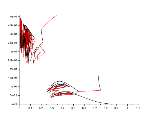
5 Illustrations

We present some numerical simulations illustrating the results of the preceding sections. We consider the environments

$$A_{0}=\left(\begin{array}[]{cc}1&1\\ 2&2\\ \end{array}\right),B_{0}=\left(\begin{array}[]{c}1\\ 5\\ \end{array}\right),$$ (29)

and

$$A_{1}=\left(\begin{array}[]{cc}3&3\\ 4&4+\rho\\ \end{array}\right),B_{1}=\left(\begin{array}[]{c}5\\ 1\\ \end{array}\right).$$ (30)

The simulations below are obtained with

$$\lambda_{0}=st,\lambda_{1}=(1-s)t$$

for different values of $s\in]0,1[,t>0$ and $\rho\in\{0,1,3\}.$ Let $S(u)=\frac{u}{5(1-u)+u}.$ Using, Remark 1, it is easy to check that

(a)

$I=S(]\frac{3}{4}-\frac{1}{2\sqrt{6}},\frac{3}{4}+\frac{1}{2\sqrt{6}}[),$

(b)

$J=I$ for $\rho=0,$

(c)

$J=S(]\frac{71}{96}-\frac{\sqrt{241}}{96},\frac{71}{96}+\frac{\sqrt{241}}{96}[\subset I$ for $\rho=1,$

(d)

$J=\emptyset$ for $\rho=3.$

The phase portraits of $F_{\mathcal{E}_{0}}$ and $F_{\mathcal{E}_{1}}$ are given in Figure 3 with $\rho=3.$

,

Figure 3: Phase portraits of $F_{\mathcal{E}_{0}}$ and $F_{\mathcal{E}_{1}}$

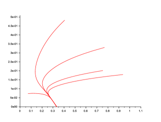
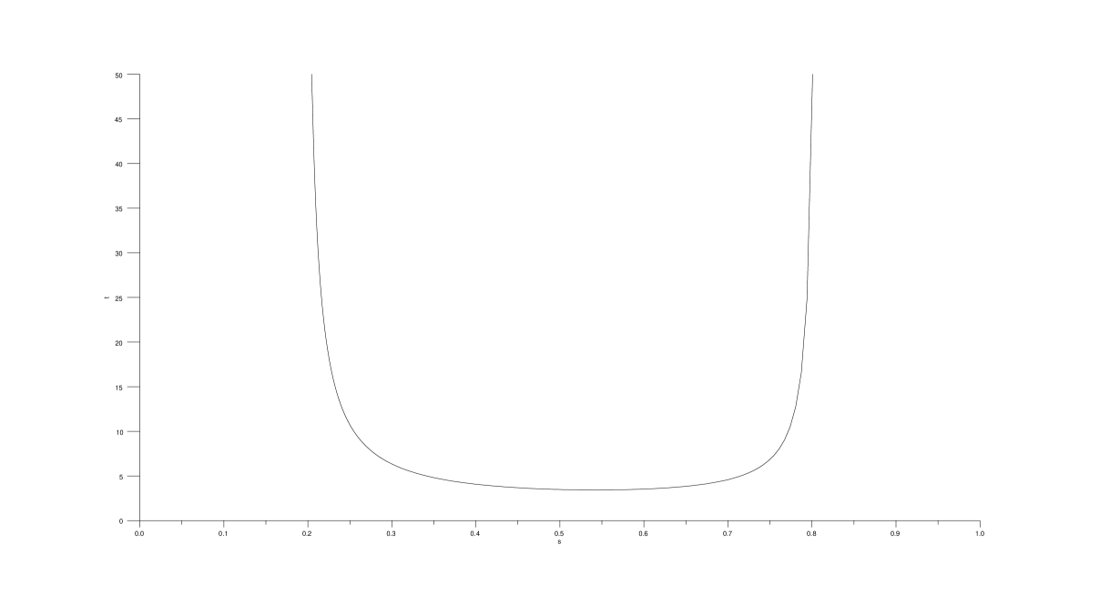
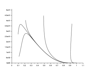
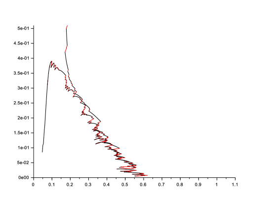
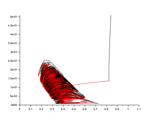
Figure 4 and 5

are obtained with $\rho=3$ (so that $J=\emptyset$). Figure 4 with $s\not\in I$ and $t$ "large" illustrates Theorems 3.1 (extinction of species y). Figure 5 with $s\in I$ illustrates Theorems 4.1 and 4.5 (persistence).

Figure 4: $\rho=3,u=0.4,t=100$ (extinction of species y)

Figure 5: $\rho=3,u=0.75,t=12$ (persistence)

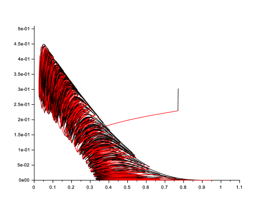
Figures 6 and 7

are obtained with $\rho=1.$ Figure 6 with $s\in I\cap J,t=10$ illustrates Theorems 4.1 and 4.5 (persistence) in case $I\cap J\neq\emptyset.$ Figure 7 with $s\in I\cap J$ and "large" $t$ illustrates Theorem 3.3.

Figure 6: $\rho=1,u=0.75,t=10$ (persistence)

Figure 7: $\rho=1,u=0.75,t=100$ (extinction of species x)

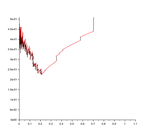
Figures 8

is obtained with $\rho=0$ $s\in I\cap J$ and $t$ conveniently chosen. It illustrates Theorem 3.4.

Figure 8: $\rho=0,u=0.75,t=1/0.15$ (extinction of species x or $y$)

Remark 7

The transitions from extinction of species y to extinction of species x when the jump rate parameter $t$ increases is reminiscent of the transition occurring with linear systems analyzed in [6] and [26].

6 Proofs of Propositions 2.1 and 2.3

6.1 Proof of Proposition 2.1

The process $\{X_{t},Y_{t},I_{t}\}$ restricted to $M_{0}^{\textbf{y}}$ is defined by $Y_{t}=0$ and the one dimensional dynamics

$$\dot{X}=\alpha_{I_{t}}X(1-a_{I_{t}}X)$$ (31)

The invariant probability measure of the chain $(I_{t})$ is given by

$$\nu=\frac{\lambda_{0}}{\lambda_{1}+\lambda_{0}}\delta_{1}+\frac{\lambda_{1}}{\lambda_{1}+\lambda_{0}}\delta_{0}.$$

If $a_{0}=a_{1}=a,X_{t}\rightarrow 1/a=p.$ Thus $(X_{t},I_{t})$ converges weakly to $\delta_{p}\otimes\nu$ and the result is proved.

Suppose now that $0<a_{0}<a_{1}.$

By Proposition 3.17 in [7] and Theorem 1 in [2] ( or Theorem 4.4 in [7]), there exists a unique invariant probability measure $\mu$ on ${\mathbb{R}}_{+}^{*}\times\{0,1\}$ for $(X_{t},I_{t})$ which furthermore is supported by $[p_{1},p_{0}].$ A recent result by [3] also proves that such a measure has a smooth density (in the $x$-variable) on $]p_{1},p_{0}[.$

Let $\Psi:{\mathbb{R}}\times\{0,1\}\mapsto{\mathbb{R}},(x,i)\mapsto\Psi(x,i)$ be smooth in the $x$ variable. Set $\Psi^{\prime}(x,i)=\frac{\partial\Psi(x,i)}{\partial x},$ and $f_{i}(x)=\alpha_{i}x(1-\frac{x}{p_{i}}).$ The infinitesimal generator of $(x(t),I_{t})$ acts on $\Psi$ as follows

$${\cal L}\Psi(x,1) = \langle f_{1}(x),\Psi^{\prime}(x,1)\rangle+\lambda_{1}(\Psi(x,0)-\Psi(x,1))$$

$${\cal L}\Psi(x,0) = \langle f_{0}(x),\Psi^{\prime}(x,0)\rangle+\lambda_{0}(\Psi(x,1)-\Psi(x,0))$$

Write $\mu(dx,1)=h_{1}(x)dx$ and $\mu(dx,0)=h_{0}(x)dx.$ Then

$$\sum_{i=0,1}\int{\cal L}\Psi(x,i)h_{i}(x)dx=0.$$

Choose $\Psi(x,i)=g(x)+c$ and $\Psi(x,1-i)=0$ where $g$ is an arbitrary compactly supported smooth function and $c$ an arbitrary constant. Then, an easy integration by part leads to the differential equation

$$\left\{\begin{array}[]{c}\lambda_{0}h_{0}(x)-\lambda_{1}h_{1}(x)=-(f_{0}h_{0})^{\prime}(x)\\ \lambda_{0}h_{0}(x)-\lambda_{1}h_{1}(x)=(f_{1}h_{1})^{\prime}(x)\end{array}\right.$$ (32)

and the condition

$$\int_{p_{1}}^{p_{0}}\lambda_{0}h_{0}(x)-\lambda_{1}h_{1}(x)dx=0.$$ (33)

The maps

$$h_{1}(x)=C\frac{p_{1}(x-p_{1})^{\gamma_{1}-1}(p_{0}-x)^{\gamma_{0}}}{\alpha_{1}x^{1+\gamma_{1}+\gamma_{0}}},$$ (34)

$$h_{0}(x)=C\frac{p_{0}(x-p_{1})^{\gamma_{1}}(p_{0}-x)^{\gamma_{0}-1}}{\alpha_{0}x^{1+\gamma_{1}+\gamma_{0}}}$$ (35)

are solutions, where $C$ is a normalization constant given by

$$\int_{p_{1}}^{p_{0}}h_{0}(x)+h_{1}(x)dx=1.$$

Note that $h_{1}$ and $h_{0}$ satisfy the equalities:

$$\int_{p_{1}}^{p_{0}}h_{0}(x)dx=\frac{\lambda_{1}}{\lambda_{0}+\lambda_{1}}$$

$$\int_{p_{1}}^{p_{0}}h_{1}(x)dx=\frac{\lambda_{0}}{\lambda_{0}+\lambda_{1}}.$$

This concludes the proof of Proposition 2.1.

6.2 Proof of Proposition 2.3

$(i).$ We assume that $I=\emptyset.$ If $p_{0}=p_{1}$ then $\Lambda_{\textbf{y}}<0.$ Suppose that $a_{0}<a_{1}$ (i.e $p_{0}>p_{1}$) (the proof is similar for $p_{0}<p_{1}$). Let $p_{s}=\frac{1}{a_{s}}$ with $a_{s}$ being given in the definition of $A_{s}.$ The function $s\mapsto p_{s}$ maps $]0,1[$ homeomorphically onto $]p_{0},p_{1}[$ and by definition of $\mathcal{E}_{s}$

$$s\alpha_{1}(1-a_{1}p_{s})+(1-s)\alpha_{0}(1-a_{0}p_{s})=0.$$

Thus $(1-a_{1}p_{s})=-\frac{(1-s)\alpha_{0}}{s\alpha_{1}}(1-a_{0}p_{s}).$ Hence

$$P(p_{s})=\frac{(1-a_{0}p_{s})}{\alpha_{1}s}\beta_{s}(1-c_{s}p_{s})=\frac{\beta_{s}}{\alpha_{1}s}(1-a_{0}/a_{s})(1-c_{s}/a_{s}).$$

This proves that $P(x)\leq 0$ for all $x\in]p_{0},p_{1}[.$ Since $P$ is a nonzero polynomial of degree $2$, $P(x)<0$ for all, but possibly one, points in $]p_{0},p_{1}[.$ Thus $\Lambda_{\textbf{y}}<0.$

$(ii).$ If $a_{0}=a_{1}$ the result is obvious. Thus, we can assume (without loss of generality) that $a_{0}<a_{1}.$ Fix $s\in]0,1[$ and let for all $t>0$ $\nu_{1}^{t}$ (respectively $\nu_{0}^{t}$) be the probability measure defined as $\nu_{1}^{t}(dx)=\frac{1}{s}h_{1}^{t}(x){\mathbf{1}}_{]p_{1},p_{0}[}(x)dx$ ($\nu_{0}^{t}(dx)=\frac{1}{1-s}h_{0}^{t}(x){\mathbf{1}}_{]p_{1},p_{0}[}(x)dx$) where $h_{1}^{t}$ (respectively $h_{0}^{t}$) is the map defined by equation (34) (respectively (35)) with $\lambda_{0}=st$ and $\lambda_{1}=(1-s)t.$ We shall prove that

$$\nu_{i}^{t}\Rightarrow\delta_{p_{s}}\mbox{ as }t\rightarrow\infty$$ (36)

and

$$\nu_{i}^{t}\Rightarrow\delta_{p_{i}}\mbox{ as }t\rightarrow 0,$$ (37)

where $\Rightarrow$ denotes the weak convergence. The result to be proved follows.

Let us prove (36). For all $x\in]p_{0},p_{1}[,\nu_{i}^{t}(dx)=C^{t}_{i}e^{tW(x)}[x|x-p_{i}|]^{-1}{\mathbf{1}}_{]p_{1},p_{0}[}(x)dx$ where $C^{t}_{i}$ is a normalization constant and

$$W(x)=\frac{s}{\alpha_{0}}\log(p_{0}-x)+\frac{1-s}{\alpha_{1}}\log(x-p_{1})-\frac{\alpha_{s}}{\alpha_{0}\alpha_{1}}\log(x).$$

We claim that

$$argmax_{]p_{0},p_{1}[}W=p_{s}=\frac{1}{a_{s}}$$ (38)

Indeed, set $Q(x)=W^{\prime}(x)(\alpha_{0}\alpha_{1}x((x-p_{0})(p_{1}-x)).$ It is easy to verify that

$$Q(x)=s\alpha_{1}(p_{1}-x)x-(1-s)\alpha_{0}(x-p_{0})x-\alpha_{s}(p_{0}-x)(x-p_{1}).$$

Thus $Q(p_{0})<0,Q(p_{1})>0$ and since $Q$ is a second degree polynomial, it suffices to show that $Q(p_{s})=0$ to conclude that $p_{s}$ is the global minimum of $W.$ By definition of $p_{s},$

$$s\alpha_{1}(1-a_{1}p_{s})+(1-s)\alpha_{0}(1-a_{0}p_{s})=0.$$

Thus

$$(1-s)\alpha_{0}(p_{s}-p_{0})=\frac{s\alpha_{1}a_{1}}{a_{0}}(p_{1}-p_{s}).$$

Plugging this equality in the expression of $Q(p_{s})$ leads to $Q(p_{s})=0.$ This proves the claim. Now, from equation (38) and Laplace principle we deduce (36).

We now pass to the proof of (37). It suffices to show that $\nu_{i}^{t}$ converges in probability to $p_{i},$ meaning that $\nu_{i}^{t}\{x:\>|x-p_{i}|\geq\varepsilon\}\rightarrow 0$ as $t\rightarrow 0.$ This easily follows from the shape of $h_{i}^{t}$ and elementary estimates. $\Box$

References

- [1] P. A. Abrams, R. D. Holt, and J. D. Roth, Apparent competition of apparent mutualism? shared predation when population cycles, Ecology 79 (1998), 202–212.
- [2] Y. Bakhtin and T. Hurth, Invariant densities for dynamical systems with random switching, Nonlinearity (2012), no. 10, 2937–2952.
- [3] Y. Bakhtin, T. Hurth, and J.C. Mattingly, Regularity of invariant densities for 1d-systems with random switching, Preprint 2014, http://arxiv.org/abs/1406.5425.
- [4] M. Benaïm, Stochastic persistence, Preprint, 2014.
- [5] M. Benaïm, J. Hofbauer, and W. Sandholm, Robust permanence and impermanence for the stochastic replicator dynamics, Journal of Biological Dynamics 2 (2008), no. 2, 180–195.
- [6] M. Benaïm, S. Le Borgne, F. Malrieu, and P-A. Zitt, On the stability of planar randomly switched systems, Annals of Applied Probabilities (2014), no. 1, 292–311.
- [7] , Qualitative properties of certain piecewise deterministic markov processes, Annales de l’IHP 51 (2015), no. 3, 1040 – 1075, http://arxiv.org/abs/1204.4143.
- [8] O. Boxma, H. Kaspi, O. Kella, and D. Perry, On/Off Storage Systems with State-Dependent Inpout, Outpout and Swithching Rates, Probability en the Engineering and Informational Siences 19 (2005), 1–14.
- [9] P. L. Chesson, The stabilizing effect of a random environment, Journal of Mathematical Biology 15 (1982), 1–36.
- [10] , Mechanisms of maintenance of species diversity, Annual Review of Ecology and Systematics 31 (2000), 343–366.
- [11] P. L. Chesson and S. Ellner, Invasibility and stochastic boundedness in monotonic competition models, Journal of Mathematical Biology 27 (1989), 117–138.
- [12] P. L. Chesson and R.R. Warner, Environmental variability promotes coexistence in lottery competitive systems, American Naturalist 117 (1981), no. 6, 923–943.
- [13] J. M. Cushing, Two species competition in a periodic environment, J. Math. Biology (1980), 385–400.
- [14] P. de Mottoni and A. Schiaffino, Competition systems with periodic coefficients: A geometric approach, J. Math. Biology (1981), 319–335.
- [15] S. N. Evans, A. Hening, and S. J. Schreiber, Protected polymorphisms and evolutionary stability of patch-selection strategies in stochastic environments, Journal of Mathematical Biology 71 (2015), 325–359.
- [16] B. M. Garay and J. Hofbauer, Robust permanence for ecological equations, minimax, and discretization, Siam J. Math. Anal. Vol. 34 (2003), no. 5, 1007–1039.
- [17] G. F. Gause, Experimental studies on the struggle for existence, Journal of Experimental Biology (1932), 389–402.
- [18] M. Hairer and J. Mattingly, Yet another look at harris ergodic theorem for markov chains, Seminar on Stochastic Analysis, Random Fields and Applications VI (Dalang, ed.), Progress in Probability, 2011, pp. 109–117.
- [19] G. Hardin, Competitive exclusion principle, Science (1960), 1292–1297.
- [20] M. W. Hirsch and H. Smith, Monotone dynamical systems, Handbook of Differential Equations (A Cañada, P Drábek, and A Fonda, eds.), vol. 2, ELSEVIER, 2005.
- [21] J. Hofbauer, A general cooperation theorem for hypercycles, Monatshefte fur Mathematik (1981), no. 91, 233–240.
- [22] J. Hofbauer and S. Schreiber, To persist or not to persist , Nonlinearity 17 (2004), 1393–1406.
- [23] J. Hofbauer and K. Sigmund, Evolutionary games and population dynamics, Cambridge University Press, 1998.
- [24] G. E. Hutchinson, The paradox of the plankton, The American Naturalist 95 (1961), no. 882, 137–145.
- [25] A. L. Koch, Coexistence resulting from an alternation of density dependent and density independent growth, J. Theor. Biol. 44 (1974), 373–3.
- [26] S. D. Lawley, J. C. Mattingly, and M. C. Reed, Sensitivity to switching rates in stochastically switched odes, Preprint 2012, http://arxiv.org/abs/1310.2525v1.
- [27] C. Lobry, A. Sciandra, and P. Nival, Effets paradoxaux des fluctuations de l’environnement sur la croissance des populations et la compétition entres espèces, C.R. Acad. Sci. Paris, Life Sciences (1994), 317:102–7.
- [28] F. Malrieu and P. A. Zitt, On the persistence regime for lotka-volterra in randomly fluctuating environments, Preprint, http://arxiv.org/abs/1601.08151, 2016.
- [29] S. Schreiber, Criteria for robust permanence, J Differential Equations (2000), 400–426.
- [30] , Persistence for stochastic difference equations: A mini review, Journal of Difference Equations and Applications 18 (2012), 1381–1403.
- [31] S. Schreiber, M. Bena m, and K. A. S. Atchad , Persistence in fluctuating environments, Journal of Mathematical Biology 62 (2011), 655–683.
- [32] H. L. Smith and H. R. Thieme, Dynamical systems and population persistence, vol. 118, American Mathematical Society, Providence, RI, 2011.
- [33] M. Turelli, Does environmental variability limit niche overlap ?, Proc. Natl. Acad. Sci. 75 (1978), 5085–5089.
Acknowledgments
This work was supported by the SNF grants FN 200020-149871/1 and 200021-163072/1 We thank Mireille Tissot-Daguette for her help with Scilab, Elisa Gorla for her help with Maclau2 and three anonymous referees for their useful comments and recommendations on the first version of this paper.