Herschel Survey of Galactic OH⁺, H₂O⁺, and H₃O⁺: Probing the Molecular Hydrogen Fraction and Cosmic-Ray Ionization Rate.

Abstract

In diffuse interstellar clouds the chemistry that leads to the formation of the oxygen bearing ions OH⁺, H₂O⁺, and H₃O⁺ begins with the ionization of atomic hydrogen by cosmic rays, and continues through subsequent hydrogen abstraction reactions involving H₂. Given these reaction pathways, the observed abundances of these molecules are useful in constraining both the total cosmic-ray ionization rate of atomic hydrogen ($\zeta_{\rm H}$) and molecular hydrogen fraction ($f_{\rm H_{2}}$). We present observations targeting transitions of OH⁺, H₂O⁺, and H₃O⁺ made with the Herschel Space Observatory along 20 Galactic sight lines toward bright submillimeter continuum sources. Both OH⁺ and H₂O⁺ are detected in absorption in multiple velocity components along every sight line, but H₃O⁺ is only detected along 7 sight lines. From the molecular abundances we compute $f_{\rm H_{2}}$ in multiple distinct components along each line of sight, and find a Gaussian distribution with mean and standard deviation $0.042\pm 0.018$. This confirms previous findings that OH⁺ and H₂O⁺ primarily reside in gas with low H₂ fractions. We also infer $\zeta_{\rm H}$ throughout our sample, and find a log-normal distribution with mean $\log(\zeta_{\rm H})=-15.75$, ($\zeta_{\rm H}=1.78\times 10^{-16}$ s^-1), and standard deviation 0.29 for gas within the Galactic disk, but outside of the Galactic center. This is in good agreement with the mean and distribution of cosmic-ray ionization rates previously inferred from H${}_{3}^{+}$ observations. Ionization rates in the Galactic center tend to be 10–100 times larger than found in the Galactic disk, also in accord with prior studies.

1 INTRODUCTION

Astrochemistry is a flourishing field, with over 180 molecules (300 when accounting for isotopologues) detected in interstellar and circumstellar environments (Lovas & Snyder, 2014). Several of the more recent detections, including those of OH⁺ (Wyrowski et al., 2010a) and H₂O⁺ (Ossenkopf et al., 2010), were made possible as new technology has pushed both ground and space-based observatories into the THz frequency range. Of particular importance was the Herschel Space Observatory (Pilbratt et al., 2010), which offered a view of the THz regime unimpeded by atmospheric absorption. As the inventory of interstellar molecules and complexity of chemical reaction networks grow, it remains imperative that we are able to select the most important reactions governing the abundance of a particular species, and understand how observations of closely related species can be utilized to infer properties of the interstellar medium (ISM).

A basic understanding of how the chemistry involving different species proceeds in the ISM can be garnered from knowledge of a few key atomic and molecular properties, one of which is the first ionization potential (FIP). Neutral-neutral reactions proceed slowly at the relatively low temperatures in diffuse clouds, while ion-neutral reactions are typically much faster and so dominate diffuse cloud chemistry. This necessitates an external ionization mechanism to drive the reaction network. Species with FIP less than 13.6 eV (below the ionization potential of atomic hydrogen) can be photoionized by far-ultraviolet photons from the interstellar radiation field, and will predominantly be in ionized form. For species with FIP above 13.6 eV, atomic hydrogen effectively absorbs the ionizing interstellar radiation field, and they remain predominantly in neutral form. Reaction networks of such species are generally initiated by reactions with the ions H⁺ and H${}_{3}^{+}$—both of which are primarily formed via cosmic-ray ionization of H and H₂, respectively—and so the chemistry surrounding these species can be considered cosmic-ray driven. Oxygen falls into this latter category ($\mathrm{FIP}=13.62$ eV), so the abundances of various oxygen-bearing molecules are closely linked to the cosmic-ray ionization rate.

Another controlling parameter is the bond-dissociation energy, $D_{0}$. If $D_{0}>4.48$ eV (dissociation energy of H₂) for a species XH⁺, then the reaction $\mathrm{X^{+}+H_{2}\rightarrow XH^{+}+H}$ is exothermic. This is especially important for interstellar chemistry at low temperatures, where there is little kinetic energy to aid in reactions. Dissociation energies of OH⁺, H₂O⁺, and H₃O⁺ are all greater than 4.48 eV, and O⁺, OH⁺, and H₂O⁺ all react exothermically with H₂. As H₂ is the most abundant molecule in the universe, the abundances of these molecular ions—specifically with respect to each other—are highly dependent on the amount of H₂ available for reactions.

The properties of O and oxygen-bearing ions described above explain the particular utility of OH⁺, H₂O⁺, and H₃O⁺ in constraining conditions in the ISM. The formation of each larger molecule requires one more hydrogen abstraction reaction with H₂, a process that competes primarily with dissociative recombination with electrons in destroying these ions. This makes the ratios $n({\rm H_{2}O^{+}})/n({\rm H_{3}O^{+}})$ and $n({\rm OH^{+}})/n({\rm H_{2}O^{+}})$ sensitive to the ratio $n(e)/n({\rm H_{2}})$. If the fractional abundance of electrons with respect to total hydrogen ($x_{e}\equiv n(e)/n_{\rm H}$, where $n_{\rm H}\equiv n({\rm H})+2n({\rm H_{2}})$) is known, then these ratios can also be used to infer the molecular hydrogen fraction, $f_{\rm H_{2}}\equiv 2n({\rm H_{2}})/n_{\rm H}$. Initial results from observations of OH⁺ and H₂O⁺ along the sight lines toward W49N and W31C showed $f_{\rm H_{2}}\lesssim 0.1$, implying that both species reside in gas that is primarily atomic (Gerin et al., 2010b; Neufeld et al., 2010). This conclusion is supported by the distribution of OH⁺ and H₂O⁺ absorption in velocity space, which more closely matches that of atomic H than that of H₂O and HF (both tracers of molecular gas). Similar results are found from observations of electronic transitions of OH⁺ in the ultraviolet, as it is better correlated with CH⁺ than with species tracing denser molecular gas such as CH, CN, and OH (Krełowski et al., 2010; Porras et al., 2014). In many sight lines, absorption of OH⁺ and H₂O⁺ arises at or near the systemic velocity of the background source as well, and is thought to trace the irradiated outflows near massive protostars. Even for these objects though, the OH⁺/H₂O⁺ and H₂O/H₂O⁺ ratios are interpreted as indicating relatively low-density, mostly atomic gas (Benz et al., 2010; Bruderer et al., 2010; Wyrowski et al., 2010b). Only rarely have OH⁺ and H₂O⁺ column densities required high molecular fractions (e.g., Orion KL; Gupta et al., 2010).

As the formation of OH⁺ in diffuse gas begins with the ionization of H by cosmic rays, its abundance is useful in constraining the cosmic-ray ionization rate of atomic hydrogen, $\zeta_{\rm H}$. While other molecules are also used for this purpose, OH⁺ is unique in its ability to probe $\zeta_{\rm H}$ in gas with $0.01\lesssim f_{\rm H_{2}}\lesssim 0.1$. Estimates of the cosmic-ray ionization rate in diffuse clouds based on molecular abundances have been made for roughly 40 years now, with the earliest utilizing observations of OH and HD in diffuse clouds (O’Donnell & Watson, 1974; Black & Dalgarno, 1977; Black et al., 1978; Hartquist et al., 1978). Those studies typically found ionization rates on the order of a few times 10^-17 s^-1, as did later studies using the same molecules (Federman et al., 1996), although van Dishoeck & Black (1986) required ionization rates of a few times 10^-16 s^-1 to reproduce observed column densities with a more detailed model. Findings were generally in good agreement with estimates of $\zeta_{\rm H}$ based on the local interstellar proton spectrum measured by Voyager (Webber, 1998). As a result, it was thought that the cosmic-ray ionization rate was relatively uniform throughout the Galaxy, and a canonical value of $\zeta_{\rm H}=3\times 10^{-17}$ s^-1 was frequently adopted.

The detection of H${}_{3}^{+}$ in the ISM (Geballe & Oka, 1996) introduced a new, less complicated tracer of the ionization rate, and subsequent surveys of H${}_{3}^{+}$ pointed to an ionization rate in diffuse clouds nearly ten times larger than that found previously: $\zeta_{\rm H}\approx 2\times 10^{-16}$ s^-1 (McCall et al., 2003; Indriolo et al., 2007; Indriolo & McCall, 2012). In addition, the distribution of ionization rates inferred from H${}_{3}^{+}$ was found to vary by over 1 order of magnitude, suggesting that the low-energy cosmic-ray flux is not uniform throughout the Galaxy. It now seems likely that most early estimates of $\zeta_{\rm H}$ were too low because they assumed that nearly every instance of hydrogen being ionized by a cosmic ray led to the formation of OH or HD. However, destruction of H⁺ by polycyclic aromatic hydrocarbons (PAHs) and small grains is highly competitive with the charge transfer reactions driving the oxygen and deuterium chemistries (Wolfire et al., 2003), making the chemical pathways from H⁺ to OH and HD “leaky.” This mechanism was recognized by Liszt (2003) as a way to reconcile the differences in ionization rates inferred from OH and HD with those inferred from H${}_{3}^{+}$. Neutralization of H⁺ on grains is also important in the chemistry leading to OH⁺ and H₂O⁺, and its effects are now accounted for when using these species to infer the ionization rate (Neufeld et al., 2010; Hollenbach et al., 2012; Indriolo et al., 2012).

While infrared and radio observations of interstellar molecules—carefully interpreted in the context of astrochemical models—can be used to determine the density of low-energy cosmic rays ($E\lesssim 10$ MeV), gamma-ray observations provide a complementary probe of high-energy cosmic rays ($E\gtrsim 300$ MeV). The latter interact with atomic nuclei in the interstellar gas, producing neutral pions ($\pi^{0}$) that rapidly decay into pairs of gamma-ray photons (Beringer et al., 2012). Observations of these gamma-rays can be used to estimate the density of high-energy cosmic rays as a function of location within the Galaxy. Our understanding of the gamma-ray sky has greatly improved following the launch of the Fermi Gamma-ray Space Telescope, with recent observations of the outer Galaxy suggesting that the cosmic-ray density is relatively uniform outside the solar circle, and declines less rapidly with Galactocentric radius ($R_{\rm gal}$) than predicted by propagation models (Ackermann et al., 2011). An interesting question is whether the density of low-energy particles shows the same behavior, or whether the significantly smaller amount of material through which such particles can travel before losing all of their energy leads to a different result.

Observations of H${}_{3}^{+}$ have primarily been limited to the local ISM (within about 2 kpc of the Sun; McCall et al., 2002; Indriolo & McCall, 2012) due to the necessity for high spectral resolution and high continuum level signal-to-noise ratio (S/N). The most notable exceptions have been ongoing surveys of the Galactic center region which reveal a large amount of warm, diffuse gas that experiences a large flux of cosmic rays, with ionization rates above $10^{-15}$ s^-1 (Oka et al., 2005; Goto et al., 2008, 2011; Geballe & Oka, 2010). Even the dense gas in the Galactic center experiences a cosmic-ray ionization rate 10–100 times larger than the dense gas elsewhere in the Galactic disk, as determined from observations of H₃O⁺, H¹³CO⁺, and H${}_{3}^{+}$ (van der Tak & van Dishoeck, 2000; van der Tak et al., 2006; Goto et al., 2013, 2014), suggesting an increased particle flux in the Galactic center at all energies. Still, all of these observations have only probed ionization rates in the Galactic center and the local ISM. To expand this coverage to wider portions of the Galaxy and answer the question posed above, other tracers of the cosmic-ray ionization rate are needed, and Herschel provided the opportunity to use observations of OH⁺ and H₂O⁺ for this purpose.

1.1 Oxygen Chemistry

Oxygen chemistry in diffuse clouds is thought to be relatively simple (e.g., Hollenbach et al., 2012), with the network of ion-neutral reactions initiated by the ionization of atomic hydrogen by cosmic rays,

$${\rm H}+{\rm CR}\rightarrow{\rm H}^{+}+e^{-}+{\rm CR^{\prime}}.$$ (1)

Ionization of H is followed by endothermic charge transfer to oxygen to form O⁺,

$${\rm H}^{+}+{\rm O}+\Delta E\longleftrightarrow{\rm O}^{+}+{\rm H},$$ (2)

where $\Delta E=226$ K represents the endothermicity of the forward reaction (for O in the lowest energy fine-structure level, ${}^{3}P_{2}$, of the ground state), and the double-sided arrow shows that the exothermic back-reaction proceeds uninhibited. The rate of the forward reaction for oxygen in each of the ${}^{3}P_{J}$ ($J=0,1,2$) fine-structure levels is highly dependent on the gas kinetic temperature (about 100 K on average in diffuse clouds), and the total forward rate on the relative population in the fine-structure levels of atomic oxygen (Stancil et al., 1999). Also, the O in reaction (2) competes with electrons and neutral and charged small grains and PAHs in destroying H⁺ (Wolfire et al., 2003),

$${\rm H}^{+}+{\rm PAH} \rightarrow{\rm H}+{\rm PAH}^{+},$$

$${\rm H}^{+}+{\rm PAH}^{-} \rightarrow{\rm H}+{\rm PAH},$$

$${\rm H}^{+}+e^{-} \rightarrow{\rm H}+h\nu,$$

all of which decrease the efficiency at which ionization of H leads to the formation of OH⁺ (Liszt, 2003). Once O⁺ is formed it can undergo the back-reaction with H, or it can react with H₂ to form OH⁺,

$$\mathrm{O^{+}+H_{2}\rightarrow OH^{+}+H},$$ (3)

which is either destroyed by further hydrogen abstraction to form H₂O⁺,

$$\mathrm{OH^{+}+H_{2}\rightarrow H_{2}O^{+}+H},$$ (4)

or by dissociative recombination with electrons,

$$\mathrm{OH^{+}}+e^{-}\rightarrow\mathrm{products}.$$ (5)

The same is true for H₂O⁺,

$$\mathrm{H_{2}O^{+}+H_{2}\rightarrow H_{3}O^{+}+H},$$ (6)

$$\mathrm{H_{2}O^{+}}+e^{-}\rightarrow\mathrm{products},$$ (7)

but H₃O⁺ is primarily destroyed by dissociative recombination with electrons,

$$\mathrm{H_{3}O^{+}}+e^{-}\rightarrow\mathrm{products},$$ (8)

as further hydrogen abstraction reactions with H₂ do not proceed. It is apparent from reactions (3) through (8) that the abundances of these species are controlled by competition between hydrogen abstraction from H₂ and dissociative recombination with electrons.

In addition to reaction (3), it is possible for the oxygen chemistry to be driven by the reaction

$${\rm O}+{\rm H_{3}^{+}}\rightarrow{\rm OH}^{+}+{\rm H_{2}},$$ (9)

where H${}_{3}^{+}$ is formed following cosmic-ray ionization of H₂ and subsequent reaction of H${}_{2}^{+}$ with another H₂. To compete with reactions (1)–(3), this pathway requires a substantial fraction of hydrogen to be in molecular form. In gas with small $f_{\rm H_{2}}$, cosmic-ray ionization will produce significantly more H⁺ than H${}_{2}^{+}$. Additionally, H${}_{2}^{+}$ is likely to undergo charge exchange with the abundant H (i.e., $\rm{H}_{2}^{+}+{\rm H}\rightarrow{\rm H}_{2}+{\rm H}^{+}$), prior to finding another H₂, limiting the formation of H${}_{3}^{+}$. Combined, these two effects inhibit the pathway to OH⁺ through reaction (9) in gas that is mostly atomic. As we will show that most of the gas under consideration in this study is diffuse with low molecular hydrogen fraction, we omit this formation route from our analysis, and focus instead on the pathway following reactions (1)–(3).

The utility of OH⁺ and H₂O⁺ abundances in constraining the molecular hydrogen fraction and cosmic-ray ionization rate has been demonstrated in multiple studies (e.g., Gerin et al., 2010b; Neufeld et al., 2010; Indriolo et al., 2012), and makes observations of these species important for studying properties of the diffuse Galactic ISM. As part of the PRISMAS (PRobing InterStellar Molecules with Absoprtion line Studies) Key Program, and motivated by the astrochemical and astrophysical considerations discussed above, we carried out a survey of OH⁺ and H₂O⁺ line absorption toward nine bright submillimeter continuum sources using the Heterodyne Instrument for the Far-Infrared (HIFI; de Graauw et al., 2010) on Herschel. The target sources all lie in the Galactic plane, and are all known to exhibit absorption by molecules in foreground molecular clouds not associated with the sources themselves. Results from three of the targeted sight lines—W31C, W49N, and W51e—have been reported previously, but those studies only utilized a portion of the data that are now available. In this paper we have compiled the full set of observations of OH⁺ and H₂O⁺ from PRISMAS, as well as observations from other Herschel programs toward 11 more sight lines with the intent of exploring $f_{\rm H_{2}}$ and $\zeta_{\rm H}$ throughout the Galaxy. The sample of observations is described in Section 2; the analysis of these data and findings in Section 3; and a discussion of the findings in Section 4.

2 OBSERVATIONS

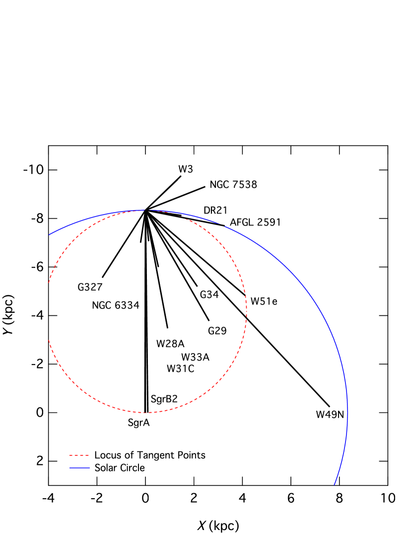
Figure 1: Distribution of observed sight lines as viewed from the North Galactic Pole. Many source names have been shortened for clarity. The Galactic center is located at (0,0), and the Sun is assumed to be 8.34 kpc away (Reid et al., 2014). The blue solid curve shows the solar circle, and the red dashed curve the locus of tangent velocities. Only the W49N line of sight significantly samples both near and far kinematic distances, leading to severe blending of absorption features arising in physically separated clouds.

All observations presented herein were made using the HIFI instrument on board Herschel. Multiple transitions of the oxygen-bearing ions OH⁺, H₂O⁺, and H₃O⁺ were targeted in several different observing programs. A list of the targeted transitions is given in Table 1. Sight lines along which observations were made are listed in Table 2, and Figure 1 shows their distribution in the Galactic disk. Observations were performed using the dual beam switch mode, with the telescope beam centered at the coordinates given in Table 2, and the reference positions located at offsets of 3′ on either side of each source. Multiple local oscillator (LO) frequencies separated by small offsets were used to confirm the assignment of any observed spectral feature to either the upper or lower sideband of the double sideband HIFI receivers. All data were acquired using the Wide Band Spectrometer, which provides a spectral resolution of 1.1 MHz and a bandwidth of $\sim 4$ GHz. As discussed in Neufeld et al. (2010), the data were processed using the standard HIFI pipeline (versions 9.1 through 11.1 depending on when data were downloaded) to Level 2, providing fully calibrated spectra with the intensities expressed as antenna temperature. The resultant spectra were co-added to recover the signal-to-noise ratio that would have been obtained at a single LO setting. Spectra obtained for the horizontal and vertical polarizations were found to be very similar in their appearance and noise characteristics and were likewise coadded.

3 ANALYSIS AND RESULTS

3.1 Spectra

Table 3 lists the double sideband (DSB) continuum antenna temperature, $T_{A}({\rm DSB})$, measured for each of the target sources at the relevant observing frequencies, together with the root mean square (RMS) noise in the co-added spectra. Because HIFI employs double sideband receivers, the complete absorption of radiation in any observed spectral line reduces the antenna temperature to roughly one-half its continuum value. The fractional transmission at any frequency is given by

$$\frac{F(\nu)}{F({\rm cont})}=\left[T_{A}(\nu)-\frac{T_{A}({\rm DSB})}{(1+\Gamma)}\right]\left[\frac{T_{A}({\rm DSB})}{(1+\Gamma^{-1})}\right]^{-1},$$ (10)

where $\Gamma$ is defined as the continuum antenna temperature coming from the sideband containing the frequency of interest divided by the continuum antenna temperature coming from the opposite sideband. In the special case with $\Gamma=1$, i.e., both sidebands contribute equally to $T_{A}({\rm DSB})$, equation (10) simplifies to $F(\nu)/F({\rm cont})=2T_{A}(\nu)/T_{A}({\rm DSB})-1$. For all transitions of H₂O⁺ and H₃O⁺, and for the 909 GHz and 1033 GHz transitions of OH⁺ $\Gamma=1$ is adopted in converting spectra from antenna temperature to fractional transmission (justified by measurements of sideband ratios reported in Higgins et al., 2014). In cases where absorption by the 971 GHz transition of OH⁺ is saturated, the relative intensities of the different hyperfine components of the transition are assumed constant, and the measured optical depth of the weakest component is used to predict the optical depth of the strongest component. This enables the determination of $\Gamma$, and is an important step as small changes in saturated absorption correspond to large differences in optical depth and thus inferred column density.

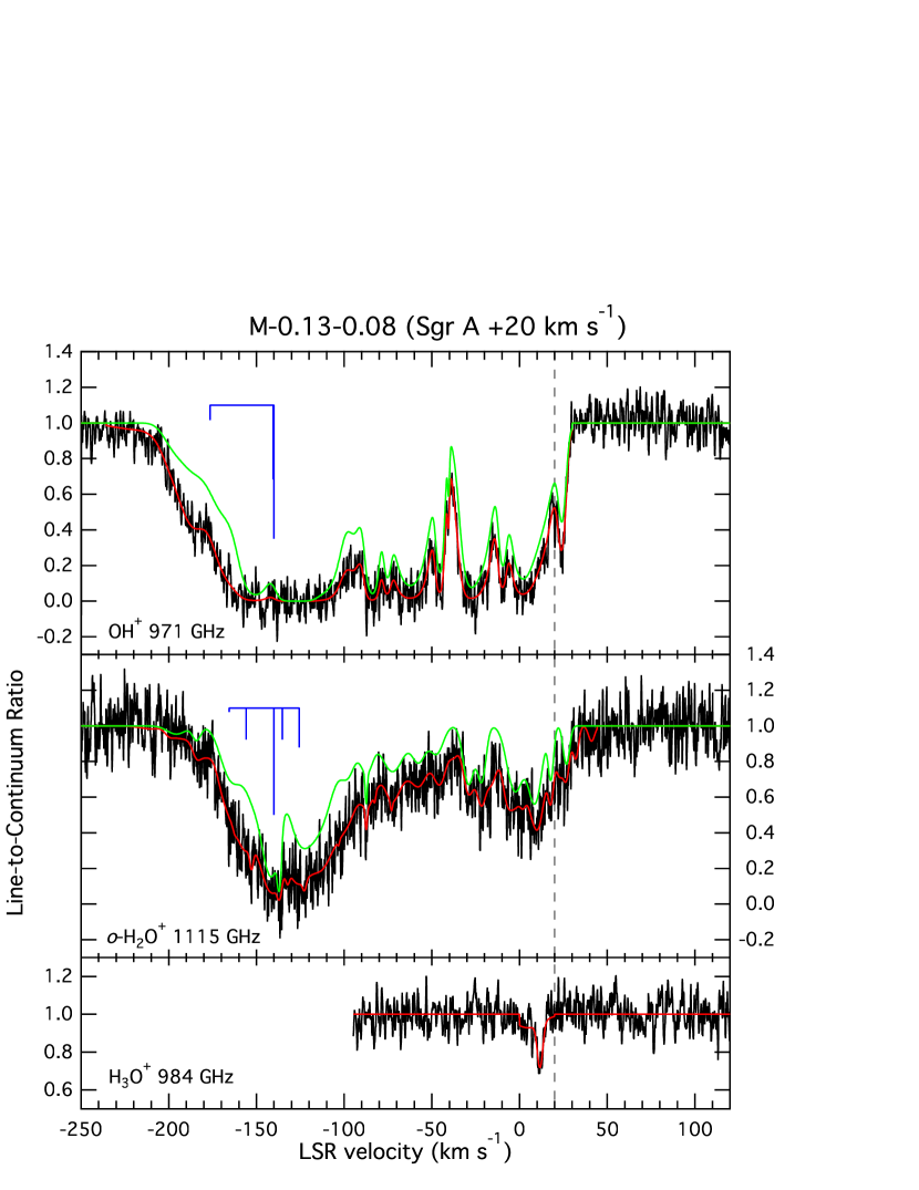
Figure 2: Single sideband normalized spectra toward M$-$0.13$-$0.08 (SgrA $+$20 km s^-1 cloud) showing transitions of OH⁺, H₂O⁺, and H₃O⁺. Stick diagrams above spectra show the hyperfine structure where applicable. Red curves are fits to the absorption features, and green curves show only the strongest hyperfine component of the fits. The vertical dashed line marks the systemic velocity of the background source. Vertical axes give line-to-continuum ratio, with labels alternating between the left and right sides for clarity.

The resulting spectra for all observed transitions and sources are presented in Figures 2 through 21. OH⁺ and the ortho spin modification of H₂O⁺ are detected in absorption toward all of the targeted sight lines, while H₃O⁺ and the para form of H₂O⁺ are each seen in absorption toward only 7 sight lines. Fits to the absorption features (fitting procedure described below) are shown as red curves (blue curves for the sight lines toward Sgr B2), and for transitions with hyperfine splitting the green curves show only absorption due to the strongest hyperfine component. Stick diagrams above spectra mark the hyperfine structure when applicable.

3.2 Spectral Fitting

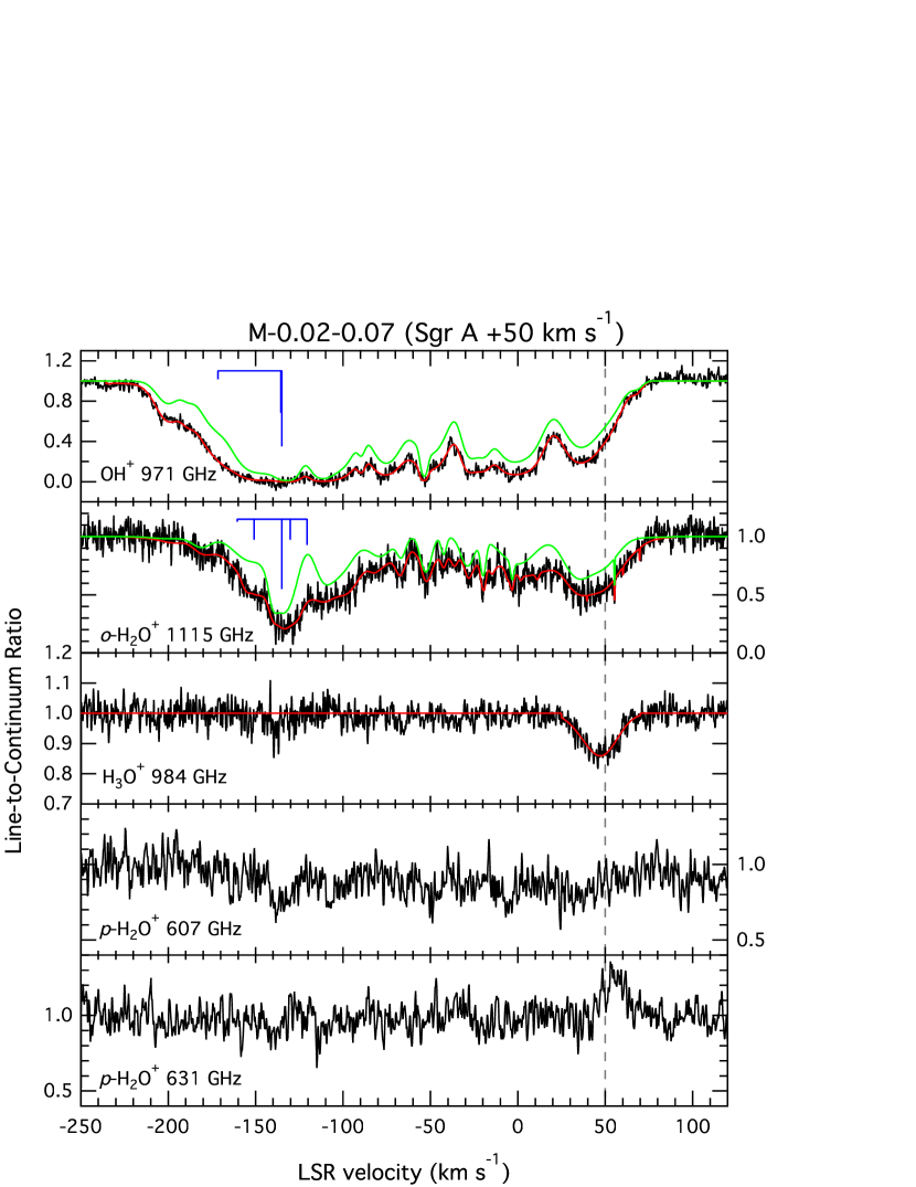
Figure 3: Same as Figure 2 but for M$-$0.02$-$0.07 (SgrA $+$50 km s^-1 cloud).

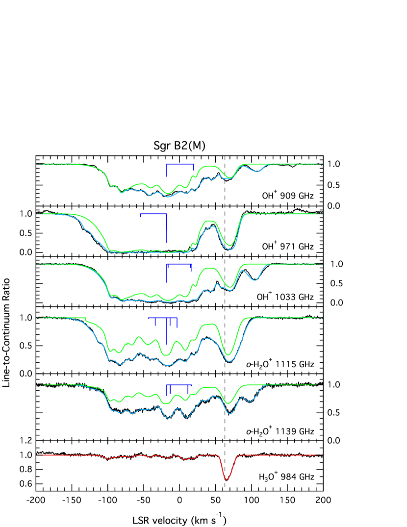
Figure 4: Same as Figure 2 but for Sgr B2(M). In this case, however, fits shown by blue curves were made by using absorption from all relevant transitions (e.g., 909 GHz, 971 GHz, and 1033 GHz transitions of OH⁺) simultaneously.

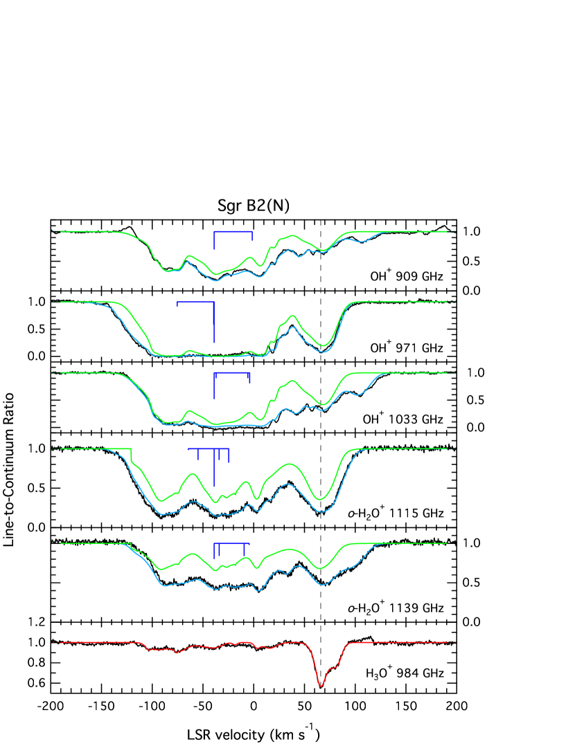
Figure 5: Same as Figure 4 but for Sgr B2(N).

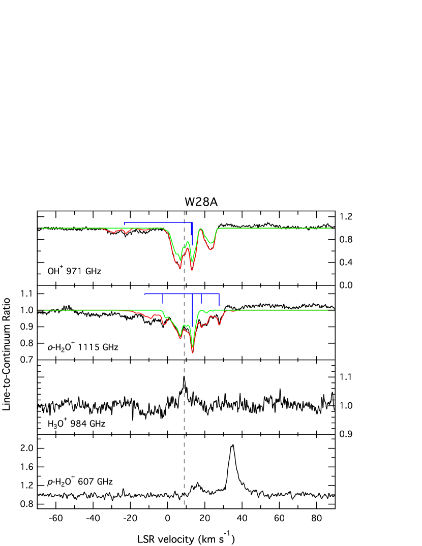
Figure 6: Same as Figure 2 but for W28A.

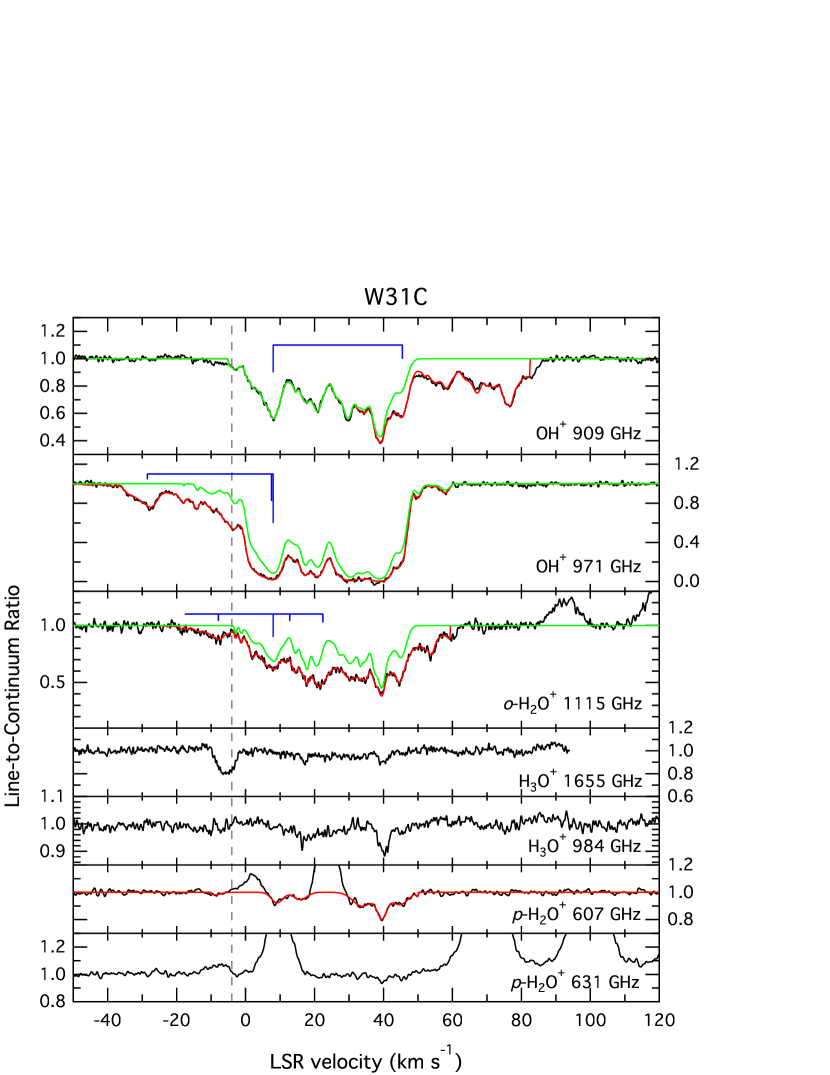
Figure 7: Same as Figure 2 but for W31C.

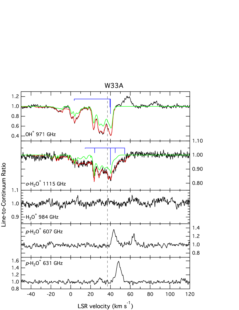
Figure 8: Same as Figure 2 but for W33A.

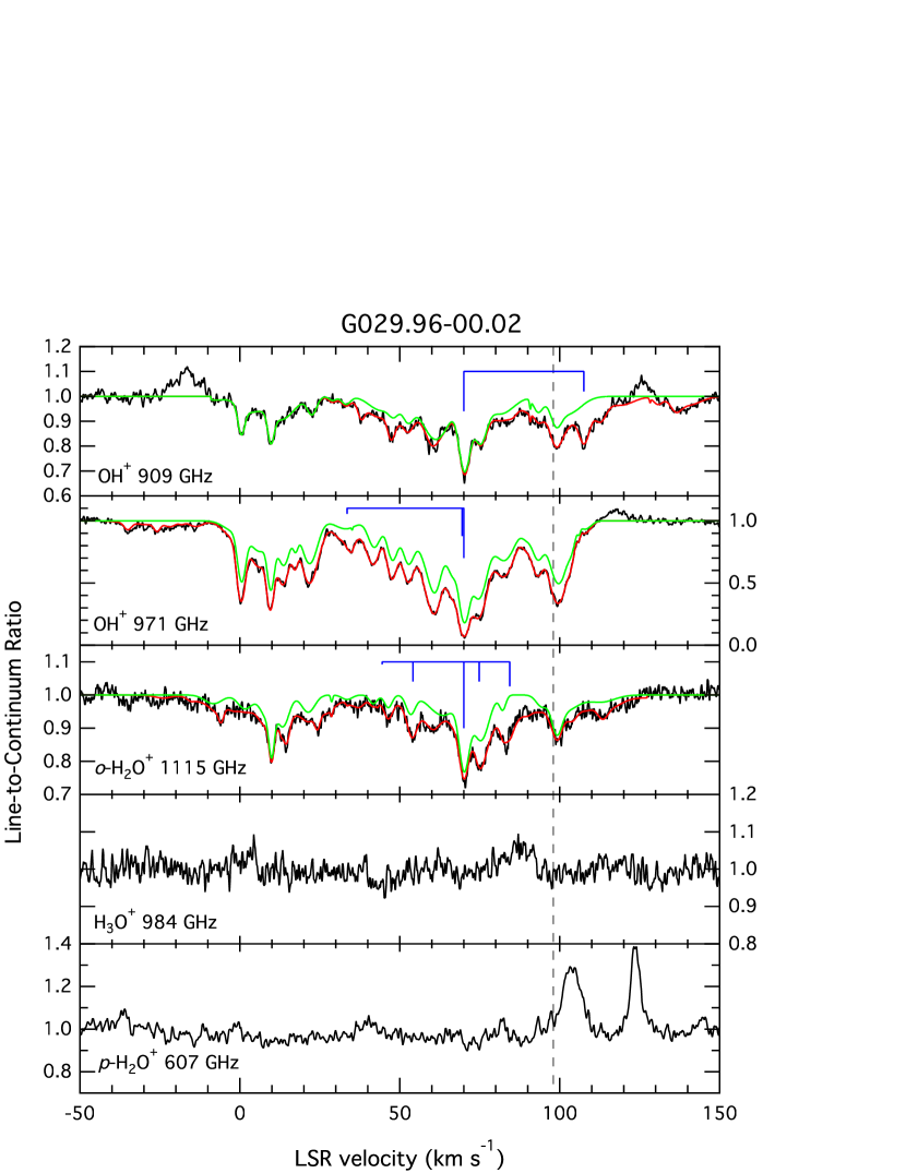
Figure 9: Same as Figure 2 but for G029.96$-$00.02.

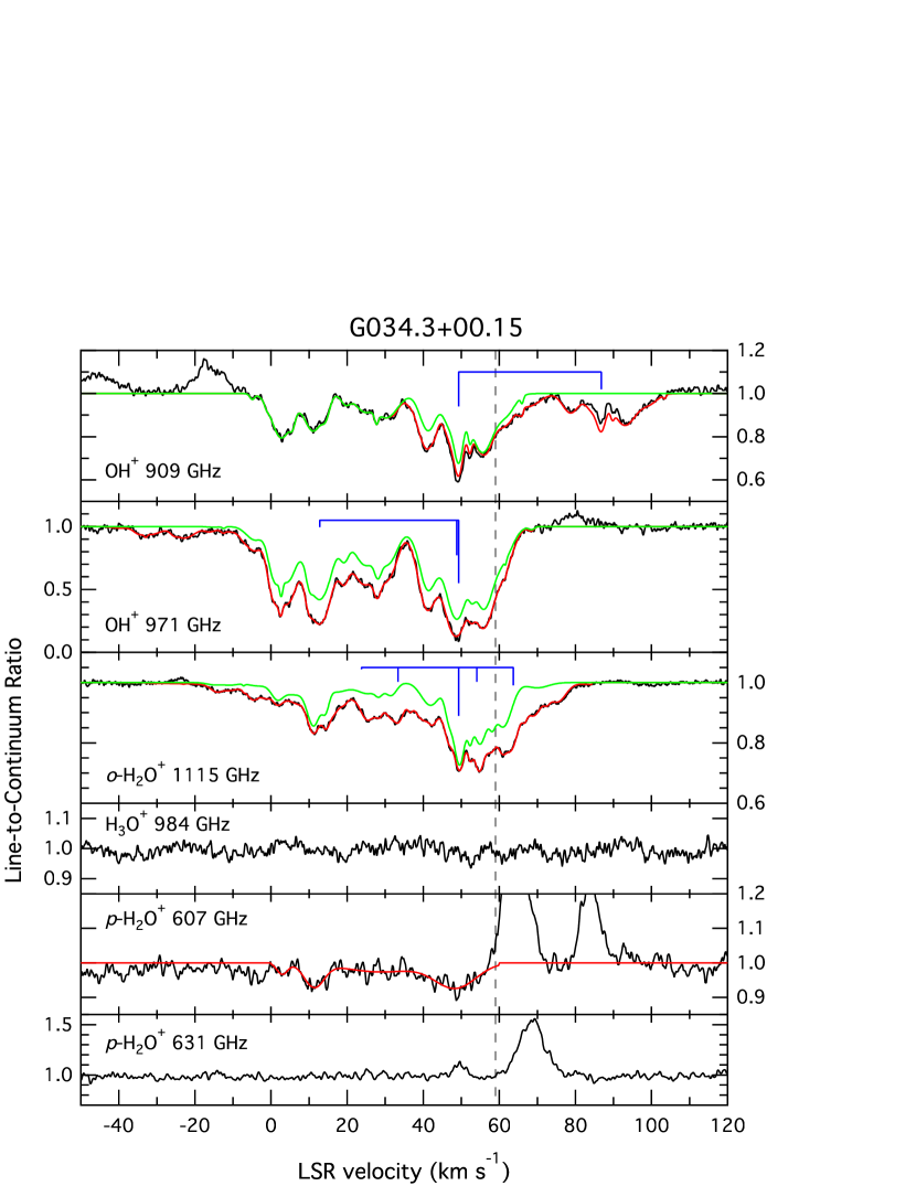
Figure 10: Same as Figure 2 but for G034.3+00.15.

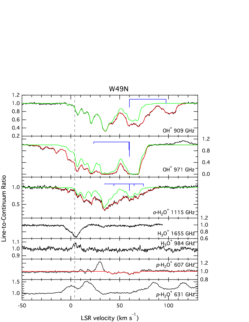
Figure 11: Same as Figure 2 but for W49N.

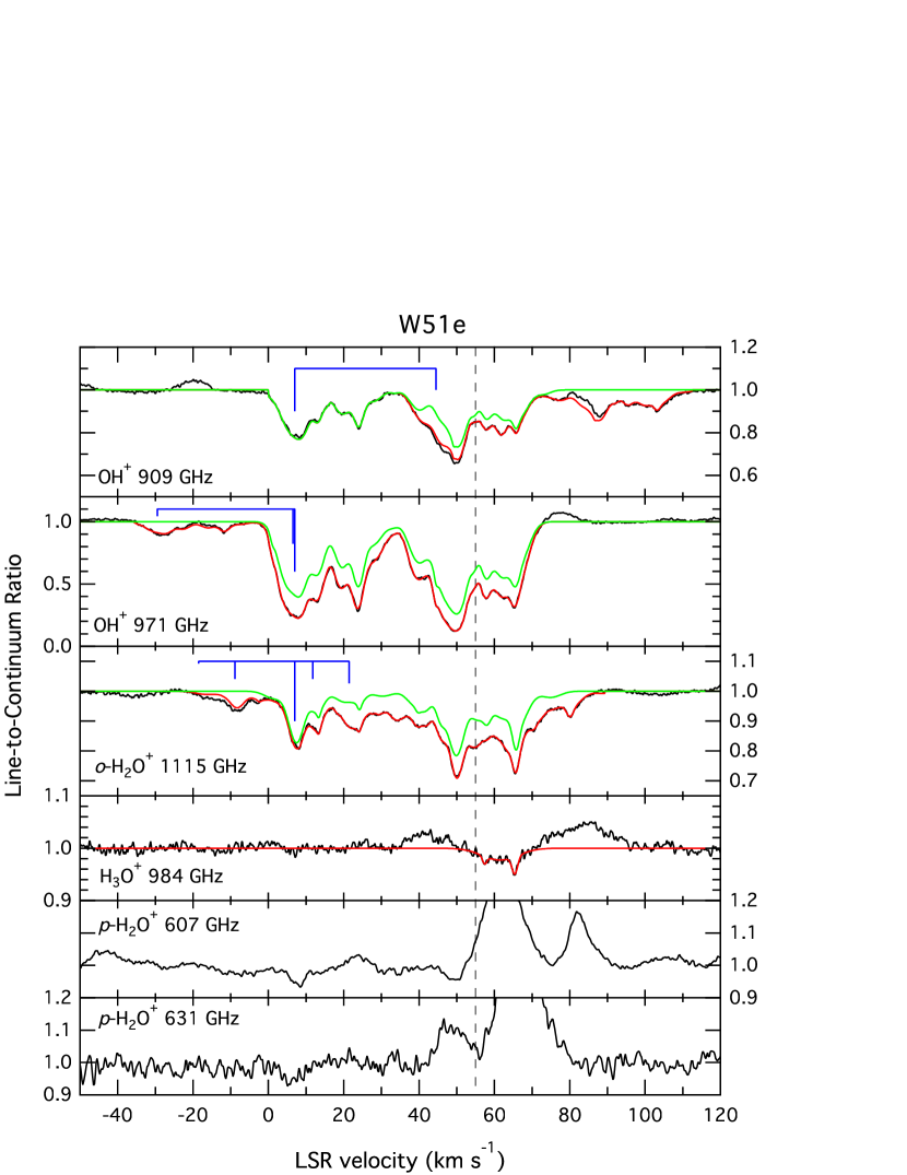
Figure 12: Same as Figure 2 but for W51e.

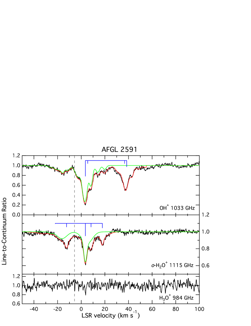
Figure 13: Same as Figure 2 but for AFGL 2591.

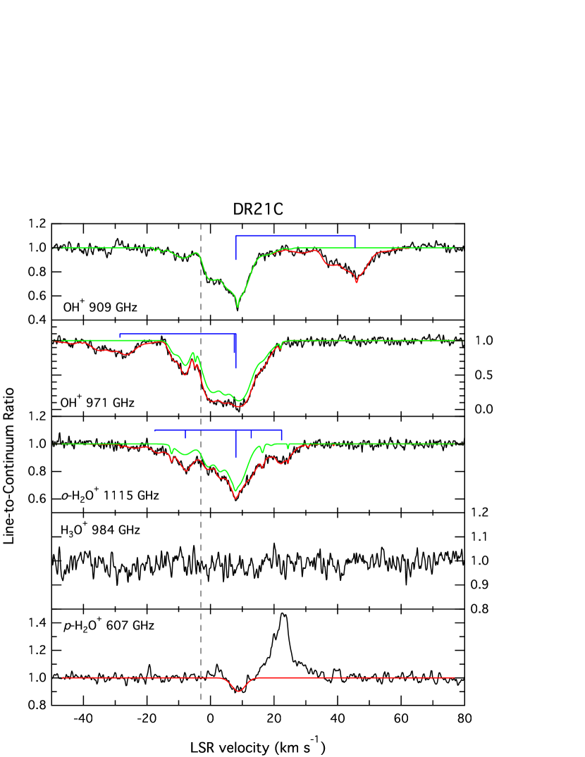
Figure 14: Same as Figure 2 but for DR21C.

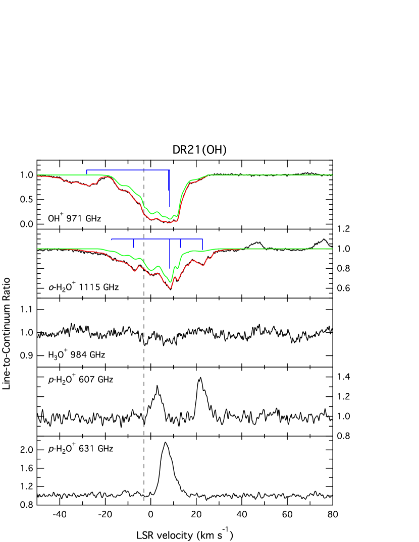
Figure 15: Same as Figure 2 but for DR21(OH).

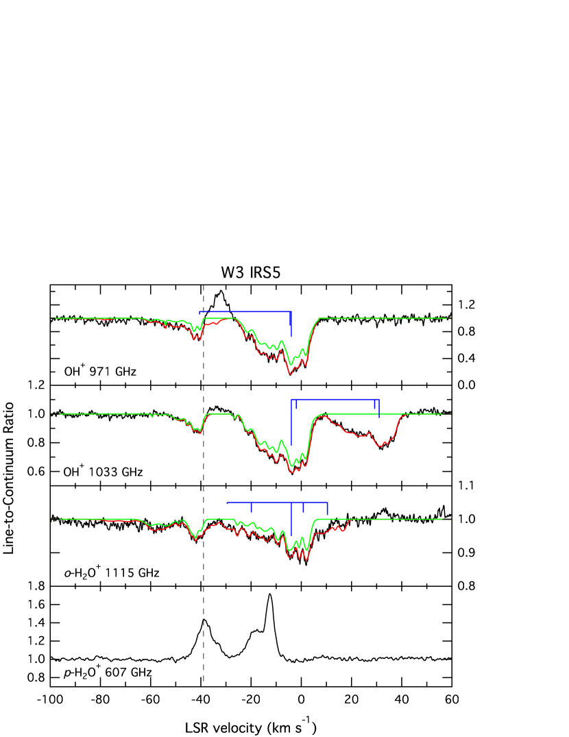
Figure 17: Same as Figure 2 but for W3 IRS5.

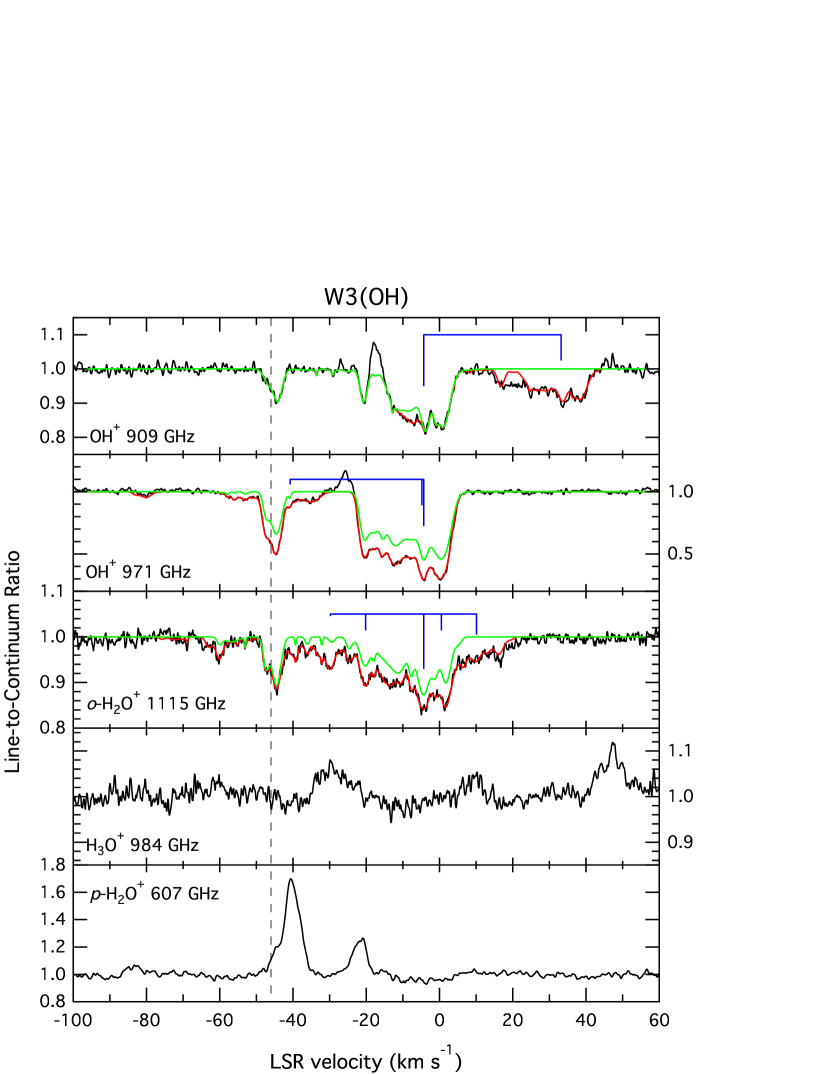
Figure 18: Same as Figure 2 but for W3(OH).

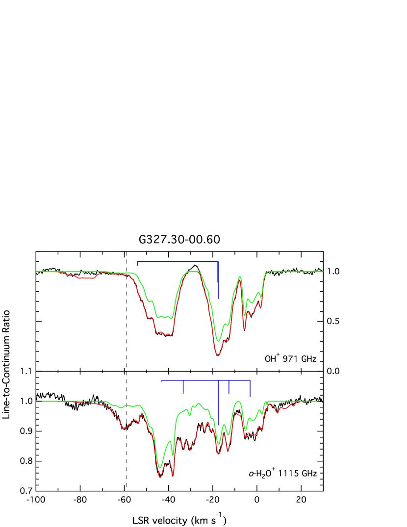
Figure 19: Same as Figure 2 but for G327.30$-$00.60.

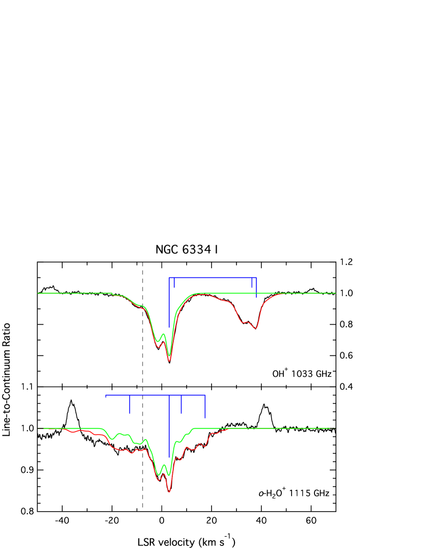
Figure 20: Same as Figure 2 but for NGC 6334 I.

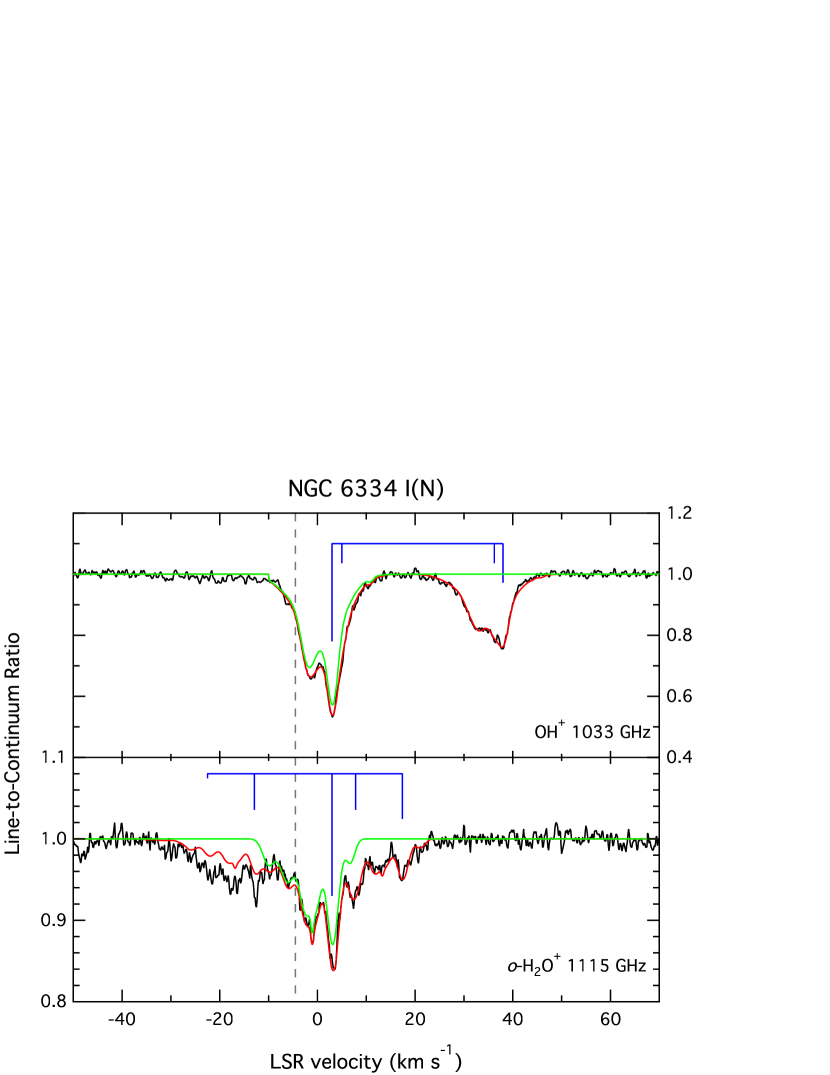
Figure 21: Same as Figure 2 but for NGC 6334 I(N).

The basic fitting procedure used in our analysis has been described previously by Neufeld et al. (2010), but due to some differences we briefly review it here. Absorption features are assumed to result from the combination of multiple components with Gaussian opacity profiles. Each component is defined by a centroid velocity, velocity full-width at half-maximum, and maximum optical depth which act as variables in the fitting process. For transitions with hyperfine structure each component consists of multiple Gaussians in opacity. The strongest hyperfine feature is defined as above, and the other hyperfine features are forced to have the same velocity width, with fixed relative intensities and fixed velocity separations—with respect to the strongest feature—defined by transition frequencies, statistical weights, and spontaneous emission coefficients. Some number of velocity components (between 2 and 20 depending on the complexity of the absorption profile) is initially chosen, and the sum of those components is used to fit the absorption profile. The number of components is then revised as needed to produce a reasonable fit to the spectra. These fits are shown as the red curves in Figures 2–3 and 6–21. To determine the actual distribution of molecules in velocity space when considering a transition with hyperfine splitting, we examine the portion of the fit caused only by the strongest hyperfine feature, as shown by the green curves in Figures 2–21).

3.3 Column Density

From the above fitting procedure we determine the optical depth and differential column density ($dN/dv$) as functions of LSR velocity along a line of sight. The column density in any velocity range can then be determined by integrating $dN/dv$ over that range. Using the OH⁺ and $o$-H₂O⁺ absorption profiles (green curves) we select velocity intervals that correspond to what appear to be separate absorption components, and integrate $dN/dv$ over those intervals. Column densities determined from this analysis for all species are reported in Tables 4 and 5. In all cloud components we assume nearly all molecules are in the ground rotational state for the purpose of determining the total column density of OH⁺ and H₂O⁺ from our observations. Gas densities in diffuse clouds are sufficiently low that collisional excitation is unimportant, and spontaneous radiative decay rates for the studied transitions are large (see Table 1), so the excitation temperature is very likely controlled by the cosmic microwave background radiation (i.e., $T_{ex}\sim 2.7$ K). The assumption that nearly all OH⁺ and H₂O⁺ molecules are in the ground rotational state is thus justified in the diffuse ISM, although in components where the molecules reside in gas that is part of the envelope surrounding the H ii regions used as background sources this may no longer be the case. For H₃O⁺, most of our observations do not probe the lowest lying state, nor is the above assumption valid, so we only report state-specific column densities. In cases where multiple transitions of a given species are observed, the column densities determined from individual transitions are weighted by $1/\sigma^{2}$ (i.e., inverse of the square of the standard deviation presented as uncertainty in Table 4) when determining the average column density for that species (e.g., OH⁺ toward G029.96$-$00.02). If multiple transitions of a species are observed and one transition is saturated (e.g., OH⁺ toward W31C and W49N), only the unsaturated transition is used to determine the column density. When $p$-H₂O⁺ is not detected, an ortho-to-para ratio (OPR) of 3 is assumed in determining $N({\rm H_{2}O^{+}})$ from $N(o$-${\rm H_{2}O^{+}})$. Only for the Sgr B2 sight lines is a different analysis used, where absorption features caused by all transitions of a given species (e.g., 909 GHz, 971 GHz, and 1033 GHz for OH⁺; 1115 GHz and 1139 GHz for $o$-H₂O⁺) are fit simultaneously to determine $dN/dv$ (Schilke et al., 2013).

3.4 Molecular Hydrogen Fraction

A steady-state analysis of the H₂O⁺ abundance governed by reactions (4), (6), and (7) gives the equation

$$n({\rm OH}^{+})n({\rm H}_{2})k_{4}=n({\rm H_{2}O}^{+})[n({\rm H}_{2})k_{6}+n(e)k_{7}],$$ (11)

where $k_{i}$ is the rate coefficient for reaction $i$ within this paper. Through substitutions and rearrangement as shown in Indriolo et al. (2012) this is solved for the molecular hydrogen fraction,

$$f_{\rm H_{2}}=\frac{2x_{e}k_{7}/k_{4}}{N({\rm OH^{+}})/N({\rm H_{2}O^{+}})-k_{6}/k_{4}}.$$ (12)

This assumes constant densities (for the conversion from number density to column density) and constant temperature ($k_{7}$ is temperature dependent) over the region probed. In determining $f_{\rm H_{2}}$ we take $x_{e}=1.5\times 10^{-4}$ (assuming $x_{e}=x({\rm C}^{+})$; Cardelli et al., 1996; Sofia et al., 2004) and $T=100$ K (typical value of the H i spin temperature) in computing the various reaction rate coefficients. Resulting values are presented in Table 5.

3.5 Cosmic-Ray Ionization Rate

A similar analysis of steady-state chemistry for OH⁺ gives

$$\epsilon\zeta_{\rm H}n({\rm H})=n({\rm OH}^{+})[n({\rm H}_{2})k_{4}+n(e)k_{5}].$$ (13)

This equation accounts for the dominant reaction partners by which OH⁺ is destroyed (i.e., H₂ and electrons), but not every instance of hydrogen ionization results in the formation of OH⁺ due to the backward version of reaction (2) and the neutralization of protons on dust grains and PAHs (Wolfire et al., 2003; Liszt, 2003; Hollenbach et al., 2012). To accommodate this fact, we follow Neufeld et al. (2010) in introducing the efficiency factor, $\epsilon$, on the left-hand side of equation (13). Given the same assumptions as above, substitution and rearrangement leads to

$$\epsilon\zeta_{\rm H}=\frac{N({\rm OH}^{+})}{N({\rm H})}n_{\rm H}\left[\frac{f_{\rm H_{2}}}{2}k_{4}+x_{e}k_{5}\right],$$ (14)

and the substitution of equation (12) for $f_{\rm H_{2}}$ to

$$\epsilon\zeta_{\rm H}=\frac{N({\rm OH}^{+})}{N({\rm H})}n_{\rm H}x_{e}\left[\frac{k_{7}}{N({\rm OH^{+}})/N({\rm H_{2}O^{+}})-k_{6}/k_{4}}+k_{5}\right].$$ (15)

In addition to the column densities of OH⁺ and H₂O⁺, this analysis also requires the column density of atomic hydrogen, $N({\rm H})$, and values are reported in Table 5. In several of our target sight lines $N({\rm H})$ is determined from 21 cm absorption observations analyzed by Winkel et al. 2015 (in prep), and in the remainder we have used H i spectra reported in various works (see Table 5 description for references). The number density of hydrogen nuclei is also needed in calculating the ionization rate, and we adopt $n_{\rm H}=35$ cm^-3 following the reasoning in Indriolo et al. (2012). This value arises from assuming that the diffuse atomic outer layers of a cloud with $T=100$ K are in pressure balance with the diffuse molecular interior with $T=70$ K and $n_{\rm H}=100$ cm^-3, and it is in very good agreement with the mean thermal pressure ($\log(P/k)=3.58)$ inferred from fine-structure excitation of C i in diffuse clouds (Jenkins & Tripp, 2011). Still, the determination of interstellar densities is highly uncertain, and we discuss the effects this may have on our analysis below.

Observed column densities of OH⁺, H₂O⁺, and H are then used in concert with rate coefficients and adopted values of $T$, $x_{e}$, and $n_{\rm H}$ to calculate $\epsilon\zeta_{\rm H}$ in each cloud component. To convert $\epsilon\zeta_{\rm H}$ to the cosmic-ray ionization rate the efficiency factor must be known, and we adopt $\epsilon=0.07$ as found during our previous study of the W51e sight line where H${}_{3}^{+}$ observations were used to independently determine the ionization rate and calibrate $\epsilon$ (Indriolo et al., 2012). The value of $\epsilon=0.07\pm 0.04$ presented in Indriolo et al. (2012) is the only observational determination of the efficiency factor, although it has also been computed as part of chemical models studying OH⁺, H₂O⁺, and H₃O⁺ presented by Hollenbach et al. (2012). Those authors find $0.05\lesssim\epsilon\lesssim 0.2$, with the value changing for different densities, ionization rates, depth into a cloud, etc. While our single observational determination of $\epsilon$ falls within the range based on chemical modeling, there is clearly still large uncertainty, and we discuss below the effects that variations in $\epsilon$ have on our analysis. Assuming $\epsilon=0.07$ we calculate the cosmic-ray ionization rate of atomic hydrogen, and values of $\zeta_{\rm H}$ are presented in Table 5.

3.6 Uncertainties in $T$, $x_{e}$, $n_{\rm H}$, and $\epsilon$

During our analysis we have made various assumptions regarding certain variables, namely that $x_{e}=1.5\times 10^{-4}$, $n_{\rm H}=35$ cm^-3, $T=100$ K, and $\epsilon=0.07$ in all cloud components. Here we discuss the uncertainties associated with these parameters.

Temperature (specifically gas kinetic temperature) can affect the rates at which certain chemical reactions occur. The hydrogen abstraction reactions relevant to our analysis (3, 4, and 6) are temperature independent, while dissociative recombination with electrons (reactions 5 and 7) is only weakly dependent on temperature ($k\propto T^{-0.5}$). Inferred temperatures for diffuse molecular clouds do not vary widely ($T\approx 60$–120 K), and we are observing species primarily in the warmer outer regions of these clouds, so uncertainties in $T$ should not significantly affect our results.

The electron fraction is frequently approximated by the C⁺ fractional abundance in diffuse clouds where singly ionized carbon is responsible for the majority of free electrons. This has been found to be about $1.5\times 10^{-4}$ with moderate variance across observed sight lines that probe gas within about 1 kpc of the Sun (Cardelli et al., 1996; Sofia et al., 2004). Metallicities tend to increase at smaller Galactocentric radii (Rolleston et al., 2000), and a typical assumed gradient in carbon abundance results in a factor of 2–3 increase in $x({\rm C})$ at $R_{\rm gal}=3$ kpc (e.g., Wolfire et al., 2003; Pineda et al., 2013; Langer et al., 2014). It is not clear how exactly $x_{e}$ changes with Galactocentric radius, but it is reasonable to assume variations of about a factor of 3 with respect to the adopted value across our sample due to variations in the carbon abundance.

While the contribution to the electron abundance from ionized species other than C⁺ (e.g., Si⁺, S⁺) is generally negligible in diffuse gas, as $\zeta_{\rm H}$ increases the H⁺ abundance can become comparable to or exceed that of C⁺. A prescription for calculating the steady-state value of $x_{e}$ as a function of $\zeta_{\rm H}$ in purely atomic gas is given by Draine (2011), and includes the effects of grain-assisted recombination (Weingartner & Draine, 2001). The resulting electron fraction is dependent on input parameters such as temperature, density, and interstellar radiation field, and for our assumed density $x_{e}$ is relatively constant for $\zeta_{\rm H}\lesssim 10^{-16}$ s^-1, and increases roughly as $\sqrt{\zeta_{\rm H}}$ for larger ionization rates. In this regime, the approximation in equations (14) and (15) that $x_{e}$ is independent of $\zeta_{\rm H}$ begins to break down, and $N({\rm OH}^{+})$ no longer increases linearly with $\zeta_{\rm H}$ (similar to findings for H${}_{3}^{+}$; Liszt, 2007; Goto et al., 2008). In components where we find high ionization rates, $x_{e}$ may in fact be significantly larger than we have assumed (up to a factor of about 20 for $\zeta_{\rm H}\sim 10^{-14}$ s^-1), which would in turn give even larger ionization rates and larger molecular hydrogen fractions than we have reported. Still, given the relationship between $x_{e}$ and $\zeta_{\rm H}$, the values we report remain valid lower limits.

Interstellar gas densities are difficult to constrain and typically have large uncertainties. Estimates of $n_{\rm H}$ are often made using the relative populations in excited states of atoms and molecules. A recent analysis of CO observations gives densities in the range $n_{\rm H}\approx 20$–200 cm^-3 (Goldsmith, 2013), while C₂ observations result in $n_{\rm H}\approx 100$–400 cm^-3 (Sonnentrucker et al., 2007) for diffuse molecular clouds. Excitation of the fine-structure levels of O i has been used to find $n_{\rm H}\approx 5$–25 cm^-3 in diffuse gas (Sonnentrucker et al., 2002, 2003), while excitation of C i has been used to determine thermal pressures that are consistent with $n_{\rm H}\approx 10$–100 cm^-3 (Jenkins & Tripp, 2001, 2011). Observations of C⁺ in many of the same sight lines studied herein are used to infer $n_{\rm H}\approx 40$–100 cm^-3 (Gerin et al., 2014). Clearly, there is large variance among inferred densities for diffuse clouds, although much of this may be due to the specific region probed (i.e., molecular interior versus atomic exterior). If we take the extreme values given above as limits, our adopted value of $n_{\rm H}\approx 35$ cm^-3 can vary up or down by roughly a factor of 10 between different components. However, given the density estimates from Gerin et al. (2014) and pressures inferred by Jenkins & Tripp (2011), it seems likely that this uncertainty is more commonly only a factor of 3 or so in the diffuse foreground gas along our targeted sight lines.

The efficiency factor $\epsilon$ (fraction of instances where cosmic-ray ionization of H leads to formation of OH⁺) has only a single constraint via observations ($\epsilon=0.07\pm 0.04$), and a few estimates from chemical models focused on oxygen-bearing species ($0.05\leq\epsilon\leq 0.2)$. This parameter is affected by gas conditions (e.g., $T$, $n_{\rm H}$, relative abundances), and will vary between different clouds. Our best estimate on the uncertainty in $\epsilon$ comes from the chemical models of Hollenbach et al. (2012), so we consider limits of about a factor of 2 below and a factor of 3 above the adopted value of $\epsilon=0.07$.

3.7 Kinematic Distances

In order to explore any correlation that $f_{\rm H_{2}}$ or $\zeta_{\rm H}$ may have with Galactocentric radius we use a kinematic analysis to estimate $R_{gal}$ for the various velocity intervals of absorbing gas along each line of sight. We adopt the functional form of the rotation curve presented by Persic et al. (1996), and use the input parameters recommended by Reid et al. (2014), including a distance to the Galactic center of 8.34 kpc and a rotation speed of 240 km s^-1. This allows us to determine the expected line-of-sight velocity as a function of $R_{gal}$ given the Galactic longitude of each sight line. Within each velocity interval along a sight line we choose a single velocity—usually corresponding to maximum absorption—which is used in determining $R_{gal}$ for that component. From $R_{gal}$ we determine the near and far kinematic distances to each absorption component. In several cases, departures from the expected velocity due to peculiar motions cause this analysis to produce unphysical results. When the resulting Galactocentric radius is smaller than the radius of the tangent point along a line of sight, we set $R_{gal}$ equal to the tangent point radius. When the kinematic distance is larger than the assumed distance of the background source (see Table 2 and Section 4.1) we set the distance equal to that of the background source and correct $R_{gal}$ accordingly. When the kinematic distance is smaller than 0.1 kpc we set it equal to 0.1 kpc (and adjust $R_{gal}$) so that the gas is outside of the local bubble. For most sight lines the kinematic distance ambiguity is solved because the background source is on the near side of the tangent point. In cases where the ambiguity remains (e.g., W49N) both distances are reported. Some of our target sight lines have distance estimates to foreground clouds available in the literature, which we take to be more robust than our own kinematic analysis. For these sight lines (M$-$0.13$-$0.08, M$-$0.02$-$0.07, Sgr B2(M), Sgr B2(N), W31C, W3 IRS5, and W3(OH); see sections describing individual sight lines for references) we adopt previously determined distances. In the case of AFGL 2591, we assume both absorption components are associated with the background source itself. Galactocentric radii and distances for each velocity component are reported in Table 5.

4 DISCUSSION

As described above, spectra for each sight line were divided into velocity intervals roughly corresponding to absorption features for the purpose of analyzing our data. A total of 105 separate components containing OH⁺ absorption are defined in our sample, of which 100 also show $o$-H₂O⁺ absorption. In contrast, H₃O⁺ absorption is only seen in 16 components (12 of which are in the Galactic center), and $p$-H₂O⁺ absorption in 11 components (4 of which are in the Galactic center). In many cases though, potential for detection of the $p$-H₂O⁺ 607 GHz line is impeded by emission from the $J=7$–6 transition of H¹³CO⁺ (607.1747 GHz) and the $J_{K_{a},K_{c}}=12_{2,10}$–11_1,10 transition of CH₃OH (607.2158 GHz). Similarly, the 631 GHz transition of $p$-H₂O⁺ is often obscured by emission from the $J_{K_{a},K_{c}}=9_{1,9}$–8_1,8 transition of H₂CO (631.7028 GHz). The rest frequency of the H₃O⁺ 1655 GHz transition is only 34 MHz below (6 km s^-1 redshift) that of the 2_1,2–1_0,1 transition of H${}_{2}^{18}$O, making a confirmed detection difficult. Only in two sight lines (W31C and W49N) do we present the 1655 GHz spectra, as in all others where the transition was covered we are confident the absorption signals are due to H${}_{2}^{18}$O (identification aided by absorption profiles of the 1_1,1–0_0,0 transition of H${}_{2}^{18}$O presented in van der Tak et al., 2013b). A more detailed description of our findings in each line of sight follows.

4.1 Line of Sight Properties

4.1.1 M$-$0.13$-$0.08 and M$-$0.02$-$0.07

Two well known molecular clouds in the Galactic center region are M$-$0.13$-$0.08 and M$-$0.02$-$0.07, also commonly referred to as the Sgr A +20 km s^-1 and Sgr A +50 km s^-1 clouds due to their respective radial velocities. Both are within 10 pc of the Galactic center (Ferrière, 2012), which is 8.34$\pm$0.16 kpc away from the Sun (Reid et al., 2014), and are separated by a projected distance of 15.6 pc. Each cloud has associated compact H ii regions—source SgrA–G from Ho et al. (1985) in the case of M$-$0.13$-$0.08, and SgrA–A, SgrA–B, SgrA–C, and SgrA–D (also referred to as the G$-$0.02$-$0.07 complex) in the case of M$-$0.02$-$0.07 (Ekers et al., 1983; Mills et al., 2011)—but it is cool dust that serves as the background continuum sources for these sight lines.

M$-$0.13$-$0.08 shows OH⁺ absorption across the entire velocity range from $-$210 km s^-1 to 30 km s^-1 (Figure 2). Absorption at $v_{\rm LSR}\lesssim-60$ km s^-1 is thought to be due entirely to gas in the central molecular zone (CMZ) within the Galactic center region (Sonnentrucker et al., 2013), while at $v_{\rm LSR}\gtrsim-60$ km s^-1 there is some combination of foreground spiral arms that absorb at distinct velocities and gas in the CMZ. We attribute absorption at $-50$ km s${}^{-1}\leq v_{\rm LSR}\leq-40$ km s^-1 to the 3 kpc spiral arm (Dame & Thaddeus, 2008), and at $-40$ km s${}^{-1}\leq v_{\rm LSR}\leq-15$ km s^-1 to the 4.5 kpc spiral arm (Menon & Ciotti, 1970), although both intervals are likely contaminated by gas in the Galactic center as well. Absorption from $-$15 km s^-1 to 30 km s^-1 is due to some combination of local gas and the CMZ, including the cloud in which the continuum source is embedded (i.e., the +20 km s^-1 cloud). The $o$-H₂O⁺ spectrum follows a similar pattern, but with weaker absorption in many components. H₃O⁺ absorption is only seen in a narrow component at 12 km s^-1, coming from the molecular cloud itself.

Similarly, M$-$0.02$-$0.07 shows OH⁺ and $o$-H₂O⁺ absorption from $-$210 km s^-1 to 70 km s^-1 (Figure 3). We assume roughly the same breakdown between CMZ and foreground gas, with the 3 kpc spiral arm at $-61$ km s${}^{-1}\leq v_{\rm LSR}\leq-47$ km s^-1, the 4.5 kpc spiral arm at $-47$ km s${}^{-1}\leq v_{\rm LSR}\leq-13$ km s^-1, and the CMZ at $v_{\rm LSR}\leq-61$ km s^-1 and $v_{\rm LSR}\geq-13$ km s^-1. The background molecular cloud (Sgr A +50 km s^-1) is responsible for absorption between 20 km s^-1 and 70 km s^-1. Again, the background source is the only component that shows substantial H₃O⁺ absorption, although there may also be a weak feature at $-140$ km s^-1. Both the 607 GHz and 631 GHz transitions of $p$-H₂O⁺ were also targeted toward M$-$0.02$-$0.07, and, despite high noise levels, we consider the features at $-140$ km s^-1 that coincide with the strongest $o$-H₂O⁺ absorption to be detections. Values of $N(p{\rm-H_{2}O^{+}})$ derived from both transitions are in agreement.

It must be noted that for both sight lines blending of absorption from foreground spiral arms and from the CMZ complicates our analysis. We have attributed absorption in select velocity intervals entirely to foreground clouds following previous studies of molecular absorption toward the Galactic center (e.g., Monje et al., 2011; Sonnentrucker et al., 2013; Schilke et al., 2010, 2014), but other studies have shown that the entire velocity range under consideration also contains absorption from gas in the CMZ (e.g., Oka et al., 2005; Geballe & Oka, 2010; Goto et al., 2011, 2014). Results inferred from absorption in these velocity ranges—i.e., those assigned to the 3 kpc and 4.5 kpc spiral arms—should be viewed with caution. The same is true for select velocity intervals in the Sgr B2 sight lines discussed below.

4.1.2 Sgr B2(M) and Sgr B2(N)

Sgr B2 is a giant molecular cloud within the Galactic center region that contains multiple cores—including Sgr B2(M) and Sgr B2(N)—where prolific star formation is occurring. Different studies place Sgr B2 in front of (Reid et al., 2009) or behind (Molinari et al., 2011) Sgr A*, but always within $\sim 150$ pc, and we adopt $d=8.34$ kpc, as the precise location is not vital to our study. At this distance the projected separation between Sgr B2 and Sgr A* is about 100 pc, and the projected separation between the Sgr B2(M) and Sgr B2(N) cores is 1.8 pc.

Spectra of OH⁺, H₂O⁺, and H₃O⁺ toward Sgr B2(M) and Sgr B2(N) are largely similar (Figures 4 and 5) with strong absorption extending from about $-120$ km s^-1 to 40 km s^-1. Absorption across this entire velocity range is likely caused by gas within the Galactic center and foreground spiral arms that contribute at specific velocities. The lack of sharp, well-defined features makes it difficult to attribute absorption to any particular spiral arm, but we assume that absorption in the $-60$ km s${}^{-1}\lesssim v_{\rm LSR}\lesssim-30$ km s^-1 interval arises in the 3 kpc arm, and in the $-30$ km s${}^{-1}\lesssim v_{\rm LSR}\lesssim-5$ km s^-1 interval in the 4.5 kpc arm, with the caveat that there is likely considerable contamination from gas within the Galactic center as well. Systemic velocities of the background sources differ slightly, about 63 km s^-1 for Sgr B2(M) and 66 km s^-1 for Sgr B2(N), and both sources show absorption, but Sgr B2(N) has an additional absorption component near 80 km s^-1 seen only in H₃O⁺. The Sgr B2 sight lines are unique in our survey in that H₃O⁺ absorption is detected in all velocity components. While we only list column densities in the 1${}_{0}^{+}$ state, a much more thorough analysis utilizing transitions out of 11 levels of H₃O⁺ in these sight lines (beyond the scope of this paper) has been carried out by Lis et al. (2014). Our reported values for $N(1_{0}^{+})$ are in good agreement with theirs.

Although several spectra of both ortho and para H₂O⁺ toward Sgr B2(M) have been presented and analyzed in previous studies (Ossenkopf et al., 2010; Schilke et al., 2010, 2013), we reproduce the 1115 GHz and 1139 GHz absorption lines here to facilitate comparison with OH⁺. Both the 971 GHz and 1033 GHz lines of OH⁺ are saturated, and knowledge of the velocity structure is almost entirely dependent on the 909 GHz transition. Still, the OH⁺ and $o$-H₂O⁺ profiles are nearly identical in velocity structure for both Sgr B2(M) and Sgr B2(N). These sight lines are also unique in that $p$-H₂O⁺ is detected in all velocity components as shown by Schilke et al. (2013), and where available we use column densities determined from that study in computing the OPR shown in Table 4, as well as total $N({\rm H_{2}O}^{+})$.

4.1.3 W28A

The ultracompact H ii region W28A (also known as G005.89$-$00.39) is a site of active star formation located 1.28 kpc away from the Sun (Motogi et al., 2011) that lies about 40′ south of the W28 supernova remnant, although it is unclear if the two sources are physically related or a chance projection. Molecular line observations give a systemic velocity of 9 km s^-1 for W28A (Harvey & Forveille, 1988; Nicholas et al., 2011). OH⁺ shows three distinct absorption components at about 7 km s^-1, 13 km s^-1, and 23 km s^-1 (Figure 6). The first two of these are detected in $o$-H₂O⁺, but the component at 23 km s^-1 is clearly absent. In the two components where both ions are detected, we find molecular hydrogen fractions of about 0.085, above average in our sample. Neither $p$-H₂O⁺ nor H₃O⁺ is detected in absorption toward W28A, but it is possible that the weak emission at 9 km s^-1 in the H₃O⁺ spectrum is arising in the background source itself.

4.1.4 W31C

Also commonly referred to as G010.62$-$00.38, W31C is an H ii region within the W31 complex, and has a systemic velocity of about $-4$ km s^-1 (Godard et al., 2010; Gerin et al., 2010a). The H ii region has a large peculiar motion with respect to the Galaxy’s rotation curve, and is 4.95 kpc away from the Sun as determined by H₂O maser observations (Sanna et al., 2014). A detailed picture of the velocity components along the line of sight is given by Corbel & Eikenberry (2004), and we use their distance estimates rather than simple kinematic rotation curve estimates in our analysis.

OH⁺ shows absorption from about $-10$ km s^-1 to 50 km s^-1, and although the 971 GHz transition is saturated in multiple components the velocity profile of the 909 GHz transition is rather well matched by that of $o$-H₂O⁺ (Figure 7). The strongest OH⁺ and $o$-H₂O⁺ absorption is in a narrow component centered at about 40 km s^-1, which also shows absorption from H₃O⁺ in both the 1655 GHz and 984 GHz lines (full analysis in Lis et al., 2014) and $p$-H₂O⁺ in the 607 GHz line. A feature in the $p$-H₂O⁺ 631 GHz spectrum may also be related to this narrow component, but given the noise level we treat it as a non-detection. A broad, weak feature in the H₃O⁺ 984 GHz spectrum from about 13 km s^-1 to 30 km s^-1 is also thought to be caused by H₃O⁺. Absorption near $-$6 km s^-1 in the 1655 GHz H₃O⁺ spectrum, however, is likely caused entirely by the 2_1,2–1_0,1 transition of H${}_{2}^{18}$O mentioned above.

All species studied here (OH⁺, $o$-H₂O⁺, $p$-H₂O⁺, and H₃O⁺) were previously reported in absorption by Gerin et al. (2010b). A direct comparison of derived column densities is complicated by the different velocity intervals chosen. An analysis of the OPR of H₂O⁺ toward W31C was performed by Gerin et al. (2013), and our results (see Table 4) are in rough agreement with their findings despite the use of different velocity intervals. Lis et al. (2014) also performed a multi-level analysis of H₃O⁺ (using 6 transitions) in this sight line, and our reported column densities agree within uncertainties.

4.1.5 W33A

Trigonometric parallax observations of water masers in the W33 star forming complex put the region—including the massive young stellar object W33A—at a distance of 2.4 kpc (Immer et al., 2013). W33A (also identified as the H ii region G012.90$-$00.26) has a systemic velocity of about 37 km s^-1 as measured from various emission lines (e.g. van der Tak et al., 2000; Wienen et al., 2012; San José-García et al., 2013). OH⁺ shows four separate absorption features from $-$4 km s^-1 to 16 km s^-1, 20 km s^-1 to 25 km s^-1, 25 km s^-1 to 36 km s^-1 and 36 km s^-1 to 45 km s^-1 (Figure 8), all of which are also detected in $o$-H₂O⁺ absorption. In all of these components we find $0.07\leq f_{\rm H_{2}}\leq 0.09$, above the average value for foreground gas. Neither $p$-H₂O⁺ nor H₃O⁺ are detected along this sight line.

4.1.6 G029.96$-$00.02

The ultracompact H ii region G029.96$-$00.02 is 5.26 kpc away from the Sun as determined via maser trigonometric parallax (Zhang et al., 2014). It has a systemic velocity of about 98 km s^-1, very near the tangent velocity, and absorption occurs nearly continuously from there down to 0 km s^-1 in several distinct velocity components, as can be seen in our OH⁺ and $o$-H₂O⁺ spectra (Figure 9). Neither H₃O⁺ nor $p$-H₂O⁺ are conclusively detected, although there is a weak (2$\sigma$) feature in the 607 GHz spectrum at 71 km s^-1 (where the strongest OH⁺ and $o$-H₂O⁺ absorption occurs) that may be due to $p$-H₂O⁺. Interestingly, three of the components along this sight line (those centered at 53 km s^-1, 83 km s^-1, and 92 km s^-1) have the three lowest values of the cosmic-ray ionization rate inferred by our analysis.

4.1.7 G034.3+00.15

G034.3$+$00.15 shows molecular emission at about 59 km s^-1 (HCO⁺ from Godard et al., 2010), and the compact H ii region is about 3.8 kpc away from the Sun as determined by a kinematic analysis (Fish et al., 2003). Absorption between about 44 km s^-1 and 70 km s^-1 is likely associated with the background source and molecular cloud itself, while absorption at lower velocities is due to foreground material. The OH⁺ and $o$-H₂O⁺ spectra (Figure 10) show relatively similar absorption profiles, and H₃O⁺ is not detected. The $p$-H₂O⁺ 607 GHz spectrum shows weak absorption at 8–16 km s^-1 and 40–55 km s^-1, both ranges that match the strongest OH⁺ features. No absorption is detected from the $p$-H₂O⁺ 631 GHz transition.

4.1.8 W49N

W49N contains several ultracompact H ii regions, and at 11.11 kpc away (determined from H₂O maser observations of Zhang et al., 2013) this is the most distant source we have observed. Molecular emission peaks near 0–8 km s^-1 for HCO⁺ (Godard et al., 2010) and CH (Gerin et al., 2010a), marking the systemic velocity for W49N, and these emission features tend to be broad with FWHM$\sim$10 km s^-1. Absorption extends up to about 80 km s^-1 going from the background source to the tangent point (Figure 11), and then sweeps back down to 0 km s^-1 going from the tangent point to the Sun (Fish et al., 2003). This means that a rotation curve analysis of the gas velocities will result in both a near and far estimate, making distance determinations highly uncertain. Because unassociated clouds will be absorbing at the same velocities the determination of abundance ratios, $f_{\rm H_{2}}$, and $\zeta_{\rm H}$ will also be highly uncertain, and results from this sight line should be viewed with caution.

OH⁺ and $o$-H₂O⁺ were previously analyzed toward W49N by Neufeld et al. (2010), although only the 971 GHz OH⁺ data were available at that time. Column densities based on both the 909 GHz and 971 GHz transitions are similar to those reported by Neufeld et al. (2010). The 607 GHz transition of $p$-H₂O⁺ is also seen in absorption from about 35 km s^-1 to 70 km s^-1, and has previously been analyzed by Gerin et al. (2013) for the purpose of studying the OPR of H₂O⁺. Although their analysis split the H₂O⁺ absorption into 5 km s^-1 bins, the resulting OPR agree well with those we present in Table 4. There is a hint of absorption from the 631 GHz line of $p$-H₂O⁺ near 35 km s^-1, but interference from a strong emission line due to H₂CO complicates the analysis of this feature. The 984 GHz H₃O⁺ transition may show weak emission at the source velocity, but is not seen in absorption. The 1655 GHz H₃O⁺ transition potentially shows absorption (2$\sigma$ level) at 34 km s^-1 (matches strongest OH⁺ and H₂O⁺ in velocity), but near the systemic velocity there is likely strong blending with H${}_{2}^{18}$O absorption as was the case for W31C.

4.1.9 W51e

The W51 region consists of a massive molecular cloud and several active star forming complexes, and has an inferred distance of 5.41 kpc from H₂O maser observations (Sato et al., 2010). The compact H ii regions W51 e1 and W51 e2 (Mehringer, 1994) were used as background continuum sources for our observations, and show molecular emission features centered at 55 km s^-1 (Ho & Young, 1996; Sollins et al., 2004). Narrow absorption at 70 km s^-1 is caused by a cold dense clump (Mookerjea et al., 2014), while a more broadly distributed foreground cloud absorbs at 62–70 km s^-1, and gas between about 44 km s^-1 and 62 km s^-1 is associated with the giant molecular cloud itself (Kang et al., 2010). Gas absorbing at lower velocities (e.g., 7 km s^-1 and 24 km s^-1) is well in the foreground, and likely more diffuse (Carpenter & Sanders, 1998; Sonnentrucker et al., 2010).

Observations of $o$-H₂O⁺ from the WISH (Water In Star-Forming regions with Herschel) program were previously presented by Wyrowski et al. (2010b), and observations of $o$-H₂O⁺ and OH⁺ from the PRISMAS program by Indriolo et al. (2012). Our column densities are in good agreement with those reported in the above studies, but should supersede previous values as the $o$-H₂O⁺ spectra we present utilize a combination of WISH, PRISMAS, and OT1_dneufeld_1 data, and have significant improvement in S/N (Figure 12). Analyses of OH⁺ from both the 909 GHz and 971 GHz transitions are in good agreement, and differences in derived column densities can be attributed to interference from a weak emission line due to the 5${}_{5,1}^{+}$–6${}_{4,2}^{+}$ and 5${}_{5,0}^{-}$–6${}_{4,3}^{-}$ transitions of CH₃OH at 909.0744 GHz that can be seen in the 909 GHz spectrum as a poor fit near 85 km s^-1. This causes an underestimate of $N({\rm OH}^{+})$ in the $42~{}{\rm km~{}s}^{-1}\leq v_{\rm LSR}\leq 55~{}{\rm km~{}s}^{-1}$ interval, and overestimate in the $-4~{}{\rm km~{}s}^{-1}\leq v_{\rm LSR}\leq 16~{}{\rm km~{}s}^{-1}$ interval. As a result, only the 971 GHz line is used in determining $N({\rm OH}^{+})$ over these intervals.

The diffuse cloud near 6 km s^-1 shows absorption from the 607 GHz transition of $p$-H₂O⁺ (absorption near 50 km s^-1 is also likely, but interference from a strong emission line of CH₃OH complicates the analysis there). Additionally, the components at 55–75 km s^-1 are two of only four outside the Galactic center in our survey where H₃O⁺ absorption is detected via the 984 GHz transition. The features are very weak, but match exceptionally well in velocity space with absorption peaks in the $o$-H₂O⁺ spectrum and both OH⁺ spectra. This H₃O⁺ absorption denotes gas that has a high molecular fraction and is likely in a dense cloud interior rather than the diffuse outer layers (following the model of Hollenbach et al., 2012), a hypothesis supported by the fact that this velocity component shows the strongest absorption in HF and H₂O along the W51e sight line (Sonnentrucker et al., 2010).

4.1.10 AFGL 2591

AFGL 2591 is a cluster of high mass protostars with a bipolar outflow likely driven by the source associated with 1.3 cm and 3.6 cm continuum emission identified as VLA 3 (Trinidad et al., 2003). The molecular gas associated with the protostars has a velocity of $-5.5$ km s^-1 (van der Tak et al., 1999), and H₂O maser observations give a distance of 3.33 kpc (Rygl et al., 2012). OH⁺ and H₂O⁺ show two components in absorption toward AFGL 2591, at 3 km s^-1 and $-17$ km s^-1, neither of which matches the systemic velocity (Figure 13). The gas at 3 km s^-1 may be associated with a foreground cloud previously reported at 0 km s^-1 in tracers of molecular gas (Emprechtinger et al., 2012; van der Wiel et al., 2013), but this requires a velocity offset between the molecular cloud and the atomic outer layers where the oxygen ions presumably reside. The blueshifted component at $-17$ km s^-1 may be associated with a molecular outflow (Mitchell et al., 1989; van der Tak et al., 1999, 2013b; van der Wiel et al., 2013), a hypothesis that could explain the larger value of $f_{\rm H_{2}}=0.09$ found in this component. Both OH⁺ and H₂O⁺ have previously been studied toward AFGL 2591 (Bruderer et al., 2010; Benz et al., 2013) along with several other light hydrides. The column densities that we derive for the two velocity components are in relatively good agreement with those found by Bruderer et al. (2010), as well as the line of sight column densities reported by Benz et al. (2013). H₃O⁺ absorption is not detected, likely due to the low continuum level signal-to-noise ratio, although emission from the $4_{3}^{+}-3_{3}^{-}$ transition has been observed at the systemic velocity (Benz et al., 2013). A more detailed study of light hydrides in AFGL 2591 is currently underway (Benz et al. 2015, in preparation).

4.1.11 DR21C and DR21(OH)

DR21C and DR21(OH) are compact H ii regions that are parts of the DR21 molecular ridge, a region of massive star formation about 1.5 kpc away from the Sun (determined from H₂O maser observations by Rygl et al., 2012). Systemic velocities for both sources are about $-3$ km s^-1 (van der Tak et al., 2010; Zapata et al., 2012). The sources are separated by 3.1′ on sky, corresponding to a projected separation of 1.3 pc at the adopted distance. The OH⁺ and $o$-H₂O⁺ absorption profiles for DR21C and DR21(OH) are largely similar (Figures 14 and 15). In the OH⁺ spectra there is a shallow absorption wing from about 25 km s^-1 to 15 km s^-1, followed by a rapid increase to maximum absorption near 9 km s^-1. The absorption then gradually decreases until it disappears around $-15$ km s^-1. The most notable difference between the spectra is that toward DR21C there is a local minimum in absorption at $-5$ km s^-1, while for DR21(OH) the absorption decreases monotonically below 0 km s^-1. Spectra of $o$-H₂O⁺ show the same general structure. Differences in the absorption profiles between the two sources only occur near the systemic velocities, suggesting that most of the absorption arises in a common foreground cloud. Indeed, the strongest absorption at 9 km s^-1 matches a foreground cloud observed in CO and HCO⁺ associated with the nearby source W75N (Schneider et al., 2010). Neither the 607 GHz nor the 631 GHz transition of $p$-H₂O⁺ is detected toward DR21(OH), but the 607 GHz line shows absorption toward DR21C, although there is likely interference from emission lines of CH₃OH and H¹³CO⁺. H₃O⁺ is not detected in either sight line. Previous observations of $o$-H₂O⁺ toward DR21C were reported by Ossenkopf et al. (2010), and our resulting column densities are in relatively good agreement. Our inferred column densities for OH⁺ and H₂O⁺ are also in good agreement with those found as part of a more detailed analysis of the DR21C sight line (Chambers et al. 2015, in preparation)

4.1.12 NGC 7538 IRS1

The hyper-compact H ii region NGC 7538 IRS1 is 2.65 kpc distant as determined via trigonometric parallax of CH₃OH masers (Moscadelli et al., 2009) and has a systemic velocity of $-59$ km s^-1 observed in several molecules (Zhu et al., 2013). OH⁺ and $o$-H₂O⁺ show very similar absorption profiles with components at $-50$ km s^-1, $-33$ km s^-1, $-28$ km s^-1, $-7$ km s^-1, and 0 km s^-1, the exception being that the $-$28 km s^-1 component is missing in $o$-H₂O⁺ (Figure 16). Absorption from $-$60 km s^-1 to $-$40 km s^-1 is likely associated with material at the background source, while the other components arise in foreground gas. A detailed analysis of light hydrides in NGC 7538 IRS1 is forthcoming in Benz et al. 2015 (in preparation).

4.1.13 W3 IRS5 and W3(OH)

Both W3(OH) and W3 IRS5 are located in the W3 molecular cloud complex, a site of active star formation within the Galaxy. W3(OH) is an ultracompact H ii region thought to harbor a massive young star, while W3 IRS5 is a protocluster of a few high mass stars. Multi-epoch VLBA observations of water masers toward both sources have been used to determine distances of $2.04\pm 0.07$ kpc (Hachisuka et al., 2006) and $1.83\pm 0.14$ kpc (Imai et al., 2000) for W3(OH) and W3 IRS5, respectively. Molecular line observations show systemic velocities of $-46$ km s^-1 for W3(OH) (Wilson et al., 1991) and $-39$ km s^-1 for W3 IRS5 (Wang et al., 2013). The two sources are 16.6′ apart in the sky, corresponding to a projected separation of about 9.7 pc at the distance of the background sources.

The absorption profiles of OH⁺ and $o$-H₂O⁺ toward W3(OH) and W3 IRS5 are largely similar, with absorption from about 7 km s^-1 to $-27$ km s^-1 (Figures 17 and 18). These features are due to foreground clouds that have previously been observed in H i absorption at about 0 km s^-1 and $-20$ km s^-1, and which are estimated to be at distances of 0.7 kpc and 1.5 kpc, respectively (Normandeau, 1999). Toward W3(OH) the absorption between $-41$ km s^-1 and $-50$ km s^-1 is likely associated with material surrounding the background source itself, and similar for the $-37$ km s^-1 to $-47$ km s^-1 absorption toward W3 IRS5. Neither line of sight shows a conclusive detection of the $p$-H₂O⁺ line at 607 GHz, nor is H₃O⁺ detected toward W3(OH). Emission features in the 909 GHz spectrum toward W3(OH) and in the 971 GHz spectrum toward W3 IRS5 are due to CH₃OH.

Analyses of light hydrides in the W3 IRS5 sight line have been previously reported by Benz et al. (2010, 2013). Column densities that we find for OH⁺ and $o$-H₂O⁺ in the foreground gas are consistent with those reported by Benz et al. (2010), within uncertainties. For the gas associated with the background source, however, our column densities are about half of the values reported in Benz et al. 2015 (in preparation). The difference arises because we assume the entire populations of both species are in the ground state, while Benz et al. 2015 (in preparation) adopt a higher excitation temperature to account for heating by UV radiation, assuming the gas is located in the cavity wall of a protostellar outflow.

4.1.14 G327.3-0.6

G327.3$-$0.6 is a hot core within a region of active star formation, and provides the longest line of sight probing the fourth Galactic quadrant in our study. Molecular emission lines give a systemic velocity of $-$44.5 km s^-1 (San José-García et al., 2013; Leurini et al., 2013), and a distance of 3.3 kpc was determined via a kinematic analysis of H i absorption data (Urquhart et al., 2012). OH⁺ and $o$-H₂O⁺ show similar absorption profiles for the most part (Figure 19). Absorption from $-$31 km s^-1 to $-$55 km s^-1 likely arises within the cloud containing the background source, while features at $v_{\rm LSR}\geq-26$ km s^-1 are caused by foreground material. It is unclear why the expected absorption due to the weakest hyperfine component of the OH⁺ 971 GHz transition fails to match the observed spectrum near $-$75 km s^-1.

4.1.15 NGC 6334 I and NGC 6334 I(N)

The sources NGC 6334 I (a hot molecular core) and NGC 6334 I(N) (a mid-IR quiet high mass protostellar object) are both within the NGC 6334 complex of molecular clouds and H ii regions, located at a distance of 1.35 kpc (Wu et al., 2014). Systemic velocities for the two sources are $-$7.7 km s^-1 and $-$4.5 km s^-1, respectively, and they are separated by 1.9′ on sky, corresponding to projected separation of 0.74 pc at the adopted distance. Absorption profiles of OH⁺ and $o$-H₂O⁺ are nearly identical between the two sight lines with peaks at 3 km s^-1 and $-$2 km s^-1, although NGC 6334 I also shows a weaker component near $-$10 km s^-1 (Figures 20 and 21). None of these components are well-matched to those seen in H₂O (van der Tak et al., 2013b) and HF (Emprechtinger et al., 2012) that have been attributed to protostellar envelopes, outflows, and foreground clouds, further highlighting the different regions traced by such molecules. Given the similarities between the two sight lines though, we can conclude that the absorption features at 3 km s^-1 and $-$2 km s^-1 likely arise in a common foreground cloud. A detailed analysis of light hydrides in the background sources will be presented by Benz et al. 2015 (in preparation). Column densities of OH⁺ and H₂O⁺ toward NGC 6334 I have previously been reported by Zernickel et al. (2012). Our findings for OH⁺ where they adopt an excitation temperature of 2.7 K are in good agreement, but for H₂O⁺ their adopted value of $T_{ex}=24$ K leads to a much larger column density.

4.2 H₂O⁺ ortho-to-para ratio (OPR)

Out of our entire survey, 11 velocity intervals show conclusive detections of the $p$-H₂O⁺ line at 607 GHz, and only 6 of those are above a 3$\sigma$ level. Four of the detections are along Galactic center sight lines, including one toward M$-$0.02$-$0.07 and three toward Sgr B2(M) previously reported by Schilke et al. (2013). These 11 components provide the opportunity to investigate the OPR of H₂O⁺, which is given in Table 4 column 9. In all cases, within uncertainties the OPR is consistent with a value of 3, the ratio expected in the high temperature limit based solely on nuclear spin statistical weights. While it is possible that reactive collisions, temperature, forbidden spontaneous emission (Tanaka et al., 2013), and state-specific formation and destruction can skew the OPR away from 3, observations thus far have not conclusively demonstrated any such deviations in the diffuse ISM (Gerin et al., 2013; Schilke et al., 2013).

4.3 H₃O⁺ Detections

H₃O⁺ is only detected in absorption in 16 components, 12 of which are in sight lines toward the Galactic center. Models of the chemistry surrounding oxygen-bearing ions find that H₃O⁺ will only form in observable abundances in gas that is well shielded from the interstellar radiation field (visual extinction, $A_{V}\gtrsim 3$ mag; Hollenbach et al., 2012). In such regions, the oxygen chemistry is driven by the reaction $\mathrm{O+H_{3}^{+}\rightarrow OH^{+}+H_{2}}$ rather than reaction (3), so abundances are linked to the ionization rate of H₂ instead of H. The small number of H₃O⁺ detections in our sample suggests that most of the components we consider have low $A_{V}$, and are comprised of diffuse gas. This supports the use of diffuse cloud chemistry in our analysis, the link between OH⁺ and the ionization rate of atomic hydrogen, and the assumption that molecules are almost entirely in their respective ground states.

4.4 Molecular hydrogen fraction and OH⁺ to H₂O⁺ ratio

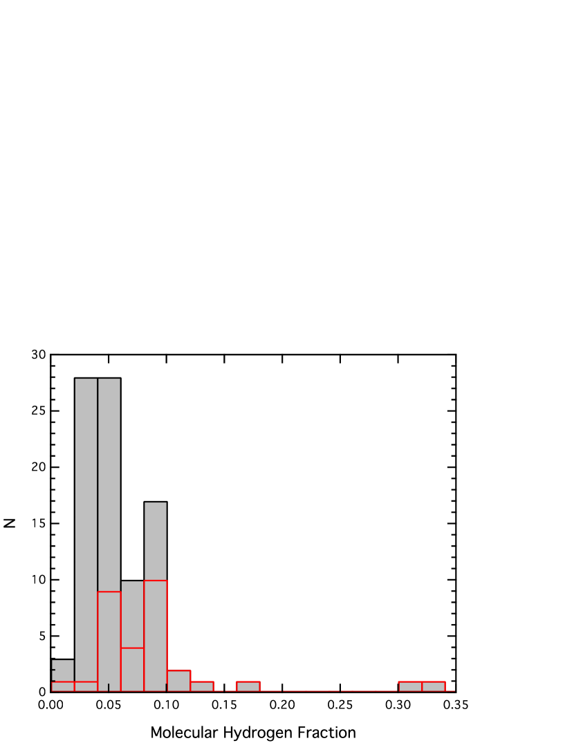
Figure 22: Distribution of $f_{\rm H_{2}}$ as determined from our analysis of OH⁺ and H₂O⁺ abundances. The filled gray bars show all velocity intervals where $f_{\rm H_{2}}$ is computed, and the red bars mark the distribution for velocity intervals within 5 km s^-1 of the systemic velocity of the background source (i.e., that may be associated with material surrounding the continuum source).

The abundance ratio $N({\rm OH}^{+})/N({\rm H_{2}O}^{+})$ is inversely related to $f_{\rm H_{2}}$, as clearly seen in equation (12). Conceptually this is easy to understand as more H₂ will drive the OH⁺ + H₂ reaction more rapidly, converting more OH⁺ into H₂O⁺. Values of $N({\rm OH}^{+})/N({\rm H_{2}O}^{+})$ and $f_{\rm H_{2}}$ are given in columns 5 and 9 of Table 5, respectively, and the distribution of $f_{\rm H_{2}}$ is presented as a histogram in Figure 22. The observed OH⁺ and H₂O⁺ abundances favor gas with low molecular hydrogen fractions, as all but three of the components in the Galactic disk have $f_{\rm H_{2}}<0.1$, and only in the Galactic center does $f_{\rm H_{2}}$ exceed 0.15. Excluding data in the Galactic center sight lines, the distribution of molecular hydrogen fractions in our sample has mean 0.053 and standard deviation 0.026.

We have also considered whether or not $f_{\rm H_{2}}$ differs in velocity intervals that are potentially associated with material surrounding our target background sources (contain absorption within 5 km s^-1 of systemic velocity). The distribution of $f_{\rm H_{2}}$ in these components is shown by the red bars in Figure 22, and it is clear that they tend to have larger molecular hydrogen fractions. If these components potentially associated with background sources are also excluded from our analysis, the mean and standard deviation of $f_{\rm H_{2}}$ in our sample change to 0.042$\pm$0.018. These results are consistent with the findings of previous studies utilizing OH⁺ and H₂O⁺ observations for the same purpose (Gerin et al., 2010b; Neufeld et al., 2010; Indriolo et al., 2012; van der Tak et al., 2013a), as well as with models of oxygen chemistry (Hollenbach et al., 2012), confirming the trend that the two species predominantly reside in mostly atomic gas.

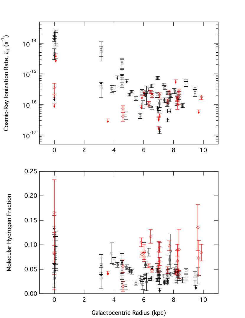
Figure 23: Top: Cosmic-ray ionization rate versus Galactocentric radius. Bottom: Molecular hydrogen fraction versus Galactocentric radius. Red diamonds denote velocity intervals within 5 km s^-1 of the systemic velocity of the background source. Black squares denote foreground clouds. Upper limits and lower limits are marked by arrows, and use the same color scheme denoting foreground versus background. Note there are 4 components, all in the Galactic center, with $f_{\rm H_{2}}>0.25$, but we have scaled the axis to more clearly show the entire data set.

A plot of the molecular hydrogen fraction versus Galactocentric radius is shown in the bottom panel of Figure 23. Red diamonds denote velocity intervals more likely associated with background sources and black squares those thought to be foreground clouds, and there is distinct separation between the bulk of the two samples as would be expected given the discussion above. There does not appear to be any relation between $f_{\rm H_{2}}$ and $R_{\rm gal}$, either for the entire sample or for the sub-samples separately. If metallicity increases toward the Galactic center though (Wolfire et al., 2003, and references therein), $x_{e}$ should as well, and larger values of $f_{\rm H_{2}}$ would be required to produce the observed $N({\rm OH}^{+})/N({\rm H_{2}O}^{+})$ ratios. Whether or not $f_{\rm H_{2}}$ changes with $R_{\rm gal}$ then hinges on the underlying assumption that $x_{e}$ is either constant or variable with Galactocentric radius.

4.5 Cosmic-ray ionization rate

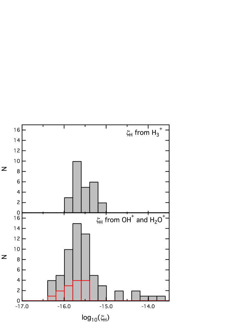
Figure 24: Histogram of $\zeta_{\rm H}$ as determined from abundances of OH⁺ and H₂O⁺ (bottom panel) and from H${}_{3}^{+}$ in diffuse clouds (top panel; Indriolo & McCall, 2012, and unpublished data). In the bottom panel filled gray bars show all velocity intervals where $\zeta_{\rm H}$ is computed, and the red bars mark the distribution for velocity intervals within 5 km s^-1 of the systemic velocity of the background source (i.e., that may be associated with material surrounding the continuum source). In the top panel, only diffuse cloud sight lines where H${}_{3}^{+}$ is detected have been used in creating the histogram of ionization rates. Over half of all sight lines observed searching for H${}_{3}^{+}$ resulted in non-detections; upper limits on the ionization rate range from a few times 10^-17 s^-1 up to 10^-15 s^-1.

The final column of Table 5 gives the cosmic-ray ionization rates inferred from our analysis, and the distribution of $\zeta_{\rm H}$ is presented in the bottom panel of Figure 24. Upper limits on $\zeta_{\rm H}$ are the result of optically thick 21 cm H i absorption that only allows us to place lower limits on $N({\rm H})$. Lower limits on $\zeta_{\rm H}$ arise when we are only able to place a lower limit on $N({\rm OH}^{+})$. A range of ionization rates is reported when H₂O⁺ is not detected, with the upper bound determined by the upper limit on $N({\rm H_{2}O^{+}})$, and the lower bound determined in the limit where $N({\rm H_{2}O^{+}})\rightarrow 0$. Uncertainties in $\zeta_{\rm H}$ only account for the uncertainties in observed column densities, and do not include the effects discussed in Section 3.6. As before, in Figure 24 the grey bars represent the total sample of velocity intervals where the ionization rate has been determined, and the red bars denote the sub-sample of clouds that may be associated with background sources. All components with $\zeta_{\rm H}>10^{-15}$ s^-1 arise in sight lines toward the Galactic center, and due to the unique nature of this region we exclude all data from the M$-$0.13$-$0.08, M$-$0.02$-$0.07, Sgr B2(M), and Sgr B2(N) sight lines during the following analysis.

The distribution of ionization rates inferred from OH⁺ and H₂O⁺ appears to be log-normal. We find the mean value of $\log(\zeta_{\rm H})$ to be -15.75 ($\zeta_{\rm H}=1.78\times 10^{-16}$ s^-1) with standard deviation 0.29. The distribution in components potentially associated with background sources does not differ appreciably, although it lacks some of the highest ionization rates seen in the foreground clouds. Shown in the top panel of Figure 24 is the distribution of ionization rates in diffuse molecular clouds found by Indriolo & McCall (2012) using observations of H${}_{3}^{+}$. Ionization rates of molecular hydrogen ($\zeta_{2}$) reported therein have been scaled by 1.5/2.3 to convert to the ionization rate of atomic hydrogen (Glassgold & Langer, 1973, 1974). This sample has a mean value of -15.55 ($\zeta_{\rm H}=2.82\times 10^{-16}$ s^-1) and standard deviation 0.24. Despite slight differences, mean ionization rates calculated using the different molecules are in agreement. To check whether or not the two distributions of ionization rates differ, we performed a two-sample K-S test, and we cannot reject the hypothesis that the two samples are drawn from the same underlying distribution. The greatest difference in the two distributions occurs for $\zeta_{\rm H}\lesssim 1.5\times 10^{-16}$ s^-1, and no ionization rates inferred from H${}_{3}^{+}$ are below $10^{-16}$ s^-1. Likely this is because H${}_{3}^{+}$ absorption lines are fairly weak (only a few percent deep at most), and at low ionization rates the molecule will not be produced in detectable abundances. This means OH⁺ and H₂O⁺ are important tracers of $\zeta_{\rm H}$ in a regime where H${}_{3}^{+}$ is unobservable.

Cosmic-ray ionization rate versus Galactocentric radius is shown in the top panel of Figure 23. Outside a radius of 5 kpc there does not seem to be any relation between $\zeta_{\rm H}$ and $R_{\rm gal}$. This appears to agree with the conclusion of a uniform cosmic-ray density drawn from gamma-ray observations tracing the flux of $E\gtrsim 300$ MeV protons (Ackermann et al., 2011). Within the Galactic center itself there is a large range of ionization rates, including six components with $\zeta_{\rm H}>10^{-14}$ s^-1. These are the highest values found in our study, and they all come from gas toward M$-$0.13$-$0.08 and M$-$0.02$-$0.07 with $-$159 km s${}^{-1}\leq v_{\rm LSR}\leq-$85 km s^-1 and toward Sgr B2(M) and Sgr B2(N) with $-$130 km s${}^{-1}\leq v_{\rm LSR}\leq-$60 km s^-1. OH⁺ shows continuous, substantial absorption over these velocities (see Figures 2–5), while H i only has minimal absorption in the same range (Figure 7 in Lang et al., 2010; Dwarakanath et al., 2004, Figure 5 position 7). As mentioned above, at such high ionization rates equation (15) is no longer a valid approximation because electrons freed during the ionization of H and H₂ make $x_{e}$ strongly dependent on $\zeta_{\rm H}$. Because our adopted value of $x_{e}$ is likely an underestimate, the high ionization rates reported in the Galactic center should still be valid lower limits. Smaller ionization rates in the Galactic center are found in the velocity intervals corresponding to all four of the background sources—regions known to be largely molecular. Indeed, the strong H₃O⁺ absorption in these components requires large H₂ abundances and denser gas. The diffuse cloud chemistry used to infer $f_{\rm H_{2}}$ and $\zeta_{\rm H}$ is almost assuredly not valid in these regions, and the higher ionization rates found in other components will be more indicative of the particle flux in the Galactic center. Previous studies of the Galactic center region also find cosmic-ray ionization rates on the order of $10^{-15}$–$10^{-13}$ s^-1. Observations of H${}_{3}^{+}$ show the molecule to be widespread in the CMZ, and inferred ionization rates are several times $10^{-15}$ s^-1 on average (Oka et al., 2005; Goto et al., 2008). Analysis of the 6.4 keV Fe K$\alpha$ line, gamma rays, and radio synchrotron emission in the Galactic center also points to a large population of energetic particles, and estimates of the resulting ionization rate range from a few times 10^-15 s^-1 up to $5\times 10^{-13}$ s^-1 depending on the location in question (Yusef-Zadeh et al., 2007, 2013).

Sight lines toward the Galactic center also show OH⁺ and H₂O⁺ absorption from the 3 kpc and 4.5 kpc spiral arms. Ionization rates in these components tend to be higher than most of those found at larger $R_{\rm gal}$, and lower than those found in the Galactic center, indicative of a gradient in $\zeta_{\rm H}$. Such a gradient was predicted by Wolfire et al. (2003), and is expected given the high concentration of energetic sources in the inner Galaxy leads to more particle acceleration than elsewhere in the disk. However, we must re-emphasize that absorption attributed to these spiral arms is very likely blended with absorption from gas within the CMZ, so it is possible that the intermediate ionization rates are simply a combination of high ionization rates in the Galactic center and average ionization rates in the spiral arms. Additional observations at $R_{\rm gal}\leq 5$ kpc are necessary to distinguish between the two interpretations.

Another relationship that has been the focus of recent studies is that between $\zeta_{\rm H}$ and $N_{\rm H}\equiv N({\rm H})+2N({\rm H}_{2})$, the total column density of a given cloud. The cross section for ionization of H and H₂ by cosmic rays increases with decreasing energy, meaning the flux of low-energy particles ($E\leq 100$ MeV) is most important in controlling $\zeta_{\rm H}$, and such particles will quickly be removed from the cosmic-ray spectrum due to these energy losses (e.g., Padovani et al., 2009). Cosmic-ray ranges (expressed as the product of density and distance, i.e., column density, through which a particle can propagate before losing all of its energy to ionization interactions) have been calculated as a function of particle energy and are available via a NIST web query. Ranges for 1 MeV, 10 MeV, and 100 MeV protons propagating through a gas of purely atomic hydrogen are $Rn({\rm H})=5.1\times 10^{20}$ cm^-2, $3.2\times 10^{22}$ cm^-2, and $2.2\times 10^{24}$ cm^-2, respectively. Given these ranges and an average diffuse cloud with $N_{\rm H}=10^{21}$ cm^-2, the higher-energy particles will pass through the entirety of the cloud, while the lower energy particles—those most important for ionization—will be stopped part of the way through the cloud. The expected result then, is that $\zeta_{\rm H}$ will decrease with increasing $N_{\rm H}$ as the particles most efficient at ionization are removed from the spectrum.

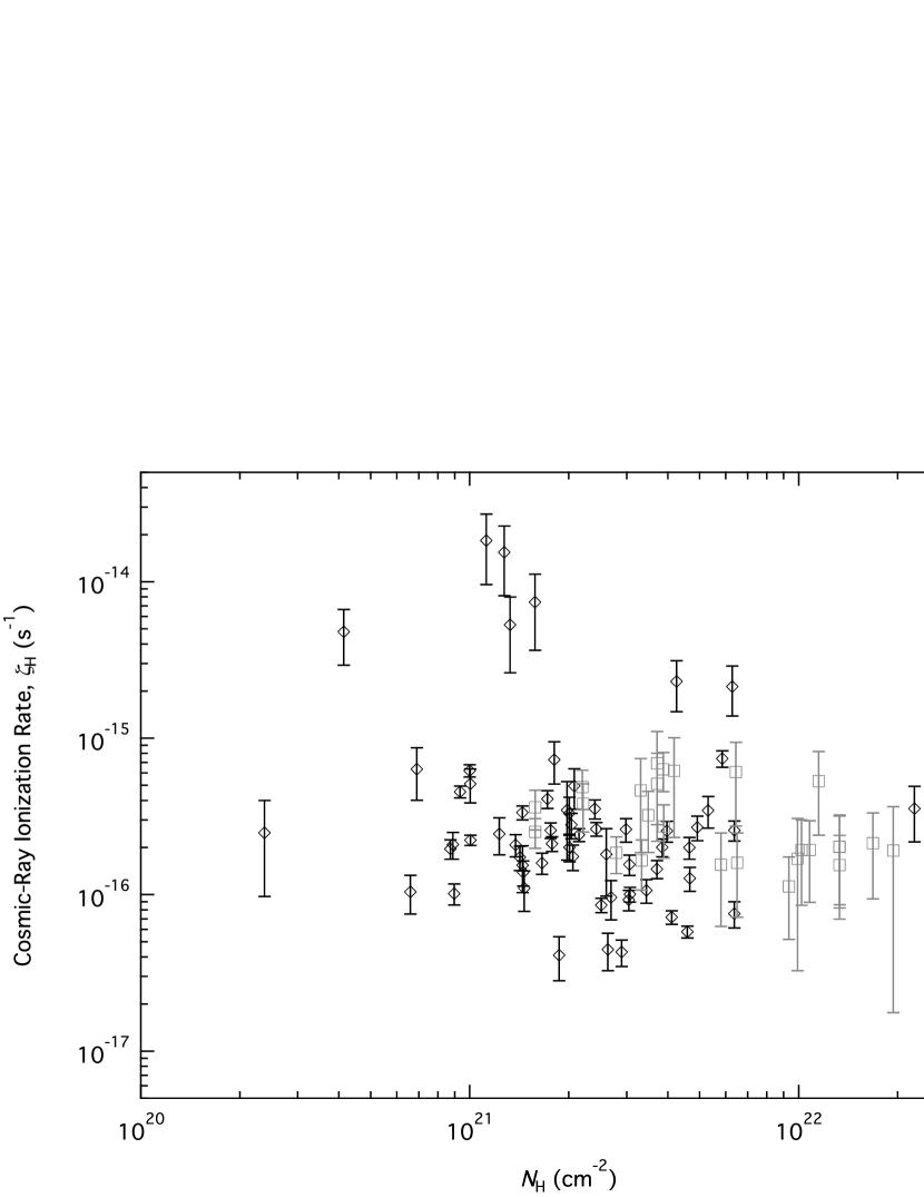
Figure 25: Cosmic-ray ionization rate versus total hydrogen column density, $N_{\rm H}$. We have estimated $N_{\rm H}$ using values of $N({\rm H})$ and $f_{\rm H_{2}}$ reported in Table 5. Black diamonds are from the present study, and grey squares from H${}_{3}^{+}$ observation of Indriolo & McCall (2012). All ionization rates above $10^{-15}$ s^-1 are from sight lines toward the Galactic center.

In Figure 25 we plot $\zeta_{\rm H}$ versus $N_{\rm H}$ for the sample studied herein, and for ionization rates determined from H${}_{3}^{+}$ observations (Indriolo & McCall, 2012). We see no change in $\zeta_{\rm H}$ over the range $N_{\rm H}=0.7$–20$\times 10^{21}$ cm^-2, consistent with our previous findings. Only for clouds with $N_{\rm H}\gtrsim 10^{23}$ cm^-2 do reported ionization rates decrease significantly (e.g., see Padovani et al., 2009, and references therein), hinting at the loss of low-energy cosmic rays. The lack of a correlation between $\zeta_{\rm H}$ and $N_{\rm H}$ in diffuse clouds may be due to multiple effects. Even if the column density along a line of sight is large enough to stop low-energy particles, it is possible that the amount of material a particle would have traverse to reach that point moving in the plane of the sky is much lower. It is also possible that what appears as a single absorption feature in velocity space is actually composed of several discrete clouds along the line of sight, each with column densities much smaller than the total. Finally, due to the small molecular hydrogen fractions we have concluded that OH⁺ and H₂O⁺ reside predominantly in the outer layers of clouds. This means that our inferred ionization rates are based on material expected to experience a mostly unattenuated flux of low-energy cosmic rays.

5 SUMMARY

We have surveyed 20 sight lines in the Galactic disk with the Herschel Space Observatory, all of which show absorption from OH⁺ and $o$-H₂O⁺. Sight lines have been sub-divided by velocity intervals into a total sample of 105 components where we determine column densities for the observed species. H₃O⁺ is detected in only 4 components outside of the Galactic center, suggesting the majority of the gas being probed is diffuse and at $A_{V}\lesssim 3$ mag. Abundances are used to infer both the molecular hydrogen fraction and cosmic-ray ionization rate in each component. The vast majority of components have $f_{\rm H_{2}}\leq 0.1$, confirming previous findings that OH⁺ and H₂O⁺ reside in primarily atomic gas, likely in the outer layers of clouds. We find a distinct difference in the distribution of $f_{\rm H_{2}}$ in foreground components versus the distribution in components potentially associated with material surrounding background sources (i.e., envelopes, outflows), with the latter showing larger molecular hydrogen fractions. The distribution of $f_{\rm H_{2}}$ in foreground components is described by a Gaussian function with mean and standard deviation $0.042\pm 0.018$. We find no correlation between molecular hydrogen fraction and Galactocentric radius, although this is dependent on the assumption of a constant $x_{e}$. If the electron fraction varies with $R_{\rm gal}$ (perhaps in unison with the known metallicity gradient), then $f_{\rm H_{2}}$ would increase toward the Galactic center.

Our study has more than doubled the sample of Galactic diffuse molecular clouds where the cosmic-ray ionization rate has been determined. Ionization rates inferred from OH⁺ and H₂O⁺ outside the Galactic center show a log-normal distribution with mean -15.75 ($\zeta_{\rm H}=1.78\times 10^{-16}$ s^-1) and standard deviation 0.29. This distribution is consistent with that found using H${}_{3}^{+}$ observations along diffuse molecular cloud sight lines, and the mean ionization rates found using the different molecular tracers agree within uncertainties. Given these results and the size of our sample, we confirm the findings that average cosmic-ray ionization rates in the Galactic disk are on the order of $10^{-16}$ s^-1.

Cosmic-ray ionization rates in the Galactic center are 1–2 orders of magnitude larger than those found in the Galactic disk, again consistent with previous findings. It is possible that there is a gradient in $\zeta_{\rm H}$, with the ionization rate decreasing from the Galactic center out to $R_{\rm gal}\approx 5$ kpc, but for $R_{\rm gal}>5$ kpc $\zeta_{\rm H}$ shows no correlation with Galactocentric radius. This is in agreement with the gamma-ray signature from $E\geq 300$ MeV protons interacting with ambient gas, and it is interesting that particles at these different energies show similar behavior despite significantly different ranges.

Support for this work was provided by NASA through an award issued by JPL/Caltech. N.I. and D.A.N. are funded by NASA Research Support Agreement No. 1393741 provided through JPL. J.R.G. thanks the Spanish MINECO for funding support under grants CSD2009-00038 and AYA2012- 32032. The authors thank Vincent Fish for providing digital copies of H i spectra from his 2003 paper, and the anonymous referee for insightful comments and suggestions. HIFI has been designed and built by a consortium of institutes and university departments from across Europe, Canada and the United States under the leadership of SRON Netherlands Institute for Space Research, Groningen, The Netherlands and with major contributions from Germany, France and the US. Consortium members are: Canada: CSA, U.Waterloo; France: CESR, LAB, LERMA, IRAM; Germany: KOSMA, MPIfR, MPS; Ireland, NUI Maynooth; Italy: ASI, IFSI-INAF, Osservatorio Astrofisico di Arcetri-INAF; Netherlands: SRON, TUD; Poland: CAMK, CBK; Spain: Observatorio Astronómico Nacional (IGN), Centro de Astrobiología (CSIC-INTA). Sweden: Chalmers University of Technology - MC2, RSS & GARD; Onsala Space Observatory; Swedish National Space Board, Stockholm University - Stockholm Observatory; Switzerland: ETH Zurich, FHNW; USA: Caltech, JPL, NHSC.

Figure 16: Same as Figure 2 but for NGC 7538 IRS 1.

Table 1: Targeted Transitions

Molecule	Transition			Rest Frequency	$E_{l}/k$	$g_{u}$	$g_{l}$	$A$
				(MHz)	(K)			(10-2 s-1)
	$N^{\prime}$–$N^{\prime\prime}$	$J^{\prime}$–$J^{\prime\prime}$	$F^{\prime}$–$F^{\prime\prime}$
OH+	1–0	0–1	1/2–1/2	1909045.2	0.0055	2	2	0.52
OH+	1–0	0–1	1/2–3/2	1909158.8	0	2	4	1.05
OH+	1–0	2–1	5/2–3/2	1971803.8	0	6	4	1.82
OH+	1–0	2–1	3/2–1/2	1971805.3	0.0055	4	2	1.52
OH+	1–0	2–1	3/2–3/2	1971919.2	0	4	4	0.30
OH+	1–0	1–1	1/2–1/2	1032997.9	0.0055	2	2	1.41
OH+	1–0	1–1	3/2–1/2	1033004.4	0.0055	4	2	0.35
OH+	1–0	1–1	1/2–3/2	1033111.8	0	2	4	0.70
OH+	1–0	1–1	3/2–3/2	1033118.6	0	4	4	1.76
	$N^{\prime}_{K^{\prime}_{a}K^{\prime}_{c}}$–$N^{\prime\prime}_{K^{\prime\prime}_{a}K^{\prime\prime}_{c}}$	$J^{\prime}$–$J^{\prime\prime}$	$F^{\prime}$–$F^{\prime\prime}$
$p$-H2O+	$1_{10}$–$1_{01}$	3/2–3/2	3/2–3/2	1607227.3	30.024	4	4	0.62
$p$-H2O+	$1_{10}$–$1_{01}$	1/2–1/2	1/2–1/2	1631724.1	30.146	2	2	0.56
$o$-H2O+	$1_{11}$–$0_{00}$	3/2–1/2	3/2–1/2	1115155.8	0.0053	4	2	1.71
$o$-H2O+	$1_{11}$–$0_{00}$	3/2–1/2	1/2–1/2	1115191.2	0.0053	2	2	2.75
$o$-H2O+	$1_{11}$–$0_{00}$	3/2–1/2	5/2–3/2	1115209.1	0	6	4	3.10
$o$-H2O+	$1_{11}$–$0_{00}$	3/2–1/2	3/2–3/2	1115267.9	0	4	4	1.39
$o$-H2O+	$1_{11}$–$0_{00}$	3/2–1/2	1/2–3/2	1115303.3	0	2	4	0.35
$o$-H2O+	$1_{11}$–$0_{00}$	1/2–1/2	1/2–1/2	1139541.5	0.0053	2	2	0.37
$o$-H2O+	$1_{11}$–$0_{00}$	1/2–1/2	3/2–1/2	1139560.6	0.0053	4	2	1.48
$o$-H2O+	$1_{11}$–$0_{00}$	1/2–1/2	1/2–3/2	1139653.7	0	2	4	2.93
$o$-H2O+	$1_{11}$–$0_{00}$	1/2–1/2	3/2–3/2	1139672.7	0	4	4	1.83
		$J_{K}^{\pm}$–$J_{K}^{\mp}$
H3O+		$1_{1}^{-}-1_{1}^{+}$		1655833.9	0	6	6	5.46
H3O+		$0_{0}^{-}-1_{0}^{+}$		1984711.9	7.3	4	12	2.30

Note. — All data were obtained from the Cologne Database for Molecular Spectroscopy (CDMS; Müller et al., 2005), although some frequencies have been updated as described below. OH⁺ data are from Bekooy et al. (1985). H₂O⁺ data are from Mürtz et al. (1998), but the frequencies for the transitions at 1115 GHz have been shifted by +5 MHz. This shift provides the best match between $o$-H₂O⁺ and OH⁺ absorption profiles in velocity space, and agrees with the findings of Neufeld et al. (2010). The H₃O⁺ transition frequencies are from Yu et al. (2009). Energy level diagrams depicting the specific states studied herein are available for OH⁺ (López-Sepulcre et al., 2013), H₂O⁺ (Schilke et al., 2010; Ossenkopf et al., 2010), and H₃O⁺ (Verhoeve et al., 1988, 1989).

Table 2: Target List

Target	Right Ascension	Declination	Gal. Long.	Gal. Lat.	Distance	Ref.
	(hh:mm:ss.s)	(dd:mm:ss.s)	(deg)	(deg)	(kpc)
M$-$0.13$-$0.08 [SgrA∗+20 km s-1 cloud]	17:45:37.4	$-$29:05:40.0	359.8653	$-$0.0831	8.34	1,2
M$-$0.02$-$0.07 [SgrA∗+50 km s-1 cloud]	17:45:50.5	$-$28:59:53.3	359.9724	$-$0.0737	8.34	1,2
Sgr B2(M)	17:47:20.6	$-$28:23:03.3	0.6681	$-$0.0364	8.34	1,3,4
Sgr B2(N)	17:47:20.1	$-$28:22:18.5	0.6778	$-$0.0284	8.34	1,3,4
W28A [G005.89$-$00.39]	18:00:30.5	$-$24:03:59.9	5.8857	$-$0.3924	1.28	5
W31C [G010.62$-$00.38]	18:10:28.7	$-$19:55:50.0	10.6234	$-$0.3838	4.95	6
W33A [G012.91$-$00.26]	18:14:39.2	$-$17:52:00.5	12.9078	$-$0.2592	2.4	7
G029.96$-$00.02	18:46:03.8	$-$02:39:22.0	29.9556	$-$0.0163	5.26	8
G034.3+00.15	18:53:18.6	$+$01:14:58.0	34.2577	0.1521	3.8	9
W49N	19:10:13.1	$+$09:06:12.5	43.1657	0.0123	11.11	10
W51e	19:23:43.6	$+$14:30:29.2	49.4879	$-$0.3871	5.41	11
AFGL 2591	20:29:24.7	$+$40:11:18.7	78.8862	0.7091	3.33	12
DR21C	20:39:01.1	$+$42:19:43.0	81.6810	0.5394	1.5	12
DR21(OH)	20:39:00.9	$+$42:22:48.6	81.7214	0.5713	1.5	12
NGC 7538 IRS1 [G111.54$+$00.78]	23:13:45.7	$+$61:28:21.0	111.5438	0.7794	2.65	13
W3 IRS5	02:25:40.6	$+$62:05:51.0	133.7168	1.2156	1.83	14
W3(OH)	02:27:03.8	$+$61:52:24.6	133.9473	1.0642	2.04	15
G327.30$-$00.60	15:53:08.7	$-$54:36:58.6	327.3042	-0.5515	3.3	16
NGC 6334 I	17:20:53.5	$-$35:47:01.0	351.4172	0.6448	1.35	17
NGC 6334 I(N)	17:20:54.8	$-$35:45:09.6	351.4452	0.6589	1.35	17

Note. — Names in brackets are alternate identifiers for the targets. All coordinates are in the J2000.0 system and indicate where the telescope was pointed. They may not exactly match published coordinates for the background sources, but in all cases pointings are close enough that the sources are well within the telescope beam (about 19″, 22″, and 34″ FWHM at 1100 GHz, 950 GHz, and 600 GHz, respectively). Distance references are given below; unless otherwise noted, distance determinations are from trigonometric parallax.
References: 1-Reid et al. (2014); 2-Ferrière (2012); 3-Reid et al. (2009); 4-Molinari et al. (2011); 5-Motogi et al. (2011); 6-Sanna et al. (2014); 7-Immer et al. (2013); 8-Zhang et al. (2014); 9-Fish et al. (2003, kinematic analysis); 10-Zhang et al. (2013); 11-Sato et al. (2010); 12-Rygl et al. (2012); 13-Moscadelli et al. (2009); 14-Imai et al. (2000); 15-Hachisuka et al. (2006); 16-Urquhart et al. (2012, kinematic analysis); 17-Wu et al. (2014)

Table 3: Double Side Band Continuum Level Antenna Temperature and RMS Noise

Source	909 GHz	971 GHz	1033 GHz	1115 GHz	607 GHz	631 GHz	984 GHz
	$T_{A}({\rm DSB})$	$T_{A}({\rm DSB})$	$T_{A}({\rm DSB})$	$T_{A}({\rm DSB})$	$T_{A}({\rm DSB})$	$T_{A}({\rm DSB})$	$T_{A}({\rm DSB})$
	(K)	(K)	(K)	(K)	(K)	(K)	(K)
M$-$0.13$-$0.08	…	1.45$\pm$0.07	…	1.40$\pm$0.07	…	…	1.45$\pm$0.05
M$-$0.02$-$0.07	…	0.85$\pm$0.02	…	0.90$\pm$0.03	0.44$\pm$0.02	0.51$\pm$0.02	0.90$\pm$0.02
Sgr B2(M)	17.53$\pm$0.11	19.34$\pm$0.31	20.63$\pm$0.21	22.86$\pm$0.21	…	…	19.63$\pm$0.22
Sgr B2(N)	16.60$\pm$0.12	17.86$\pm$0.20	17.99$\pm$0.19	19.07$\pm$0.38	…	…	17.86$\pm$0.20
W28A	…	3.78$\pm$0.03	…	5.47$\pm$0.04	1.01$\pm$0.02	…	3.76$\pm$0.03
W31C	4.87$\pm$0.04	5.46$\pm$0.04	…	6.45$\pm$0.08	1.55$\pm$0.01	1.75$\pm$0.01	5.44$\pm$0.04
W33A	…	1.73$\pm$0.02	…	2.18$\pm$0.01	0.54$\pm$0.01	0.61$\pm$0.01	1.72$\pm$0.01
G029.96$-$00.02	1.74$\pm$0.01	2.08$\pm$0.02	…	2.80$\pm$0.03	0.51$\pm$0.01	…	2.11$\pm$0.03
G034.3+00.15	5.83$\pm$0.04	6.25$\pm$0.05	…	8.94$\pm$0.02	2.26$\pm$0.02	2.27$\pm$0.03	6.32$\pm$0.06
W49N	6.36$\pm$0.03	8.08$\pm$0.05	…	9.55$\pm$0.12	2.34$\pm$0.01	2.60$\pm$0.03	8.10$\pm$0.07
W51e	7.43$\pm$0.05	8.20$\pm$0.03	…	10.10$\pm$0.05	2.62$\pm$0.01	2.91$\pm$0.03	8.13$\pm$0.03
AFGL 2591	…	…	1.38$\pm$0.02	1.71$\pm$0.02	…	…	1.18$\pm$0.03
DR21C	2.01$\pm$0.03	2.50$\pm$0.04	…	2.91$\pm$0.03	0.90$\pm$0.01	…	2.52$\pm$0.04
DR21(OH)	…	3.83$\pm$0.02	…	5.08$\pm$0.03	1.20$\pm$0.02	1.32$\pm$0.02	3.80$\pm$0.03
NGC 7538 IRS1	…	1.96$\pm$0.05	2.41$\pm$0.02	2.74$\pm$0.02	…	…	…
W3 IRS5	…	2.19$\pm$0.04	2.61$\pm$0.02	3.09$\pm$0.02	0.61$\pm$0.01	…	…
W3(OH)	2.64$\pm$0.02	3.09$\pm$0.02	…	4.14$\pm$0.02	0.89$\pm$0.01	…	3.11$\pm$0.03
G327.30$-$00.60	…	4.71$\pm$0.03	…	5.26$\pm$0.02	…	…	…
NGC 6334 I	…	…	9.17$\pm$0.04	10.81$\pm$0.05	…	…	…
NGC 6334 I(N)	…	…	4.58$\pm$0.02	4.53$\pm$0.02	…	…	…

Note. — Shown here is the continuum level double sideband antenna temperature and root mean square (RMS) noise resulting from the combination of all observations of each transition. The full list of ObsIDs used to generate the final spectrum for each transition is given in Table A1.

Table 4: Derived column densities

Source	$v_{\rm LSR}$ range	$N({\rm OH}^{+})$	$N({\rm OH}^{+})$	$N({\rm OH}^{+})$	$N(o$-${\rm H_{2}O^{+}})$	$N(p$-${\rm H_{2}O^{+}})$	$N(p$-${\rm H_{2}O^{+}})$	H2O+ OPR	H3O+ $N(1_{0}^{+})$
		909 GHz	971 GHz	1033 GHz	1115 GHz	607 GHz	631 GHz		984 GHz
	(km s-1)	($10^{13}$ cm-2)	($10^{13}$ cm-2)	($10^{13}$ cm-2)	($10^{13}$ cm-2)	($10^{13}$ cm-2)	($10^{13}$ cm-2)		($10^{13}$ cm-2)
M$-$0.13$-$0.08	[-210, -159]	…	$>$7.88	…	2.40$\pm$1.38	…	…	…	…
M$-$0.13$-$0.08	[-159, -133]	…	$>$16.88	…	12.59$\pm$4.94	…	…	…	…
M$-$0.13$-$0.08	[-133, -92]	…	$>$23.95	…	12.29$\pm$3.52	…	…	…	…
M$-$0.13$-$0.08	[-92, -50]	…	$>$22.49	…	4.16$\pm$1.40	…	…	…	$<$2.98
M$-$0.13$-$0.08	[-50, -39]	…	5.11$\pm$1.42	…	0.51$\pm$0.29	…	…	…	$<$0.78
M$-$0.13$-$0.08	[-39, -14]	…	$>$10.79	…	2.12$\pm$0.80	…	…	…	$<$1.77
M$-$0.13$-$0.08	[-14, 21]	…	20.77$\pm$6.20	…	4.67$\pm$1.39	…	…	…	2.40$\pm$2.92
M$-$0.13$-$0.08	[21, 33]	…	1.96$\pm$0.55	…	0.45$\pm$0.30	…	…	…	$<$0.85
M$-$0.02$-$0.07	[-215, -151]	…	19.84$\pm$3.85	…	1.97$\pm$1.07	$<$1.24	$<$5.74	…	…
M$-$0.02$-$0.07	[-151, -121]	…	$>$24.32	…	8.16$\pm$1.69	2.77$\pm$1.57	2.38$\pm$3.00	3.04$\pm$1.69	…
M$-$0.02$-$0.07	[-121, -85]	…	$>$25.00	…	4.79$\pm$0.98	$<$1.80	$<$3.54	…	…
M$-$0.02$-$0.07	[-85, -61]	…	14.79$\pm$2.45	…	1.47$\pm$0.46	$<$1.18	$<$2.36	…	$<$0.48
M$-$0.02$-$0.07	[-61, -47]	…	$>$8.14	…	1.07$\pm$0.29	$<$0.72	$<$1.37	…	$<$0.28
M$-$0.02$-$0.07	[-47, -37]	…	3.96$\pm$0.50	…	0.30$\pm$0.17	$<$0.50	$<$0.95	…	$<$0.20
M$-$0.02$-$0.07	[-37, -23]	…	7.18$\pm$1.10	…	1.06$\pm$0.29	$<$0.71	$<$1.33	…	$<$0.28
M$-$0.02$-$0.07	[-23, -13]	…	6.16$\pm$0.98	…	0.81$\pm$0.21	$<$0.48	$<$1.01	…	$<$0.20
M$-$0.02$-$0.07	[-13, 20]	…	19.08$\pm$3.13	…	2.63$\pm$0.70	$<$1.72	$<$3.20	…	$<$0.66
M$-$0.02$-$0.07	[20, 75]	…	14.21$\pm$1.92	…	5.42$\pm$1.30	$<$1.95	$<$5.12	…	4.18$\pm$1.57
Sgr B2(M)	[-130, -57]	…	…	…	…	…	…	…	1.67$\pm$0.33
Sgr B2(M)	[-57, -33]	…	…	…	…	…	…	2.68$\pm$0.76	0.31$\pm$0.06
Sgr B2(M)	[-33, -2]	…	…	…	…	…	…	2.83$\pm$0.80	0.76$\pm$0.15
Sgr B2(M)	[-2, 40]	…	…	…	…	…	…	2.83$\pm$0.80	1.47$\pm$0.29
Sgr B2(M)	[40, 100]	…	…	…	…	…	…	…	7.02$\pm$1.40
Sgr B2(N)	[-130, -60]	…	…	…	…	…	…	…	3.99$\pm$0.80
Sgr B2(N)	[-60, -31]	…	…	…	…	…	…	…	1.47$\pm$0.29
Sgr B2(N)	[-31, -7]	…	…	…	…	…	…	…	0.27$\pm$0.05
Sgr B2(N)	[-7, 36]	…	…	…	…	…	…	…	1.50$\pm$0.30
Sgr B2(N)	[36, 100]	…	…	…	…	…	…	…	12.57$\pm$2.51
W28A	[-3, 11]	…	2.19$\pm$0.10	…	0.41$\pm$0.04	$<$0.24	…	…	$<$0.19
W28A	[11, 18]	…	1.27$\pm$0.06	…	0.32$\pm$0.02	…	…	…	$<$0.11
W28A	[18, 28]	…	0.73$\pm$0.05	…	$<$0.03	…	…	…	$<$0.15
W31C	[-20, -1]	$<$0.39	0.72$\pm$0.09	…	$<$0.10	…	…	…	$<$0.14
W31C	[-1, 12]	8.42$\pm$0.44	8.92$\pm$0.80	…	1.14$\pm$0.10	…	…	…	$<$0.11
W31C	[12, 24]	7.91$\pm$0.40	7.65$\pm$0.50	…	1.49$\pm$0.11	…	…	…	0.58$\pm$0.19
W31C	[24, 36]	9.97$\pm$0.46	$>$10.50	…	1.58$\pm$0.12	…	$<$0.20	…	$<$0.19
W31C	[36, 43]	8.37$\pm$0.36	$>$7.11	…	1.45$\pm$0.10	0.49$\pm$0.04	0.26$\pm$0.11	2.98$\pm$0.34	0.48$\pm$0.12
W31C	[43, 60]	2.35$\pm$0.39	2.37$\pm$0.15	…	0.50$\pm$0.10	0.22$\pm$0.10	$<$0.25	2.26$\pm$1.09	$<$0.18
W33A	[-4, 18]	…	0.85$\pm$0.14	…	0.20$\pm$0.06	$<$0.14	$<$0.91	…	$<$0.38
W33A	[18, 25]	…	0.60$\pm$0.06	…	0.14$\pm$0.02	$<$0.09	$<$0.30	…	$<$0.12
W33A	[25, 36]	…	1.99$\pm$0.12	…	0.42$\pm$0.03	$<$0.11	…	…	$<$0.19
W33A	[36, 50]	…	1.44$\pm$0.12	…	0.33$\pm$0.04	…	…	…	$<$0.24
G029.96$-$00.02	[-10, 6]	1.71$\pm$0.34	1.56$\pm$0.11	…	0.17$\pm$0.07	$<$0.18	…	…	$<$0.53
G029.96$-$00.02	[6, 17]	2.41$\pm$0.25	2.22$\pm$0.11	…	0.44$\pm$0.05	$<$0.12	…	…	$<$0.36
G029.96$-$00.02	[17, 28]	0.84$\pm$0.23	1.25$\pm$0.08	…	0.12$\pm$0.05	$<$0.12	…	…	$<$0.36
G029.96$-$00.02	[28, 38]	0.35$\pm$0.20	0.24$\pm$0.05	…	$<$0.04	$<$0.11	…	…	$<$0.33
G029.96$-$00.02	[38, 45]	0.58$\pm$0.14	0.52$\pm$0.04	…	0.04$\pm$0.03	$<$0.08	…	…	$<$0.23
G029.96$-$00.02	[45, 50]	0.81$\pm$0.11	0.68$\pm$0.04	…	0.04$\pm$0.02	$<$0.06	…	…	$<$0.17
G029.96$-$00.02	[50, 56]	1.17$\pm$0.13	0.97$\pm$0.05	…	0.09$\pm$0.03	$<$0.07	…	…	$<$0.20
G029.96$-$00.02	[56, 65]	2.85$\pm$0.22	2.49$\pm$0.11	…	0.17$\pm$0.04	$<$0.10	…	…	$<$0.30
G029.96$-$00.02	[65, 73]	3.60$\pm$0.22	3.92$\pm$0.25	…	0.51$\pm$0.04	$<$0.18	…	…	$<$0.27
G029.96$-$00.02	[73, 79]	2.04$\pm$0.15	2.14$\pm$0.10	…	0.30$\pm$0.03	$<$0.15	…	…	$<$0.20
G029.96$-$00.02	[79, 88]	1.06$\pm$0.19	1.29$\pm$0.07	…	0.07$\pm$0.04	$<$0.10	…	…	$<$0.30
G029.96$-$00.02	[88, 95]	0.54$\pm$0.14	0.90$\pm$0.05	…	0.04$\pm$0.03	$<$0.08	…	…	$<$0.24
G029.96$-$00.02	[95, 113]	2.16$\pm$0.38	2.43$\pm$0.14	…	0.39$\pm$0.08	…	…	…	$<$0.62
G034.3+00.15	[-12, 7]	3.18$\pm$0.38	2.42$\pm$0.14	…	0.20$\pm$0.02	$<$0.15	$<$0.55	…	$<$0.40
G034.3+00.15	[7, 18]	2.62$\pm$0.23	3.06$\pm$0.13	…	0.41$\pm$0.01	$<$0.16	$<$0.33	…	$<$0.23
G034.3+00.15	[18, 36]	2.90$\pm$0.36	2.67$\pm$0.13	…	0.23$\pm$0.02	$<$0.15	$<$0.55	…	$<$0.37
G034.3+00.15	[36, 44]	1.83$\pm$0.17	1.68$\pm$0.07	…	0.16$\pm$0.01	$<$0.06	$<$0.25	…	$<$0.16
G034.3+00.15	[44, 52]	3.71$\pm$0.20	3.63$\pm$0.18	…	0.65$\pm$0.01	0.19$\pm$0.07	…	3.36$\pm$1.16	$<$0.17
G034.3+00.15	[52, 70]	5.26$\pm$0.40	3.91$\pm$0.20	…	0.92$\pm$0.03	…	…	…	$<$0.38
W49N	[-10, 1]	0.39$\pm$0.14	0.62$\pm$0.05	…	$<$0.06	$<$0.07	…	…	$<$0.19
W49N	[1, 10]	3.37$\pm$0.15	3.27$\pm$0.13	…	0.48$\pm$0.06	$<$0.05	…	…	$<$0.16
W49N	[10, 17]	3.16$\pm$0.12	3.00$\pm$0.11	…	0.80$\pm$0.06	…	…	…	$<$0.14
W49N	[17, 25]	7.45$\pm$0.20	$>$6.47	…	0.58$\pm$0.06	…	…	…	$<$0.15
W49N	[25, 43]	24.40$\pm$0.65	$>$16.77	…	3.48$\pm$0.26	…	…	…	$<$0.35
W49N	[43, 51]	5.18$\pm$0.16	5.66$\pm$0.46	…	0.53$\pm$0.06	0.17$\pm$0.05	$<$0.21	3.18$\pm$1.01	$<$0.15
W49N	[51, 66]	11.59$\pm$0.33	$>$13.06	…	1.34$\pm$0.12	0.32$\pm$0.10	$<$0.39	4.21$\pm$1.31	$<$0.29
W49N	[66, 80]	6.01$\pm$0.25	$>$6.75	…	0.57$\pm$0.09	$<$0.09	…	…	$<$0.26
W51e	[-4, 11]	3.87$\pm$0.31	3.25$\pm$0.08	…	0.45$\pm$0.04	0.15$\pm$0.06	$<$0.44	2.95$\pm$1.15	$<$0.11
W51e	[11, 16]	1.36$\pm$0.10	1.10$\pm$0.02	…	0.13$\pm$0.01	$<$0.02	$<$0.14	…	$<$0.03
W51e	[16, 21]	0.99$\pm$0.10	0.84$\pm$0.02	…	0.06$\pm$0.01	$<$0.02	$<$0.14	…	$<$0.04
W51e	[21, 33]	2.00$\pm$0.23	1.84$\pm$0.05	…	0.13$\pm$0.03	$<$0.04	$<$0.35	…	$<$0.09
W51e	[33, 42]	0.99$\pm$0.17	0.96$\pm$0.03	…	0.15$\pm$0.02	$<$0.03	$<$0.26	…	$<$0.06
W51e	[42, 55]	4.91$\pm$0.30	5.28$\pm$0.14	…	0.74$\pm$0.04	…	…	…	$<$0.09
W51e	[55, 62]	1.79$\pm$0.14	1.78$\pm$0.04	…	0.30$\pm$0.02	…	…	…	0.17$\pm$0.05
W51e	[62, 75]	2.54$\pm$0.26	2.02$\pm$0.06	…	0.47$\pm$0.03	…	…	…	0.22$\pm$0.10
AFGL 2591	[-30, -7]	…	…	1.55$\pm$0.38	0.38$\pm$0.11	…	…	…	$<$1.02
AFGL 2591	[-7, 23]	…	…	8.65$\pm$0.96	1.03$\pm$0.16	…	…	…	$<$1.66
DR21C	[-16, -5]	1.23$\pm$0.45	1.10$\pm$0.15	…	0.21$\pm$0.05	$<$0.14	…	…	$<$0.38
DR21C	[-5, 3]	3.57$\pm$0.43	3.53$\pm$0.40	…	0.47$\pm$0.04	$<$0.11	…	…	$<$0.28
DR21C	[3, 21]	9.98$\pm$1.06	8.81$\pm$1.35	…	1.21$\pm$0.10	0.26$\pm$0.14	…	4.58$\pm$2.40	$<$0.64
DR21(OH)	[-20, -5]	…	1.58$\pm$0.06	…	0.38$\pm$0.04	$<$0.24	$<$0.00	…	$<$0.23
DR21(OH)	[-5, 3]	…	4.50$\pm$0.18	…	0.63$\pm$0.03	…	…	…	$<$0.12
DR21(OH)	[3, 25]	…	9.36$\pm$0.60	…	1.31$\pm$0.07	…	…	…	$<$0.34
NGC 7538 IRS1	[-65, -39]	…	0.94$\pm$0.40	1.39$\pm$0.28	0.41$\pm$0.07	…	…	…	…
NGC 7538 IRS1	[-39, -31]	…	0.42$\pm$0.13	0.49$\pm$0.09	0.05$\pm$0.02	…	…	…	…
NGC 7538 IRS1	[-31, -20]	…	0.52$\pm$0.17	0.47$\pm$0.12	$<$0.03	…	…	…	…
NGC 7538 IRS1	[-17, -3]	…	2.61$\pm$0.40	2.20$\pm$0.19	0.20$\pm$0.04	…	…	…	…
NGC 7538 IRS1	[-3, 18]	…	2.88$\pm$0.49	2.38$\pm$0.26	0.27$\pm$0.06	…	…	…	…
W3 IRS5	[-55, -35]	…	0.63$\pm$0.21	0.79$\pm$0.13	0.15$\pm$0.06	…	…	…	…
W3 IRS5	[-28, -8]	…	2.99$\pm$0.30	2.79$\pm$0.14	0.20$\pm$0.05	…	…	…	…
W3 IRS5	[-8, 10]	…	4.30$\pm$0.45	3.63$\pm$0.16	0.39$\pm$0.06	$<$0.11	…	…	…
W3(OH)	[-51, -39]	0.82$\pm$0.19	0.87$\pm$0.05	…	0.20$\pm$0.03	…	…	…	$<$0.23
W3(OH)	[-25, -8]	2.30$\pm$0.28	3.09$\pm$0.10	…	0.38$\pm$0.05	…	…	…	$<$0.34
W3(OH)	[-8, 9]	3.72$\pm$0.30	3.53$\pm$0.12	…	0.50$\pm$0.05	$<$0.17	…	…	$<$0.34
G327.3$-$0.6	[-57, -40]	…	2.71$\pm$0.10	…	0.74$\pm$0.04	…	…	…	…
G327.3$-$0.6	[-40, -28]	…	1.16$\pm$0.06	…	0.35$\pm$0.02	…	…	…	…
G327.3$-$0.6	[-28, -15]	…	2.92$\pm$0.12	…	0.32$\pm$0.03	…	…	…	…
G327.3$-$0.6	[-15, -8]	…	1.48$\pm$0.05	…	0.17$\pm$0.01	…	…	…	…
G327.3$-$0.6	[-8, 6]	…	1.59$\pm$0.07	…	0.25$\pm$0.03	…	…	…	…
NGC 6334 I	[-17, -7]	…	…	0.47$\pm$0.04	0.11$\pm$0.02	…	…	…	…
NGC 6334 I	[-7, 1]	…	…	1.83$\pm$0.05	0.26$\pm$0.02	…	…	…	…
NGC 6334 I	[1, 14]	…	…	1.84$\pm$0.07	0.23$\pm$0.03	…	…	…	…
NGC 6334 I(N)	[-9, 1]	…	…	1.68$\pm$0.05	0.28$\pm$0.02	…	…	…	…
NGC 6334 I(N)	[1, 12]	…	…	1.88$\pm$0.06	0.20$\pm$0.02	…	…	…	…

Note. — Column densities in the indicated velocity intervals determined from individual transitions of OH⁺, H₂O⁺, and H₃O⁺ are presented here. Because the total OH⁺ and H₂O⁺ column densities for Sgr B2(M) and Sgr B2(N) are determined by simultaneously fitting all available transitions, we do not report individual column densities in those sight lines. Also shown are ortho-to-para ratios for H₂O⁺ in cases where $p$-H₂O⁺ is detected. For Sgr B2(M) ortho-to-para ratios are determined using the data from Schilke et al. (2013). Upper limits are given when absorption lines are not detected, and lower limits are given when the absorption features are saturated; both are reported at the $1\sigma$ level.

Table 5: Total column densities and inferred results

Source	$v_{\rm LSR}$ range	$N({\rm OH}^{+})$	$N({\rm H_{2}O^{+}})$	$N({\rm OH}^{+})/N({\rm H_{2}O^{+}})$	$N({\rm H})$	$R_{gal}$	$d$	$f_{\rm H_{2}}$	$\zeta_{\rm H}$
	(km s-1)	($10^{13}$ cm-2)	($10^{13}$ cm-2)		($10^{21}$ cm-2)	(kpc)	(kpc)		($10^{-16}$ s-1)
M$-$0.13$-$0.08	[-210, -159]	$>$7.88	3.20$\pm$1.83	$\geq$2.46	$<$0.84	0.0	8.3	$<$0.121	$>$33.13
M$-$0.13$-$0.08	[-159, -133]	$>$16.88	16.78$\pm$6.59	$\geq$1.01	2.29$\pm$0.43	0.0	8.3	$<$0.595	$>$114.09
M$-$0.13$-$0.08	[-133, -92]	$>$23.95	16.38$\pm$4.70	$\geq$1.46	1.18$\pm$0.68	0.0	8.3	$<$0.267	$>$147.29
M$-$0.13$-$0.08	[-92, -50]	$>$22.49	5.55$\pm$1.86	$\geq$4.05	$>$5.66	0.0	8.3	$<$0.065	…
M$-$0.13$-$0.08	[-50, -39]	5.11$\pm$1.42	0.68$\pm$0.38	7.51$\pm$4.73	1.91$\pm$0.18	3.1	5.2	0.032$\pm$0.022	3.47$\pm$1.81
M$-$0.13$-$0.08	[-39, -14]	$>$10.79	2.82$\pm$1.06	$\geq$3.83	3.24$\pm$0.41	4.5	3.8	$<$0.069	$>$7.46
M$-$0.13$-$0.08	[-14, 21]	20.77$\pm$6.20	6.23$\pm$1.85	3.33$\pm$1.40	$>$25.76	0.0	8.3	0.082$\pm$0.043	$<$2.06
M$-$0.13$-$0.08	[21, 33]	1.96$\pm$0.55	0.60$\pm$0.40	3.26$\pm$2.37	$>$4.87	0.0	8.3	0.084$\pm$0.076	$<$1.05
M$-$0.02$-$0.07	[-215, -151]	19.84$\pm$3.85	2.63$\pm$1.43	7.54$\pm$4.35	…	0.0	8.3	0.032$\pm$0.020	…
M$-$0.02$-$0.07	[-151, -121]	$>$24.32	10.85$\pm$2.19	$\geq$2.24	0.68$\pm$0.13	0.0	8.3	$<$0.138	$>$142.40
M$-$0.02$-$0.07	[-121, -85]	$>$25.00	6.38$\pm$1.31	$\geq$3.92	0.30$\pm$0.15	0.0	8.3	$<$0.067	$>$182.82
M$-$0.02$-$0.07	[-85, -61]	14.79$\pm$2.45	1.96$\pm$0.61	7.54$\pm$2.66	0.40$\pm$0.10	0.0	8.3	0.032$\pm$0.012	47.80$\pm$18.60
M$-$0.02$-$0.07	[-61, -47]	$>$8.14	1.43$\pm$0.39	$\geq$5.69	3.19$\pm$0.06	3.1	5.2	$<$0.044	$>$4.06
M$-$0.02$-$0.07	[-47, -37]	3.96$\pm$0.50	0.39$\pm$0.22	10.07$\pm$5.83	0.67$\pm$0.04	4.5	3.8	0.023$\pm$0.015	6.35$\pm$2.33
M$-$0.02$-$0.07	[-37, -23]	7.18$\pm$1.10	1.41$\pm$0.38	5.09$\pm$1.59	1.72$\pm$0.06	4.5	3.8	0.050$\pm$0.018	7.28$\pm$2.19
M$-$0.02$-$0.07	[-23, -13]	6.16$\pm$0.98	1.09$\pm$0.29	5.67$\pm$1.74	1.99$\pm$0.04	4.5	3.8	0.044$\pm$0.015	4.95$\pm$1.43
M$-$0.02$-$0.07	[-13, 20]	19.08$\pm$3.13	3.51$\pm$0.93	5.43$\pm$1.69	$>$18.23	0.0	8.3	0.046$\pm$0.016	$<$1.73
M$-$0.02$-$0.07	[20, 75]	14.21$\pm$1.92	7.22$\pm$1.73	1.97$\pm$0.54	18.75$\pm$0.24	0.0	8.3	0.166$\pm$0.067	3.54$\pm$1.37
Sgr B2(M)	[-130, -57]	78.74$\pm$15.75	21.33$\pm$4.27	3.69$\pm$1.04	1.18$\pm$0.39	0.1	8.3	0.072$\pm$0.025	154.25$\pm$72.89
Sgr B2(M)	[-57, -33]	34.83$\pm$6.97	7.63$\pm$1.19	4.57$\pm$1.16	1.25$\pm$0.51	3.1	5.2	0.056$\pm$0.017	53.10$\pm$26.87
Sgr B2(M)	[-33, -2]	60.33$\pm$12.07	14.59$\pm$2.29	4.13$\pm$1.05	5.89$\pm$1.04	4.5	3.8	0.063$\pm$0.019	21.35$\pm$7.52
Sgr B2(M)	[-2, 40]	34.99$\pm$7.00	11.22$\pm$1.76	3.12$\pm$0.79	…	0.1	8.3	0.089$\pm$0.028	…
Sgr B2(M)	[40, 100]	17.60$\pm$3.52	13.01$\pm$2.60	1.35$\pm$0.38	$>$4.56	0.1	8.3	0.307$\pm$0.164	$<$31.88
Sgr B2(N)	[-130, -60]	75.34$\pm$15.07	22.19$\pm$4.44	3.39$\pm$0.96	1.03$\pm$0.34	0.1	8.3	0.080$\pm$0.028	183.18$\pm$87.45
Sgr B2(N)	[-60, -31]	54.59$\pm$10.92	12.71$\pm$2.54	4.29$\pm$1.21	1.48$\pm$0.58	3.1	5.2	0.060$\pm$0.020	74.09$\pm$37.62
Sgr B2(N)	[-31, -7]	44.94$\pm$8.99	10.64$\pm$2.13	4.22$\pm$1.19	3.99$\pm$0.62	4.5	3.8	0.062$\pm$0.021	23.01$\pm$8.25
Sgr B2(N)	[-7, 36]	37.59$\pm$7.52	12.56$\pm$2.51	2.99$\pm$0.85	…	0.1	8.3	0.094$\pm$0.034	…
Sgr B2(N)	[36, 100]	22.83$\pm$4.57	17.41$\pm$3.48	1.31$\pm$0.37	$>$4.36	0.1	8.3	0.326$\pm$0.179	$<$45.71
W28A	[-3, 11]	2.19$\pm$0.10	0.55$\pm$0.05	3.96$\pm$0.39	$>$9.49	7.1	1.3	0.066$\pm$0.008	$<$0.50
W28A	[11, 18]	1.27$\pm$0.06	0.43$\pm$0.03	2.97$\pm$0.25	1.82$\pm$0.30	7.1	1.3	0.095$\pm$0.010	2.01$\pm$0.39
W28A	[18, 28]	0.73$\pm$0.05	$<$0.03	$\geq$20.94	3.17$\pm$0.43	7.1	1.3	$<$0.011	$0.11\leq\zeta_{\rm H}\leq 0.18$
W31C	[-20, -1]	0.72$\pm$0.09	$<$0.13	$\geq$5.45	$>$3.53	3.6	5.0	$<$0.046	$<$0.34
W31C	[-1, 12]	8.53$\pm$0.38	1.52$\pm$0.14	5.63$\pm$0.57	$>$2.12	8.1	0.2	0.044$\pm$0.005	$<$6.46
W31C	[12, 24]	7.81$\pm$0.31	1.99$\pm$0.15	3.93$\pm$0.34	4.95$\pm$1.04	4.0	4.5	0.067$\pm$0.007	3.44$\pm$0.79
W31C	[24, 36]	9.97$\pm$0.46	2.11$\pm$0.15	4.73$\pm$0.41	$>$2.81	4.9	3.6	0.054$\pm$0.005	$<$6.57
W31C	[36, 43]	8.37$\pm$0.36	1.91$\pm$0.11	4.39$\pm$0.31	$>$1.91	4.2	4.3	0.059$\pm$0.005	$<$8.65
W31C	[43, 60]	2.37$\pm$0.14	0.71$\pm$0.14	3.31$\pm$0.68	1.84$\pm$0.29	3.9	4.7	0.083$\pm$0.021	3.31$\pm$0.88
W33A	[-4, 18]	0.85$\pm$0.14	0.27$\pm$0.07	3.18$\pm$1.03	$>$3.19	7.8	0.6	0.087$\pm$0.035	$<$0.72
W33A	[18, 25]	0.60$\pm$0.06	0.19$\pm$0.02	3.16$\pm$0.51	$>$0.60	6.0	2.4	0.087$\pm$0.018	$<$2.71
W33A	[25, 36]	1.99$\pm$0.12	0.56$\pm$0.04	3.59$\pm$0.35	$>$1.61	6.0	2.4	0.075$\pm$0.009	$<$2.94
W33A	[36, 50]	1.44$\pm$0.12	0.44$\pm$0.05	3.25$\pm$0.46	$>$1.56	6.0	2.4	0.085$\pm$0.015	$<$2.42
G029.96$-$00.02	[-10, 6]	1.57$\pm$0.10	0.23$\pm$0.09	6.97$\pm$2.74	1.40$\pm$0.23	8.3	0.1	0.035$\pm$0.015	1.54$\pm$0.51
G029.96$-$00.02	[6, 17]	2.25$\pm$0.10	0.59$\pm$0.07	3.83$\pm$0.48	3.45$\pm$0.16	7.7	0.7	0.069$\pm$0.010	1.46$\pm$0.19
G029.96$-$00.02	[17, 28]	1.21$\pm$0.07	0.16$\pm$0.06	7.59$\pm$2.90	1.42$\pm$0.16	7.1	1.5	0.032$\pm$0.013	1.10$\pm$0.32
G029.96$-$00.02	[28, 38]	0.24$\pm$0.05	$<$0.05	$\geq$4.59	0.17$\pm$0.15	6.6	2.2	$<$0.056	$0.68\leq\zeta_{\rm H}\leq 2.67$
G029.96$-$00.02	[38, 45]	0.53$\pm$0.04	0.05$\pm$0.04	9.85$\pm$6.88	0.23$\pm$0.10	6.2	2.7	0.024$\pm$0.018	2.49$\pm$1.51
G029.96$-$00.02	[45, 50]	0.69$\pm$0.04	0.06$\pm$0.03	12.09$\pm$5.72	0.65$\pm$0.07	5.9	3.0	0.019$\pm$0.010	1.04$\pm$0.29
G029.96$-$00.02	[50, 56]	0.99$\pm$0.05	0.12$\pm$0.03	8.22$\pm$2.32	2.81$\pm$0.09	5.8	3.2	0.029$\pm$0.009	0.43$\pm$0.08
G029.96$-$00.02	[56, 65]	2.57$\pm$0.10	0.23$\pm$0.05	11.37$\pm$2.61	1.62$\pm$0.13	5.5	3.7	0.021$\pm$0.005	1.59$\pm$0.25
G029.96$-$00.02	[65, 73]	3.74$\pm$0.16	0.68$\pm$0.06	5.53$\pm$0.52	2.32$\pm$0.12	5.2	4.1	0.045$\pm$0.005	2.63$\pm$0.26
G029.96$-$00.02	[73, 79]	2.11$\pm$0.08	0.40$\pm$0.04	5.27$\pm$0.56	1.69$\pm$0.09	5.0	4.4	0.048$\pm$0.006	2.11$\pm$0.23
G029.96$-$00.02	[79, 88]	1.26$\pm$0.06	0.09$\pm$0.05	13.68$\pm$7.21	2.58$\pm$0.13	4.8	4.8	0.017$\pm$0.009	0.45$\pm$0.12
G029.96$-$00.02	[88, 95]	0.86$\pm$0.05	0.06$\pm$0.04	14.98$\pm$9.75	1.84$\pm$0.10	4.6	5.3	0.015$\pm$0.010	0.41$\pm$0.13
G029.96$-$00.02	[95, 113]	2.40$\pm$0.13	0.52$\pm$0.10	4.59$\pm$0.94	6.02$\pm$0.26	4.6	5.3	0.056$\pm$0.013	0.76$\pm$0.14
G034.3+00.15	[-12, 7]	2.51$\pm$0.13	0.26$\pm$0.03	9.57$\pm$1.18	1.34$\pm$0.18	8.2	0.2	0.025$\pm$0.003	2.08$\pm$0.33
G034.3+00.15	[7, 18]	2.95$\pm$0.11	0.55$\pm$0.02	5.35$\pm$0.28	2.05$\pm$0.16	7.6	0.9	0.047$\pm$0.003	2.41$\pm$0.23
G034.3+00.15	[18, 36]	2.69$\pm$0.12	0.31$\pm$0.03	8.67$\pm$0.88	$>$3.64	6.9	1.8	0.028$\pm$0.003	$<$0.87
G034.3+00.15	[36, 44]	1.71$\pm$0.07	0.21$\pm$0.01	8.22$\pm$0.60	2.44$\pm$0.21	6.4	2.5	0.029$\pm$0.002	0.86$\pm$0.09
G034.3+00.15	[44, 52]	3.67$\pm$0.13	0.84$\pm$0.07	4.38$\pm$0.39	3.62$\pm$0.36	6.1	3.0	0.059$\pm$0.006	2.00$\pm$0.26
G034.3+00.15	[52, 70]	4.17$\pm$0.18	1.22$\pm$0.03	3.41$\pm$0.17	$>$5.32	5.9	3.4	0.080$\pm$0.005	$<$1.96
W49N	[-10, 1]	0.60$\pm$0.04	$<$0.08	$\geq$7.76	1.07$\pm$0.21	7.6	11.1	$<$0.031	$0.27\leq\zeta_{\rm H}\leq 0.71$
W49N	[1, 10]	3.32$\pm$0.10	0.63$\pm$0.08	5.23$\pm$0.69	4.44$\pm$0.59	7.6	11.1	0.048$\pm$0.007	1.27$\pm$0.22
W49N	[10, 17]	3.08$\pm$0.08	1.07$\pm$0.08	2.88$\pm$0.24	3.58$\pm$0.44	7.7	0.9 (11.1)	0.098$\pm$0.010	2.55$\pm$0.39
W49N	[17, 25]	7.45$\pm$0.20	0.78$\pm$0.08	9.57$\pm$1.01	2.34$\pm$0.28	7.4	1.3 (10.8)	0.025$\pm$0.003	3.54$\pm$0.49
W49N	[25, 43]	24.40$\pm$0.65	4.64$\pm$0.34	5.25$\pm$0.41	5.58$\pm$0.55	6.9	2.1 (10.0)	0.048$\pm$0.004	7.42$\pm$0.89
W49N	[43, 51]	5.23$\pm$0.15	0.70$\pm$0.08	7.48$\pm$0.84	1.67$\pm$0.17	6.5	2.9 (9.3)	0.032$\pm$0.004	4.09$\pm$0.53
W49N	[51, 66]	11.59$\pm$0.33	1.66$\pm$0.15	6.99$\pm$0.68	6.15$\pm$0.77	6.1	4.0 (8.2)	0.035$\pm$0.004	2.57$\pm$0.38
W49N	[66, 80]	6.01$\pm$0.25	0.76$\pm$0.12	7.90$\pm$1.28	2.89$\pm$0.37	5.9	4.7 (7.5)	0.030$\pm$0.005	2.61$\pm$0.45
W51e	[-4, 11]	3.25$\pm$0.08	0.61$\pm$0.07	5.36$\pm$0.63	1.94$\pm$0.31	8.1	0.5	0.047$\pm$0.006	2.79$\pm$0.52
W51e	[11, 16]	1.10$\pm$0.02	0.18$\pm$0.02	6.16$\pm$0.58	0.84$\pm$0.10	7.8	0.9	0.040$\pm$0.004	1.96$\pm$0.28
W51e	[16, 21]	0.84$\pm$0.02	0.08$\pm$0.02	10.42$\pm$1.98	0.88$\pm$0.09	7.6	1.3	0.023$\pm$0.005	1.02$\pm$0.16
W51e	[21, 33]	1.85$\pm$0.05	0.18$\pm$0.04	10.25$\pm$2.10	1.42$\pm$0.19	7.4	1.6	0.023$\pm$0.005	1.39$\pm$0.25
W51e	[33, 42]	0.96$\pm$0.03	0.20$\pm$0.03	4.80$\pm$0.69	0.84$\pm$0.12	6.9	2.7	0.053$\pm$0.009	2.09$\pm$0.41
W51e	[42, 55]	5.28$\pm$0.14	0.99$\pm$0.05	5.32$\pm$0.30	4.43$\pm$0.67	6.6	3.7	0.047$\pm$0.003	2.00$\pm$0.32
W51e	[55, 62]	1.78$\pm$0.04	0.40$\pm$0.02	4.48$\pm$0.29	3.25$\pm$0.52	6.3	5.4	0.057$\pm$0.004	1.06$\pm$0.18
W51e	[62, 75]	2.04$\pm$0.05	0.63$\pm$0.05	3.24$\pm$0.25	$>$1.54	6.3	5.4	0.085$\pm$0.008	$<$3.49
AFGL 2591	[-30, -7]	1.55$\pm$0.38	0.50$\pm$0.14	3.09$\pm$1.16	2.37$\pm$0.03	8.4	3.3	0.090$\pm$0.042	1.81$\pm$0.83
AFGL 2591	[-7, 23]	8.65$\pm$0.96	1.37$\pm$0.21	6.32$\pm$1.19	4.73$\pm$0.04	8.4	3.3	0.039$\pm$0.008	2.69$\pm$0.48
DR21C	[-16, -5]	1.11$\pm$0.14	0.28$\pm$0.06	3.95$\pm$1.02	2.51$\pm$0.20	8.3	1.5	0.067$\pm$0.021	0.96$\pm$0.27
DR21C	[-5, 3]	3.55$\pm$0.29	0.62$\pm$0.05	5.68$\pm$0.69	$>$4.60	8.3	1.5	0.044$\pm$0.006	$<$1.23
DR21C	[3, 21]	9.53$\pm$0.83	1.47$\pm$0.17	6.47$\pm$0.93	$>$7.58	8.3	1.2	0.038$\pm$0.006	$<$1.82
DR21(OH)	[-20, -5]	1.58$\pm$0.06	0.51$\pm$0.05	3.11$\pm$0.35	2.78$\pm$0.24	8.3	1.5	0.089$\pm$0.012	1.56$\pm$0.23
DR21(OH)	[-5, 3]	4.50$\pm$0.18	0.85$\pm$0.04	5.32$\pm$0.31	$>$4.60	8.3	1.5	0.047$\pm$0.003	$<$1.64
DR21(OH)	[3, 25]	9.36$\pm$0.60	1.75$\pm$0.09	5.35$\pm$0.45	$>$7.59	8.3	1.2	0.047$\pm$0.004	$<$2.06
NGC 7538 IRS1	[-65, -39]	1.24$\pm$0.23	0.55$\pm$0.09	2.27$\pm$0.57	…	9.6	2.7	0.135$\pm$0.047	…
NGC 7538 IRS1	[-39, -31]	0.46$\pm$0.07	0.07$\pm$0.03	6.68$\pm$2.79	…	9.6	2.7	0.037$\pm$0.017	…
NGC 7538 IRS1	[-31, -20]	0.49$\pm$0.10	$<$0.04	$\geq$13.39	…	9.5	2.4	$<$0.017	…
NGC 7538 IRS1	[-17, -3]	2.28$\pm$0.17	0.27$\pm$0.05	8.43$\pm$1.68	2.96$\pm$0.03	8.6	0.7	0.028$\pm$0.006	0.93$\pm$0.14
NGC 7538 IRS1	[-3, 18]	2.50$\pm$0.23	0.37$\pm$0.07	6.81$\pm$1.51	1.99$\pm$0.05	8.4	0.1	0.036$\pm$0.009	1.75$\pm$0.32
W3 IRS5	[-55, -35]	0.74$\pm$0.11	0.20$\pm$0.08	3.67$\pm$1.49	$>$2.60	9.7	1.8	0.073$\pm$0.036	$<$0.67
W3 IRS5	[-28, -8]	2.83$\pm$0.13	0.26$\pm$0.07	10.75$\pm$2.76	1.20$\pm$0.26	9.4	1.5	0.022$\pm$0.006	2.44$\pm$0.65
W3 IRS5	[-8, 10]	3.71$\pm$0.15	0.51$\pm$0.07	7.21$\pm$1.08	0.97$\pm$0.21	8.8	0.7	0.034$\pm$0.006	5.11$\pm$1.25
W3(OH)	[-51, -39]	0.87$\pm$0.05	0.26$\pm$0.04	3.27$\pm$0.55	1.30$\pm$0.02	9.9	2.0	0.084$\pm$0.017	1.73$\pm$0.31
W3(OH)	[-25, -8]	3.09$\pm$0.10	0.50$\pm$0.06	6.14$\pm$0.76	1.39$\pm$0.03	9.4	1.5	0.040$\pm$0.006	3.34$\pm$0.34
W3(OH)	[-8, 9]	3.56$\pm$0.11	0.66$\pm$0.06	5.39$\pm$0.54	0.95$\pm$0.03	8.8	0.7	0.047$\pm$0.005	6.20$\pm$0.56
G327.3$-$0.6	[-57, -40]	2.71$\pm$0.10	0.99$\pm$0.05	2.73$\pm$0.17	$>$9.02	5.8	3.3	0.105$\pm$0.009	$<$0.94
G327.3$-$0.6	[-40, -28]	1.16$\pm$0.06	0.46$\pm$0.03	2.52$\pm$0.22	1.55$\pm$0.03	6.5	2.4	0.117$\pm$0.014	2.58$\pm$0.29
G327.3$-$0.6	[-28, -15]	2.92$\pm$0.12	0.43$\pm$0.03	6.75$\pm$0.60	0.90$\pm$0.04	7.4	1.2	0.036$\pm$0.004	4.54$\pm$0.39
G327.3$-$0.6	[-15, -8]	1.48$\pm$0.05	0.23$\pm$0.02	6.39$\pm$0.56	0.97$\pm$0.02	7.6	0.9	0.038$\pm$0.004	2.23$\pm$0.17
G327.3$-$0.6	[-8, 6]	1.59$\pm$0.07	0.33$\pm$0.04	4.79$\pm$0.56	2.90$\pm$0.04	8.2	0.2	0.053$\pm$0.007	1.00$\pm$0.11
NGC 6334 I	[-17, -7]	0.47$\pm$0.04	0.15$\pm$0.03	3.22$\pm$0.63	$>$6.49	7.0	1.4	0.086$\pm$0.021	$<$0.19
NGC 6334 I	[-7, 1]	1.83$\pm$0.05	0.34$\pm$0.02	5.33$\pm$0.37	$>$7.66	7.0	1.4	0.047$\pm$0.004	$<$0.40
NGC 6334 I	[1, 14]	1.84$\pm$0.07	0.31$\pm$0.03	5.96$\pm$0.69	3.94$\pm$0.09	7.0	1.4	0.042$\pm$0.005	0.72$\pm$0.07
NGC 6334 I(N)	[-9, 1]	1.68$\pm$0.05	0.38$\pm$0.03	4.48$\pm$0.36	$>$8.77	7.0	1.4	0.058$\pm$0.005	$<$0.37
NGC 6334 I(N)	[1, 12]	1.88$\pm$0.06	0.27$\pm$0.03	7.00$\pm$0.81	4.42$\pm$0.06	7.0	1.4	0.035$\pm$0.004	0.58$\pm$0.05

Note. — References for $N({\rm H})$ are as follows: Winkel et al. 2015 (in prep.)–Sgr B2(M), Sgr B2(N), W31C, W33A, G034.3+00.15, W49N, W51e, DR21C, DR21(OH); extracted from the Canadian Galactic Plane Survey (CGPS; Taylor et al., 2003) data (Winkel, private communication)–AFGL 2591, W3 IRS5, W3(OH); extracted from H i spectra in Fish et al. (2003)–W28A, G029.96$-$00.02, NGC 6334 I, NGC 6334 I(N); extracted from H i data cube in Lang et al. (2010)–M$-$0.02$-$0.07; extracted from H i optical depth in position 7 of Dwarakanath et al. (2004)–M$-$0.13$-$0.08; extracted from H i spectrum toward G111.61+0.37 in Lebrón et al. (2001)–NGC 7538 IRS1; extracted from H i spectum in Urquhart et al. (2012)–G327.30$-$00.60. Galactocentric radius and distance are from the kinematic analysis unless otherwise noted in Section 3.7. Ionization rates are calculated using a scaling factor of $\epsilon=0.07$ (Indriolo et al., 2012).

Table A1: Observation IDs

Source	Transition	Obs IDs
M$-$0.13$-$0.08	OH+ 971 GHz	1342228618, 1342228619
M$-$0.13$-$0.08	H2O+ 1115 GHz	1342228615, 1342228616
M$-$0.02$-$0.07	H2O+ 607 GHz	1342206354, 1342206355, 1342206356
M$-$0.02$-$0.07	H2O+ 631 GHz	1342206351, 1342206352, 1342206353
M$-$0.02$-$0.07	OH+ 971 GHz	1342214428, 1342214429, 1342214430
M$-$0.02$-$0.07	H3O+ 984 GHz	1342253697
M$-$0.02$-$0.07	H2O+ 1115 GHz	1342205882, 1342205883, 1342205884
M$-$0.02$-$0.07	H3O+ 1655 GHz	1342216667, 1342216668, 1342216669, 1342216670, 1342216671, 1342216672
Sgr B2(M)	OH+ 909 GHz	1342206455
Sgr B2(M)	OH+ 971 GHz	1342218200
Sgr B2(M)	H2O+ 1115 GHz	1342204739
Sgr B2(N)	OH+ 909 GHz	1342204829
Sgr B2(N)	OH+ 971 GHz	1342218198
Sgr B2(N)	H2O+ 1115 GHz	1342205855
W28A	H2O+ 607 GHz	1342216832, 1342216833, 1342216834
W28A	OH+ 971 GHz	1342218204, 1342218205, 1342218206
W28A	H2O+ 1115 GHz	1342229888, 1342229889, 1342229890, 1342229891
W28A	H3O+ 1655 GHz	1342216681, 1342216682, 1342216683, 1342216684, 1342216685, 1342216686
W31C	H2O+ 607 GHz	1342191575, 1342191576, 1342191577, 1342230391, 1342230392, 1342230393
W31C	H2O+ 631 GHz	1342191572, 1342191573, 1342191574
W31C	OH+ 909 GHz	1342229777, 1342229778, 1342229779
W31C	OH+ 971 GHz	1342191630, 1342191631, 1342191632, 1342191633, 1342191634, 1342191635
W31C	H2O+ 1115 GHz	1342191639, 1342191640, 1342191694, 1342191695, 1342191696
W31C	H3O+ 1655 GHz	1342191788, 1342191789, 1342191790, 1342192577, 1342192578, 1342192579
W33A	H2O+ 607 GHz	1342208052, 1342208053, 1342208054
W33A	H2O+ 631 GHz	1342208058, 1342208059, 1342208060
W33A	OH+ 971 GHz	1342215903, 1342215904, 1342215905
W33A	H2O+ 1115 GHz	1342191638, 1342208086, 1342215869, 1342215870, 1342215871
W33A	H3O+ 1655 GHz	1342208093, 1342208094, 1342208095, 1342208103, 1342208104, 1342208105
G029.96$-$00.02	H2O+ 607 GHz	1342268573, 1342268574, 1342268575
G029.96$-$00.02	OH+ 909 GHz	1342268594, 1342268595, 1342268596
G029.96$-$00.02	OH+ 971 GHz	1342268590, 1342268591, 1342268592
G029.96$-$00.02	H2O+ 1115 GHz	1342191668, 1342191669, 1342229875, 1342229876
G034.3+00.15	H2O+ 607 GHz	1342219278, 1342219279, 1342219280, 1342230372, 1342230373, 1342230374
G034.3+00.15	H2O+ 631 GHz	1342219284, 1342219285, 1342219286
G034.3+00.15	OH+ 909 GHz	1342242871, 1342242872, 1342242873
G034.3+00.15	OH+ 971 GHz	1342215889, 1342215890, 1342215891
G034.3+00.15	H2O+ 1115 GHz	1342191673, 1342191674, 1342215881, 1342215882, 1342215883, 1342229871, 1342229872
G034.3+00.15	H3O+ 1655 GHz	1342215956, 1342215957, 1342215958, 1342215959, 1342215960, 1342215961
W49N	H2O+ 607 GHz	1342194520, 1342194521, 1342194522, 1342230378, 1342230379, 1342230380
W49N	H2O+ 631 GHz	1342194514, 1342194515, 1342194516
W49N	OH+ 909 GHz	1342244378, 1342244379, 1342244380
W49N	OH+ 971 GHz	1342195001, 1342195002, 1342195003, 1342195007, 1342195008, 1342195009
W49N	H2O+ 1115 GHz	1342194803, 1342195064, 1342195065, 1342195066
W49N	H3O+ 1655 GHz	1342207662, 1342207663, 1342207664, 1342207671, 1342207672, 1342207673
W51e	H2O+ 607 GHz	1342219272, 1342219273, 1342219274, 1342268576, 1342268577, 1342268578
W51e	H2O+ 631 GHz	1342219269, 1342219270, 1342219271
W51e	OH+ 909 GHz	1342268597, 1342268598, 1342268599
W51e	OH+ 971 GHz	1342207642, 1342207643, 1342207644, 1342268587, 1342268588, 1342268589
W51e	H2O+ 1115 GHz	1342194801, 1342194802, 1342207384, 1342207385, 1342207693, 1342207694, 1342207695, 1342268611, 1342268612, 1342268613
W51e	H3O+ 1655 GHz	1342207677, 1342207678, 1342207679, 1342207684, 1342207685, 1342207686
AFGL 2591	OH+ 1033 GHz	1342195021, 1342195022
AFGL 2591	H3O+ 984 GHz	1342195019
AFGL 2591	H2O+ 1115 GHz	1342194795, 1342196429, 1342196430, 1342197973
DR21C	H2O+ 607 GHz	1342232699
DR21C	OH+ 909 GHz	1342231441
DR21C	OH+ 971 GHz	1342257660
DR21C	H2O+ 1115 GHz	1342232818
DR21(OH)	H2O+ 607 GHz	1342199161, 1342199162, 1342199163
DR21(OH)	H2O+ 631 GHz	1342199155, 1342199156, 1342199157
DR21(OH)	OH+ 971 GHz	1342197959, 1342197960, 1342197961, 1342223425
DR21(OH)	H2O+ 1115 GHz	1342194794, 1342196449, 1342196450, 1342196451, 1342197974, 1342210136, 1342210137, 1342210138
DR21(OH)	H3O+ 1655 GHz	1342199108, 1342199109, 1342199110, 1342199111, 1342199112, 1342199113
NGC 7538 IRS1	OH+ 971 GHz	1342227536
NGC 7538 IRS1	OH+ 1033 GHz	1342227536, 1342197963
NGC 7538 IRS1	H2O+ 1115 GHz	1342191663, 1342191664, 1342197976
W3 IRS5	H2O+ 607 GHz	1342201530, 1342201531
W3 IRS5	OH+ 971 GHz	1342227535
W3 IRS5	OH+ 1033 GHz	1342191608, 1342191609
W3 IRS5	H2O+ 1115 GHz	1342191658, 1342191661, 1342191662, 1342201591
W3(OH)	H2O+ 607 GHz	1342268579, 1342268580, 1342268581
W3(OH)	OH+ 909 GHz	1342268497, 1342268498, 1342268499
W3(OH)	OH+ 971 GHz	1342268583, 1342268584, 1342268585
W3(OH)	H2O+ 1115 GHz	1342268605, 1342268606, 1342268607
G327.3$-$00.60	OH+ 971 GHz	1342227539
G327.3$-$00.60	H2O+ 1115 GHz	1342214422, 1342214423, 1342214425, 1342214426

Note. — Observations were taken as part of the key programs PRISMAS (PRobing InterStellar Molecules with Absoprtion line Studies; PI–Maryvonne Gerin), WISH (Water In Star-Forming regions with Herschel; PI–Ewine van Dishoeck) and HEXOS (Herschel observations of EXtra-Ordinary Sources; PI–Ted Bergin) and the open time programs OT1_dneufeld_1 (PI–David Neufeld), OT1_vossenko_4 (PI–Volker Ossenkopf), and OT1_cpersson_1 (PI–Carina Persson).

References

- Ackermann et al. (2011) Ackermann, M., Ajello, M., Baldini, L., et al. 2011, ApJ, 726, 81
- Bekooy et al. (1985) Bekooy, J. P., Verhoeve, P., Meerts, W. L., & Dymanus, A. 1985, J. Chem. Phys., 82, 3868
- Benz et al. (2013) Benz, A. O., Bruderer, S., van Dishoeck, E. F., Stäuber, P., & Wampfler, S. F. 2013, J.Phys. Chem. A, 117, 9840
- Benz et al. (2010) Benz, A. O., Bruderer, S., van Dishoeck, E. F., et al. 2010, A&A, 521, L35
- Beringer et al. (2012) Beringer, J., Arguin, J.-F., Barnett, R. M., et al. 2012, Phys. Rev. D, 86, 010001
- Black & Dalgarno (1977) Black, J. H., & Dalgarno, A. 1977, ApJS, 34, 405
- Black et al. (1978) Black, J. H., Hartquist, T. W., & Dalgarno, A. 1978, ApJ, 224, 448
- Bruderer et al. (2010) Bruderer, S., Benz, A. O., van Dishoeck, E. F., et al. 2010, A&A, 521, L44
- Cardelli et al. (1996) Cardelli, J. A., Meyer, D. M., Jura, M., & Savage, B. D. 1996, ApJ, 467, 334
- Carpenter & Sanders (1998) Carpenter, J. M., & Sanders, D. B. 1998, AJ, 116, 1856
- Corbel & Eikenberry (2004) Corbel, S., & Eikenberry, S. S. 2004, A&A, 419, 191
- Dame & Thaddeus (2008) Dame, T. M., & Thaddeus, P. 2008, ApJ, 683, L143
- de Graauw et al. (2010) de Graauw, T., Helmich, F. P., Phillips, T. G., et al. 2010, A&A, 518, L6
- Draine (2011) Draine, B. T. 2011, Physics of the Interstellar and Intergalactic Medium (Princeton University Press)
- Dwarakanath et al. (2004) Dwarakanath, K. S., Goss, W. M., Zhao, J. H., & Lang, C. C. 2004, Journal of Astrophysics and Astronomy, 25, 129
- Ekers et al. (1983) Ekers, R. D., van Gorkom, J. H., Schwarz, U. J., & Goss, W. M. 1983, A&A, 122, 143
- Emprechtinger et al. (2012) Emprechtinger, M., Monje, R. R., van der Tak, F. F. S., et al. 2012, ApJS, 756, 136
- Federman et al. (1996) Federman, S. R., Weber, J., & Lambert, D. L. 1996, ApJ, 463, 181
- Ferrière (2012) Ferrière, K. 2012, A&A, 540, A50
- Fish et al. (2003) Fish, V. L., Reid, M. J., Wilner, D. J., & Churchwell, E. 2003, ApJ, 587, 701
- Geballe & Oka (1996) Geballe, T. R., & Oka, T. 1996, Nature, 384, 334
- Geballe & Oka (2010) —. 2010, ApJ, 709, L70
- Gerin et al. (2010a) Gerin, M., de Luca, M., Goicoechea, J. R., et al. 2010a, A&A, 521, L16
- Gerin et al. (2010b) Gerin, M., de Luca, M., Black, J., et al. 2010b, A&A, 518, L110
- Gerin et al. (2013) Gerin, M., de Luca, M., Lis, D. C., et al. 2013, J. Phys. Chem. A, 117, 10018
- Gerin et al. (2014) Gerin, M., Ruaud, M., Goicoechea, J. R., et al. 2014, ArXiv e-prints, arXiv:1410.4663
- Glassgold & Langer (1973) Glassgold, A. E., & Langer, W. D. 1973, ApJ, 186, 859
- Glassgold & Langer (1974) —. 1974, ApJ, 193, 73
- Godard et al. (2010) Godard, B., Falgarone, E., Gerin, M., Hily-Blant, P., & de Luca, M. 2010, A&A, 520, A20
- Goldsmith (2013) Goldsmith, P. F. 2013, ApJ, 774, 134
- Goto et al. (2014) Goto, M., Geballe, T. R., Indriolo, N., et al. 2014, ApJ, 786, 96
- Goto et al. (2013) Goto, M., Indriolo, N., Geballe, T. R., & Usuda, T. 2013, Journal of Physical Chemistry A, 117, 9919
- Goto et al. (2011) Goto, M., Usuda, T., Geballe, T. R., et al. 2011, PASJ, 63, L13
- Goto et al. (2008) Goto, M., Usuda, T., Nagata, T., et al. 2008, ApJ, 688, 306
- Gupta et al. (2010) Gupta, H., Rimmer, P., Pearson, J. C., et al. 2010, A&A, 521, L47
- Hachisuka et al. (2006) Hachisuka, K., Brunthaler, A., Menten, K. M., et al. 2006, ApJ, 645, 337
- Hartquist et al. (1978) Hartquist, T. W., Black, J. H., & Dalgarno, A. 1978, MNRAS, 185, 643
- Harvey & Forveille (1988) Harvey, P. M., & Forveille, T. 1988, A&A, 197, L19
- Higgins et al. (2014) Higgins, R., Teyssier, D., Borys, C., et al. 2014, Experimental Astronomy, 37, 433
- Ho et al. (1985) Ho, P. T. P., Jackson, J. M., Barrett, A. H., & Armstrong, J. T. 1985, ApJ, 288, 575
- Ho & Young (1996) Ho, P. T. P., & Young, L. M. 1996, ApJ, 472, 742
- Hollenbach et al. (2012) Hollenbach, D., Kaufman, M. J., Neufeld, D., Wolfire, M., & Goicoechea, J. R. 2012, ApJ, 754, 105
- Imai et al. (2000) Imai, H., Kameya, O., Sasao, T., et al. 2000, ApJ, 538, 751
- Immer et al. (2013) Immer, K., Reid, M. J., Menten, K. M., Brunthaler, A., & Dame, T. M. 2013, A&A, 553, A117
- Indriolo et al. (2007) Indriolo, N., Geballe, T. R., Oka, T., & McCall, B. J. 2007, ApJ, 671, 1736
- Indriolo & McCall (2012) Indriolo, N., & McCall, B. J. 2012, ApJ, 745, 91
- Indriolo et al. (2012) Indriolo, N., Neufeld, D. A., Gerin, M., et al. 2012, ApJ, 758, 83
- Jenkins & Tripp (2001) Jenkins, E. B., & Tripp, T. M. 2001, ApJS, 137, 297
- Jenkins & Tripp (2011) —. 2011, ApJ, 734, 65
- Kang et al. (2010) Kang, M., Bieging, J. H., Kulesa, C. A., et al. 2010, ApJS, 190, 58
- Krełowski et al. (2010) Krełowski, J., Beletsky, Y., & Galazutdinov, G. A. 2010, ApJ, 719, L20
- Lang et al. (2010) Lang, C. C., Goss, W. M., Cyganowski, C., & Clubb, K. I. 2010, ApJS, 191, 275
- Langer et al. (2014) Langer, W. D., Velusamy, T., Pineda, J. L., Willacy, K., & Goldsmith, P. F. 2014, A&A, 561, A122
- Lebrón et al. (2001) Lebrón, M. E., Rodríguez, L. F., & Lizano, S. 2001, ApJ, 560, 806
- Leurini et al. (2013) Leurini, S., Wyrowski, F., Herpin, F., et al. 2013, A&A, 550, A10
- Lis et al. (2014) Lis, D. C., Schilke, P., Bergin, E. A., et al. 2014, ApJ, 785, 135
- Liszt (2003) Liszt, H. 2003, A&A, 398, 621
- Liszt (2007) Liszt, H. S. 2007, A&A, 461, 205
- López-Sepulcre et al. (2013) López-Sepulcre, A., Kama, M., Ceccarelli, C., et al. 2013, A&A, 549, A114
- Lovas & Snyder (2014) Lovas, F. J., & Snyder, L. E. 2014, “Interstellar Molecules” in CRC Handbook of Chemistry and Physics, 95th Edition, ed. W. M. Haynes (CRC Press: Boca Raton, FL), 14–7
- McCall et al. (2002) McCall, B. J., Hinkle, K. H., Geballe, T. R., et al. 2002, ApJ, 567, 391
- McCall et al. (2003) McCall, B. J., Huneycutt, A. J., Saykally, R. J., et al. 2003, Nature, 422, 500
- McElroy et al. (2013) McElroy, D., Walsh, C., Markwick, A. J., et al. 2013, A&A, 550, A36
- Mehringer (1994) Mehringer, D. M. 1994, ApJS, 91, 713
- Menon & Ciotti (1970) Menon, T. K., & Ciotti, J. E. 1970, Nature, 227, 579
- Mills et al. (2011) Mills, E., Morris, M. R., Lang, C. C., et al. 2011, ApJ, 735, 84
- Mitchell et al. (1989) Mitchell, G. F., Curry, C., Maillard, J.-P., & Allen, M. 1989, ApJ, 341, 1020
- Molinari et al. (2011) Molinari, S., Bally, J., Noriega-Crespo, A., et al. 2011, ApJ, 735, L33
- Monje et al. (2011) Monje, R. R., Emprechtinger, M., Phillips, T. G., et al. 2011, ApJ, 734, L23
- Mookerjea et al. (2014) Mookerjea, B., Vastel, C., Hassel, G. E., et al. 2014, ArXiv e-prints, arXiv:1404.0121
- Moscadelli et al. (2009) Moscadelli, L., Reid, M. J., Menten, K. M., et al. 2009, ApJ, 693, 406
- Motogi et al. (2011) Motogi, K., Sorai, K., Habe, A., et al. 2011, PASJ, 63, 31
- Müller et al. (2005) Müller, H. S. P., Schlöder, F., Stutzki, J., & Winnewisser, G. 2005, Journal of Molecular Structure, 742, 215
- Mürtz et al. (1998) Mürtz, P., Zink, L. R., Evenson, K. M., & Brown, J. M. 1998, J. Chem. Phys., 109, 9744
- Neufeld et al. (2010) Neufeld, D. A., Goicoechea, J. R., Sonnentrucker, P., et al. 2010, A&A, 521, L10
- Nicholas et al. (2011) Nicholas, B., Rowell, G., Burton, M. G., et al. 2011, MNRAS, 411, 1367
- Normandeau (1999) Normandeau, M. 1999, AJ, 117, 2440
- O’Donnell & Watson (1974) O’Donnell, E. J., & Watson, W. D. 1974, ApJ, 191, 89
- Oka et al. (2005) Oka, T., Geballe, T. R., Goto, M., Usuda, T., & McCall, B. J. 2005, ApJ, 632, 882
- Ossenkopf et al. (2010) Ossenkopf, V., Müller, H. S. P., Lis, D. C., et al. 2010, A&A, 518, L111+
- Padovani et al. (2009) Padovani, M., Galli, D., & Glassgold, A. E. 2009, A&A, 501, 619
- Persic et al. (1996) Persic, M., Salucci, P., & Stel, F. 1996, MNRAS, 281, 27
- Pilbratt et al. (2010) Pilbratt, G. L., Riedinger, J. R., Passvogel, T., et al. 2010, A&A, 518, L1
- Pineda et al. (2013) Pineda, J. L., Langer, W. D., Velusamy, T., & Goldsmith, P. F. 2013, A&A, 554, A103
- Porras et al. (2014) Porras, A. J., Federman, S. R., Welty, D. E., & Ritchey, A. M. 2014, ApJ, 781, L8
- Reid et al. (2009) Reid, M. J., Menten, K. M., Zheng, X. W., Brunthaler, A., & Xu, Y. 2009, ApJ, 705, 1548
- Reid et al. (2014) Reid, M. J., Menten, K. M., Brunthaler, A., et al. 2014, ApJ, 783, 130
- Rolleston et al. (2000) Rolleston, W. R. J., Smartt, S. J., Dufton, P. L., & Ryans, R. S. I. 2000, A&A, 363, 537
- Rygl et al. (2012) Rygl, K. L. J., Brunthaler, A., Sanna, A., et al. 2012, A&A, 539, A79
- San José-García et al. (2013) San José-García, I., Mottram, J. C., Kristensen, L. E., et al. 2013, A&A, 553, A125
- Sanna et al. (2014) Sanna, A., Reid, M. J., Menten, K. M., et al. 2014, ApJ, 781, 108
- Sato et al. (2010) Sato, M., Reid, M. J., Brunthaler, A., & Menten, K. M. 2010, ApJ, 720, 1055
- Schilke et al. (2013) Schilke, P., Lis, D. C., Bergin, E. A., Higgins, R., & Comito, C. 2013, J. Phys. Chem. A, 117, 9766
- Schilke et al. (2010) Schilke, P., Comito, C., Müller, H. S. P., et al. 2010, A&A, 521, L11
- Schilke et al. (2014) Schilke, P., Neufeld, D. A., Müller, H. S. P., et al. 2014, A&A, 566, A29
- Schneider et al. (2010) Schneider, N., Csengeri, T., Bontemps, S., et al. 2010, A&A, 520, A49
- Sofia et al. (2004) Sofia, U. J., Lauroesch, J. T., Meyer, D. M., & Cartledge, S. I. B. 2004, ApJ, 605, 272
- Sollins et al. (2004) Sollins, P. K., Zhang, Q., & Ho, P. T. P. 2004, ApJ, 606, 943
- Sonnentrucker et al. (2002) Sonnentrucker, P., Friedman, S. D., Welty, D. E., York, D. G., & Snow, T. P. 2002, ApJ, 576, 241
- Sonnentrucker et al. (2003) —. 2003, ApJ, 596, 350
- Sonnentrucker et al. (2013) Sonnentrucker, P., Neufeld, D. A., Gerin, M., et al. 2013, ApJ, 763, L19
- Sonnentrucker et al. (2007) Sonnentrucker, P., Welty, D. E., Thorburn, J. A., & York, D. G. 2007, ApJS, 168, 58
- Sonnentrucker et al. (2010) Sonnentrucker, P., Neufeld, D. A., Phillips, T. G., et al. 2010, A&A, 521, L12
- Spirko et al. (2003) Spirko, J. A., Zirbel, J. J., & Hickman, A. P. 2003, Journal of Physics B Atomic Molecular Physics, 36, 1645
- Stancil et al. (1999) Stancil, P. C., Schultz, D. R., Kimura, M., et al. 1999, A&AS, 140, 225
- Tanaka et al. (2013) Tanaka, K., Harada, K., & Oka, T. 2013, Journal of Physical Chemistry A, 117, 9584
- Taylor et al. (2003) Taylor, A. R., Gibson, S. J., Peracaula, M., et al. 2003, AJ, 125, 3145
- Trinidad et al. (2003) Trinidad, M. A., Curiel, S., Cantó, J., et al. 2003, ApJ, 589, 386
- Urquhart et al. (2012) Urquhart, J. S., Hoare, M. G., Lumsden, S. L., et al. 2012, MNRAS, 420, 1656
- van der Tak et al. (2006) van der Tak, F. F. S., Belloche, A., Schilke, P., et al. 2006, A&A, 454, L99
- van der Tak et al. (2013a) van der Tak, F. F. S., Nagy, Z., Ossenkopf, V., et al. 2013a, A&A, 560, A95
- van der Tak & van Dishoeck (2000) van der Tak, F. F. S., & van Dishoeck, E. F. 2000, A&A, 358, L79
- van der Tak et al. (1999) van der Tak, F. F. S., van Dishoeck, E. F., Evans, II, N. J., Bakker, E. J., & Blake, G. A. 1999, ApJ, 522, 991
- van der Tak et al. (2000) van der Tak, F. F. S., van Dishoeck, E. F., Evans, II, N. J., & Blake, G. A. 2000, ApJ, 537, 283
- van der Tak et al. (2010) van der Tak, F. F. S., Marseille, M. G., Herpin, F., et al. 2010, A&A, 518, L107
- van der Tak et al. (2013b) van der Tak, F. F. S., Chavarría, L., Herpin, F., et al. 2013b, A&A, 554, A83
- van der Wiel et al. (2013) van der Wiel, M. H. D., Pagani, L., van der Tak, F. F. S., Kaźmierczak, M., & Ceccarelli, C. 2013, A&A, 553, A11
- van Dishoeck & Black (1986) van Dishoeck, E. F., & Black, J. H. 1986, ApJS, 62, 109
- Verhoeve et al. (1988) Verhoeve, P., Ter Meulen, J. J., Meerts, W. L., & Dymanus, A. 1988, Chemical Physics Letters, 143, 501
- Verhoeve et al. (1989) Verhoeve, P., Versluis, M., Ter Meulen, J. J., Meerts, W. L., & Dymanus, A. 1989, Chemical Physics Letters, 161, 195
- Wang et al. (2013) Wang, K.-S., Bourke, T. L., Hogerheijde, M. R., et al. 2013, A&A, 558, A69
- Webber (1998) Webber, W. R. 1998, ApJ, 506, 329
- Weingartner & Draine (2001) Weingartner, J. C., & Draine, B. T. 2001, ApJ, 563, 842
- Wienen et al. (2012) Wienen, M., Wyrowski, F., Schuller, F., et al. 2012, A&A, 544, A146
- Wilson et al. (1991) Wilson, T. L., Johnston, K. J., & Mauersberger, R. 1991, A&A, 251, 220
- Wolfire et al. (2003) Wolfire, M. G., McKee, C. F., Hollenbach, D., & Tielens, A. G. G. M. 2003, ApJ, 587, 278
- Wu et al. (2014) Wu, Y. W., Sato, M., Reid, M. J., et al. 2014, ArXiv e-prints, arXiv:1404.4683
- Wyrowski et al. (2010a) Wyrowski, F., Menten, K. M., Güsten, R., & Belloche, A. 2010a, A&A, 518, A26
- Wyrowski et al. (2010b) Wyrowski, F., van der Tak, F., Herpin, F., et al. 2010b, A&A, 521, L34
- Yu et al. (2009) Yu, S., Drouin, B. J., Pearson, J. C., & Pickett, H. M. 2009, ApJS, 180, 119
- Yusef-Zadeh et al. (2007) Yusef-Zadeh, F., Muno, M., Wardle, M., & Lis, D. C. 2007, ApJ, 656, 847
- Yusef-Zadeh et al. (2013) Yusef-Zadeh, F., Hewitt, J. W., Wardle, M., et al. 2013, ApJ, 762, 33
- Zapata et al. (2012) Zapata, L. A., Loinard, L., Su, Y.-N., et al. 2012, ApJ, 744, 86
- Zernickel et al. (2012) Zernickel, A., Schilke, P., Schmiedeke, A., et al. 2012, A&A, 546, A87
- Zhang et al. (2013) Zhang, B., Reid, M. J., Menten, K. M., et al. 2013, ApJ, 775, 79
- Zhang et al. (2014) Zhang, B., Moscadelli, L., Sato, M., et al. 2014, ApJ, 781, 89
- Zhu et al. (2013) Zhu, L., Zhao, J.-H., Wright, M. C. H., et al. 2013, ApJ, 779, 51