Creation of particles in a cyclic universe driven by loop quantum cosmology

Abstract

We consider an isotropic and homogeneous universe in loop quantum cosmology. We assume that the matter content of the universe is dominated by dust matter in early time and a phantom matter at late time which constitutes the dark energy component. The quantum gravity modifications to the Friedmann equation in this model indicate that the classical big bang singularity and the future big rip singularity are resolved and are replaced by quantum bounce. It turns out that the big bounce and recollapse in the herein model contribute to a cyclic scenario for the universe. We then study the quantum theory of a massive, non-minimally coupled scalar field undergoing cosmological evolution from primordial bounce towards the late time bounce. In particular, we solve the Klein-Gordon equation for the scalar field in the primordial and late time regions, in order to investigate particle production phenomena at late time. By computing the energy density of created particles at late time, we show that this density is negligible in comparison to the quantum background density at Planck era. This indicates that the effects of quantum particle production do not influence the future bounce.

I Introduction

Quantum field theory (QFT) in curved space-time is the theory of quantum fields propagating on a classical background Birrell ; mw ; Fulling:1989 . This theory has provided a good approximate description of quantum phenomena in a regime where the quantum effects of gravity do not play a dominant role, but the effects of curved space-time may be significant. In particular, this theory was applied to the description of quantum phenomena occurring in the early universe or close to the black holes. Nevertheless, in the regimes arbitrarily close to the classical singularities where the space-time curvatures reach Planckian scales, quantum effects of gravity cannot be neglected, hence, the theory of quantum fields in classical curved space-time is no longer valid. Therefore, it is expected that the quantum nature of the space-time would have to be taken into account while studying the QFT in Planck era.

The theory of quantum gravity is one of the major open problems in physics, even though by now there are some interests in loop quantum gravity (LQG) alrev ; ttbook ; crbook . Loop quantum cosmology (LQC), is one possible approach to investigating quantum gravity effects in the early universe by using the quantization techniques from LQG, which provides a number of concrete results abl ; aa-badhonef ; Bojowald:livingRev ; Bojowald:LQC ; Ashtekar-Singh . In particular, LQC predicts that the quantum modification of space-time geometry at early times replaces the big bang singularity by a big bounce when the energy density of the universe approaches the Planck energy aps1 ; aps2 ; aps3 . While the model shows the key role played by quantum effects in resolution of big bang singularity at early time, the question whether quantum gravity effects can also be manifested in large scale cosmology has been investigated in Refs. Sami:2006 ; Singh:2011 ; Ding:2011 .

According to several astrophysical observations, our universe is undergoing a state of accelerating expansion. Such experiments indicate that the matter content of the universe, leading to the accelerating expansion, must contain dark energy component (with equation of state $p_{\rm DE}=w_{d}\rho_{\rm DE}$ where $w_{d}<-1/3$) which constitutes $68\%$ of the total matter content of the universe Planck . The recent astrophysical data as observed by the Planck (using baryon acoustic oscillation (BAO) and Wilkinson Microwave Anisotropy Probe polarization low-multipole likelihood (WP) data), for a constant $w_{d}$ and a universe with the flat spatial section, indicates that $w_{d}=-1.13^{+0.24}_{-0.25}$ at $2\sigma$ Planck . From now on, we will thus suppose that dark energy is phantom, that is $w_{d}<-1$. When the universe is expanding, the density of dark matter decreases more quickly than the density of dark energy, and eventually the matter content of the universe becomes dark energy dominant at late times. Therefore, dark energy might play an important role on the implications for the fate of the universe singularities-latetime . In the context of dark energy cosmology, there have been many classical investigations into the possibility that expanding universe can come to a violent end at a finite cosmic time, experiencing a singular fate. However, the effects of LQC correction might impose an upper bound for the density of dark energy at late time, that lead to resolving the future singularities and replacing them by a quantum bounce. Interestingly, this indicates that the scale factor of the universe undergoes contracting and expanding phases periodically, so that the universe can possess an exactly cyclic evolution Ding:2011 ; Sami:2006 .

One restriction in experiencing the quantum gravity is that the Planck energy scale is very far beyond the reach of standard experiments such as particle accelerators. Ultra-high energy phenomenas, possibly capable of probing the Planck scale, have occurred at early universe. Although we cannot re-do the early universe, we can witness its consequences. While the theory of quantum fields propagating on classical FLRW background is well-known, there has been some attempts to develop the theory of test quantum fields propagating on a quantum cosmological space-time where the background geometry is governed by the LQC model of the homogeneous and isotropic universe AKL ; DLT:2012 ; Ashtekar:2013 ; Andrea:2013 . These studies have also provided an extension of the quantum theory of cosmological perturbations to the Planck era Ashtekar:2013 . Furthermore, by a similar study of the QFT on a Bianchi I quantum space-time, it has been provided some phenomenological insight into the effects of the quantum nature of geometry on the propagation of test fields and the possible violation of the local Lorentz symmetry DLT:2012 . These effects might be possibly observed in some cosmological experiments. A general prediction of the QFT in a curved background at early universe is that particles can be created by time-dependent gravitational fields Parker:1966 ; Parker:1969 ; Parker:1974 ; Pauli-Villars ; Grib:1994 ; Grib:1998 . Interestingly, a cyclic universe in LQC which initiated from a big bounce and then expanding towards a future bounce, may provide a background with no unique vacuum state. This implies a mechanism for quantum particle production, and further provides a circumstance in which one can measure and observe interesting QFT phenomena at Planck era in an expanding universe. This constitutes our main goal to investigate within this paper.

In this paper we study the quantum fields propagating on a cosmological background governed by the improved dynamics framework LQC. The paper is organized as follows. In section II we consider a Friedmann-Lemaître-Robertson-Walker (FLRW) universe dominated by a dust matter in the past and a phantom dark energy component in the future; then, by employing LQC modifications to the Friedmann equation, we show that, the classical big bang and big rip singularities are resolved and are replaced by quantum bounces at Planck era, one in early time and the other at late time. It will be further shown that such expanding and recollapsing phases lead to a cyclic behaviour for the universe. In section III we study the QFT in quantum cosmological background we presented in section II. We will then pay a particular attention on the mechanism of particle production in the universe at late time. Finally, we will present the conclusions and the results of our work in section IV.

II Quantum cosmological scenario

We consider a FLRW universe whose matter content constitutes a dust matter with the density $\rho_{\rm matt}$, and a dark energy with the density $\rho_{\rm DE}$; its total energy density $\rho$ reads

$$\rho\ =\ \rho_{\rm matt}+\rho_{\rm DE}\ .$$ (1)

The total energy density $\rho$ must satisfy the conservation equation:

$$\dot{\rho}+3H(\rho+p)=0\ .$$ (2)

Furthermore, we assume that there is no interaction between dark matter and dark energy components, so that, each component must also satisfy the local conservation equation:

$$\dot{\rho}_{\rm matt}+3H\rho_{\rm matt}\ =\ 0\ ,$$ (3)

$$\dot{\rho}_{\rm DE}+3H(\rho_{\rm DE}+p_{\rm DE})\ =\ 0\ .$$ (4)

In effective loop quantum cosmological scenario, evolution equations of the universe are given by the modified Friedmann equation aps3

$$H^{2}\ =\ \frac{\kappa}{3}\rho\left(1-\frac{\rho}{\rho_{\rm crit}}\right)\ ,$$ (5)

and the Raychaudhuri equation

$$\dot{H}\ =\ -\frac{\kappa}{2}(\rho+p)\left(1-2\frac{\rho}{\rho_{\rm crit}}\right)\ ,$$ (6)

where $\kappa:=8\pi G$ and $\rho_{\rm crit}=0.41\rho_{\rm Pl}$ is the upper bound for the energy density of the universe provided by quantum gravity ($\rho_{\rm Pl}$ is the Planck energy density) aps3 .

Our goal in this section is to construct a cyclic cosmological scenario in LQC (see for example Sami:2006 ). Therefore, we consider an expanding phase for the universe initiated at a preferred instant of time, $t_{i}=0$, being the initial quantum bounce resulted from loop-quantum-gravity effects at early time aps1 . Then, in the far future when the density of the dark energy components becomes large and comparable with the Planck energy, modifications to the Friedmann equation given in LQC, again give rise to a quantum bounce for the fate of the universe. Within this scenario, we can select two cosmological phases which, as in QFT, can play the role of ‘in’ and ‘out’ regions for the quantum (scalar) fields propagating on the quantum background; they are, respectively, the ‘initial’ and ‘late time’ bounces.

In this model we assume that the matter content of the universe is dominated by dust matter ($\rho\approx\rho_{\rm matt}$) at early time, and is dominated by dark energy with phantom component (with the density $\rho\approx\rho_{\rm DE}$) at late time. We consider that transition from matter dominant phase to dark energy dominant phase occurs at the present time $t=t_{0}$. Let us describe these two cosmological regimes in more details:

1. In the region $0<t<t_{0}$, we assume that the matter content of the universe is dominated by a dust fluid whose density is $\rho_{\rm matt}$ with the pressure $p_{\rm matt}=w_{M}\rho_{\rm matt}=0$. Then, from Eq. (3) we obtain

   $$\rho(a)\ \approx\ \rho_{\rm matt}\ =\ \rho_{\rm crit}\left(\frac{a}{a_{i}}\right)^{-3}\ .$$ (7)

   In this region, we assume that at some very early time $t=t_{i}=0$, the universe begins to expand; in other words, at $t_{i}=0$, we have that $\dot{a}(t=0)=0$ and $\ddot{a}(t=0)>0$. Therefore, from the modified Friedmann equation (5) we have that the energy density of the universe has its maximum value $\rho(0)=\rho_{\rm crit}$ at $t=0$, where it is at a minimum scale $a(0)=a_{i}$. Then, for $t>0$ the energy density of the universe (i.e., dust component) decreases until present time $t=0$, when the energy density and the scale factor of the universe are $\rho(t_{0})=\rho_{0}$ and $a(t_{0})=a_{0}$, respectively. By integrating the Friedmann equation (5), we obtain time evolution of the energy density in this region as

   $$\rho(t)\ =\ \rho_{\rm crit}\left(1+\frac{3}{4}\kappa\rho_{\rm crit}t^{2}\right)^{-1}.$$ (8)

   Then, by substituting this in Eq. (7), time evolution of the scale factor $a(t)$ of the universe in this regime is obtained as:

   $$a(t)\ =\ a_{i}\left(1+\frac{3}{4}\kappa\rho_{\rm crit}t^{2}\right)^{1/3}.$$ (9)

2. In the region $t_{0}<t<t_{b}$, the universe becomes dark energy dominant: $\bar{\rho}:=\rho(t>t_{0})\approx\rho_{\rm DE}$. The dark energy component is assumed to be a fluid satisfying the equation of state $p_{\rm DE}=w_{d}\rho_{\rm DE}$, where $w_{d}$ is a constant. Then, from equation of conservation (4) we find the density of dark energy component as

   $$\bar{\rho}\ \approx\ \rho_{\rm DE}\ =\ \rho_{0}\left(\frac{\bar{a}}{a_{0}}\right)^{-\beta}\ ,$$ (10)

   where $\bar{a}(t):=a(t>t_{0})$ and $\beta=3(1+w_{d})<0$ (for a phantom fluid with $w_{d}\lesssim-1$). This implies that the energy density of the universe, in this region, increases until it reaches an upper bound $\rho_{\rm crit}$ in the future. By integrating the Friedmann equation (5) for this case, we find the time dependent energy density (10) as

   $$\quad\quad\bar{\rho}(t)\ =\ \rho_{\rm crit}\left[1+\frac{\kappa}{12}\rho_{\rm crit}\beta^{2}(t_{b}-t)^{2}\right]^{-1}.$$ (11)

   This equation indicates that, in the far future, at some times $t=t_{b}$ the energy density of the universe reaches its maximum $\bar{\rho}(t_{b})=\rho_{\rm crit}$ and the universe bounces; $\dot{a}(t_{b})=0$. By replacing $\bar{a}(t_{b})=a_{b}$, at which $\bar{\rho}=\rho_{\rm crit}$, in Eq. (10), we obtain the scale factor $a_{b}$ of the universe at the future bounce:

   $$a_{b}\ =\ a_{0}\left(\frac{\rho_{\rm crit}}{\rho_{0}}\right)^{\frac{1}{|\beta|}}.$$ (12)

   Consequently, we can obtain the evolution of the scale factor in the late time era by substituting $\bar{\rho}(t)$ in (10) from Eq. (11):

   $$\quad\quad\bar{a}(t)\ =\ a_{b}\left[1+\frac{\kappa}{12}\rho_{\rm crit}\beta^{2}(t_{b}-t)^{2}\right]^{-\frac{1}{|\beta|}}.$$ (13)

   By setting $\bar{\rho}(t_{0})=\rho_{0}$ in Eq. (11) at present time, the time $t_{b}$ at which the universe hits a bounce in the future is determined:

   $$t_{b}\ =\ t_{0}+\sqrt{\frac{12}{\kappa\rho_{0}\beta^{2}}\left(1-\frac{\rho_{0}}{\rho_{\rm crit}}\right)}$$

   $$=\ t_{0}+\frac{6H_{0}}{\kappa\rho_{0}|\beta|}\ .$$ (14)

   Considering that at present time $t=t_{0}$ we have $\rho_{0}/\rho_{\rm crit}\ll 1$, the Friedmann equation (5) can be approximated as $H_{0}^{2}\approx\kappa\rho_{0}/3$. Putting this in Eq. (14) we obtain

   $$t_{b}\ \approx\ t_{0}+\frac{2}{|\beta|H_{0}}\ .$$ (15)

   In this equation, by setting $t_{0}$ as $t_{0}\sim 1/H_{0}$, we obtain $t_{b}\sim(1+2/|\beta|)t_{0}$, indicating that the universe will hit a bounce in some time $(2/|\beta|)t_{0}$ in the future.

From the matching condition at $t=t_{0}$ for the two (past and future) cosmological regions we have that the time derivative of the scale factors satisfy $\dot{a}(t_{0})=\dot{\bar{a}}(t_{0})$ which corresponds to $H(t_{0})=\bar{H}(t_{0})=H_{0}$. Suppose that $\rho_{0}/\rho_{\rm crit}\ll 1$ at present time, the Hubble rate takes its classical limit, $H_{0}^{2}\approx\kappa\rho_{0}/3$. This leads to the matching of energy components of the universe in two cosmological regions: $\rho(t_{0})=\bar{\rho}(t_{0})=\rho_{0}$.

Figure 1 presents a numerical solution for the scale factor $a(t)$ of the universe in our model, considering simultaneously both fluids, where $a(t)$ oscillates in the region $a_{i}<a<a_{b}$ between the primordial and late time bounces. Notice that the values we have used for the parameters are not necessarily realistic; they were chosen for a better visualisation of the scenario.

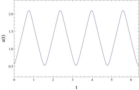
Figure 1: Numerical solution for the scale factor of the universe, governed by Eqs. (5) and (6), for the rescaled choices of parameters $\beta=3(1+w_{d})=-6.6$, $\rho_{0}/\rho_{\rm crit}=0.005$, $a_{i}=0.56$ and $\dot{a}(0)=1$. This shows an oscillatory behaviour for the scale factor in the whole evolution of the universe.

III Quantum field theory

We consider the cyclic cosmological background, resulted from LQC, which was presented in the previous section. In this section, we study the propagation of quantum fields on this background space-time. Then, we investigate circumstances for creation of quantum particles near the future bounce.

III.1 Scalar field on the quantum corrected FLRW background space-time

Let us consider a real (inhomogeneous) scalar field $\phi(t,\vec{x})$ on a FLRW background, whose Lagrangian is

$$\mathcal{L}_{\phi}\ =\ -\frac{1}{2}\left(g^{ab}\partial_{a}\phi\partial_{b}\phi+m^{2}\phi^{2}+\xi{\cal R}\phi^{2}\right),$$ (16)

where ${\cal R}$ is the curvature of the gravitational system; the coupling constants $\xi=0$ and $\xi=1/6$ denote respectively, to the cases of minimally and non-minimally coupled scalar fields. By variation of the Lagrangian above with respect to $\phi$, we obtain the Klein-Gordon equation

$$\left(\square-m^{2}-\xi{\cal R}\right)\phi(t,\vec{x})\ =\ 0\ .$$ (17)

Performing the Legendre transformation, one gets the canonically conjugate momentum for the test field $\phi$, denoted by $\pi_{\phi}$, on a $t=const$ slice. Then, for the pair $(\phi,\pi_{\phi})$, the classical solutions of the equation of motion (coming from (16)) can be expanded in Fourier modes:

$$\phi(t,\vec{x})\ =\ \frac{1}{(2\pi)^{\frac{3}{2}}}\int d^{3}k~{}\phi_{\vec{k}}(t)e^{i\vec{k}\cdot\vec{x}},$$ (18)

$$\pi_{\phi}(t,\vec{x})\ =\ \frac{1}{(2\pi)^{\frac{3}{2}}}\int d^{3}k~{}\pi_{\vec{k}}(t)e^{i\vec{k}\cdot\vec{x}},$$ (19)

where the Fourier coefficients $\phi_{\vec{k}}(t)$ and $\pi_{\vec{k}}(t)$ satisfy the commutation relation $\{\phi_{\vec{k}},\pi_{\vec{k}^{\prime}}\}=\delta(\vec{k}+\vec{k}^{\prime})$, and the reality conditions $\phi_{\vec{k}}^{\ast}=\phi_{-\vec{k}}$ and $\pi_{\vec{k}}^{\ast}=\pi_{-\vec{k}}$ mw .

In the conformal form, the FLRW metric reads

$$g_{ab}dx^{a}dx^{b}\ =\ C(\eta)\left(-d\eta^{2}+d\vec{x}^{2}\right)\ ,$$ (20)

with $\eta$ being the conformal time where $C^{1/2}(\eta)d\eta=dt$. For convenience, we introduce the auxiliary field given by $\chi:=a\phi$, so that, each mode of the form $\phi_{\vec{k}}:=\chi_{\vec{k}}/a$ satisfies the equation

$$\chi_{\vec{k}}^{\prime\prime}+\Omega_{k}^{2}(\eta)\chi_{\vec{k}}=0\ .$$ (21)

A ‘prime’ denotes to the derivative with respect to the conformal time $\eta$. The frequency $\Omega_{k}$ is given by Birrell

$$\Omega_{k}^{2}(\eta)\ :=\ k^{2}+C(\eta)\left[m^{2}+(\xi-1/6){\cal R}\right]\ ,$$ (22)

where $k^{2}=|\vec{k}|^{2}$, and ${\cal R}(\eta)=3(C^{\prime\prime}/C^{2}-C^{\prime 2}/C^{3})$; for the case $C(\eta)=a^{2}(\eta)$ the curvature reads ${\cal R}=6(a^{\prime\prime}/a^{3})$. The normalization condition for $\chi_{\vec{k}}$ is given by mw

$$W(\chi_{\vec{k}}^{*},\chi_{\vec{k}})\ =\ \chi_{\vec{k}}\chi_{\vec{k}}^{*\prime}-\chi_{\vec{k}}^{*}\chi_{\vec{k}}^{\prime}\ =\ 2i\ .$$ (23)

The functions $\chi_{\vec{k}}$ satisfy the initial conditions at a particular moment of time $\eta_{i}$, being the preferred mode functions which determine the (initial) vacuum state, or the lowest energy state.

In this paper, we will consider a non-minimal coupling scalar field, i.e., $\xi=1/6$. In this case, the frequency (22) reduces to

$$\Omega_{k}^{2}(\eta)\ =\ k^{2}+m^{2}a^{2}(\eta)\ .$$ (24)

In order to find the evolution of quantum fields in our cosmological background in all times, we need to consider both cosmological regions (i.e., $0<t<t_{0}$ and $t_{0}<t<t_{b}$) as described in section II.

It is difficult to solve the Klein-Gordon equation (21) for the general forms (9) and (13) of the scale factor, so that we will consider some simplifications. To do that, we first divide the entire evolution of the universe into two phases: one which characterizes the “primordial bounce” phase ($t\rightarrow 0$), for which it is possible to solve the Klein-Gordon equation, so that, the solution naturally contains the structure of the vacuum state of quantum fields (say, the ‘in’ region). The other which characterizes the “late time bounce” phase ($t\rightarrow t_{b}$). Then, we will investigate the possibility of the particle creation at the late time bounce (i.e., the ‘out’ region).

1. In the ‘primordial phase’, close to the initial bounce where $t\rightarrow 0$, one may expand the general expression of the scale factor (9) as

   $$a(t)\ =\ a_{i}\left(1+s^{2}t^{2}\right)+{\cal O}(t^{4})\ ,$$ (25)

   where $s^{2}:=\kappa\rho_{\rm crit}/4$. In terms of the conformal time $\eta$, by using the relation $a^{-1}dt=d\eta$, we can rewrite the scale factor (25) as

   $$a(\eta)\ \approx\ a_{i}\sec^{2}\left(sa_{i}\eta\right)\ .$$ (26)

   This indicates that as $t\rightarrow 0$, then $\eta\rightarrow\eta_{i}=0$ at the initial bounce; $a(\eta_{i}=0)=a_{i}$. Then, for small $\eta$, close to the initial bounce, we can expand Eq. (26) and take the first order terms:

   $$a(\eta)\ \approx\ a_{i}+s^{2}a_{i}^{3}\eta^{2}\ ,$$ (27)

   from which we have (to the first order terms)

   $$\Omega_{k}^{2}(\eta)\ \approx\ \omega_{i}^{2}+2m^{2}a_{i}^{4}s^{2}\eta^{2}\ .$$ (28)

   where $\omega_{i}^{2}:=k^{2}+m^{2}a_{i}^{2}$. For later convenience, let us define new variables $x:=\sqrt{2\sqrt{2}ms}a_{i}\eta$ and $\tilde{\omega}_{i}^{2}=\omega_{i}^{2}/2\sqrt{2}msa_{i}^{2}$; in terms of these variables, we rewrite the Kelin-Gordon equation (21) for the frequency (28) as

   $$\frac{\partial^{2}\chi_{\vec{k}}}{\partial x^{2}}+\left(\tilde{\omega}_{i}^{2}+\frac{x^{2}}{4}\right)\chi_{\vec{k}}(x)=0\ .$$ (29)

   This equation presents a parabolic cylinder equation whose solution can be written as a combination of hypergeometric functions ${}_{1}F_{1}(p,q,ix^{2}/2)$ Handbook :

   $$\quad\quad\chi_{\vec{k}}(x)\ =\ e^{-i\frac{x^{2}}{4}}\left[c_{1}~{}_{1}F_{1}\left(p_{1},q_{1},ix^{2}/2\right)\right.$$

   $$\ \quad\quad\quad\left.+c_{2}x~{}_{1}F_{1}\left(p_{2},q_{2},ix^{2}/2\right)\right],$$ (30)

   where $c_{1,2}$ are constants, $p_{1}=(i\tilde{\omega}_{i}^{2}/2+1/4)$,  $q_{1}=1/2$; and $p_{2}=(i\tilde{\omega}_{i}^{2}/2+3/4)$,  $q_{2}=3/2$. Let us rewrite the solution (30) in the form

   $$\quad\chi_{\vec{k}}(x)\ =\ c_{1}\chi_{\vec{k}}^{(1)}(x)+c_{2}\chi_{\vec{k}}^{(2)}(x)\ .$$ (31)

   Then, by expanding the hypergeometric functions ${}_{1}F_{1}(p,q,ix^{2}/2)$ as series Handbook , we obtain

   $$\quad\quad\chi_{\vec{k}}^{(1)}=1-\tilde{\omega}_{i}^{2}\frac{x^{2}}{2!}-\left(\frac{1}{2}-\tilde{\omega}_{i}^{4}\right)\frac{x^{4}}{4!}+\cdot\cdot\cdot$$ (32)

   $$\quad\quad\chi_{\vec{k}}^{(2)}=x-\tilde{\omega}_{i}^{2}\frac{x^{3}}{3!}-\left(\frac{3}{2}-\tilde{\omega}_{i}^{4}\right)\frac{x^{5}}{5!}+\cdot\cdot\cdot$$ (33)

   Considering only to the order $x^{3}$ for odd series (and $x^{2}$ for even series), Eq. (31) reduces to

   $$\quad\chi_{\vec{k}}(x)\ \approx\ c_{1}\cos(\tilde{\omega}_{i}x)+\frac{c_{2}}{\tilde{\omega}_{i}}\sin(\tilde{\omega}_{i}x)\ .$$ (34)

   By choosing $c_{1}=1/\sqrt{2\omega_{i}}$ and $c_{2}=i\tilde{\omega}_{i}/\sqrt{2\omega_{i}}$, we can rewrite (34), in terms of the conformal time $\eta$, as a typical normalized quantum vacuum state:

   $$\quad\chi_{\vec{k}}(\eta)\ =\ \frac{1}{\sqrt{2\omega_{i}}}e^{i\omega_{i}\eta}\ ,$$ (35)

   which is in fact the initial vacuum state at $\eta\rightarrow\eta_{i}=0$. Moreover, with the same choices of $c_{1,2}$ in Eq. (30) we have the solution for the quantum modes at any time. Notice that, the modes (35) are the negative-frequency solution with respect to $\eta$, therefore, all modes with equal $\omega_{i}$ are complex solutions of Eq. (21) such that, for a chosen mode function $v_{k}(\eta)$ of that equation, the general solution $\chi_{\vec{k}}(\eta)$ can be expressed as Birrell

   $$\quad\quad\chi_{\vec{k}}(\eta)\ =\ \frac{1}{\sqrt{2}}\left[A_{\vec{k}}^{-}v_{k}(\eta)+A_{-\vec{k}}^{+}v_{k}^{\ast}(\eta)\right]\ ,$$ (36)

   where $A_{\vec{k}}^{\pm}$ are constants of integration (being the so-called “annihilation” and “creation” operators with respect to the mode $\chi_{\vec{k}}$ in quantum theory), and the mode function $v_{k}(\eta)$ is given by

   $$v_{k}(\eta)\ =\ \frac{1}{\sqrt{\omega_{i}}}e^{-i\omega_{i}\eta}\ ,$$ (37)

   which is normalized due to $W[v_{k},v_{k}^{\ast}]=2i$ given in Eq. (23). Imposing the reality condition $\chi_{\vec{k}}^{\ast}(\eta)=\chi_{-\vec{k}}(\eta)$ into Eq. (36) we get $A_{\vec{k}}^{+}=(A_{\vec{k}}^{-})^{\ast}$; then by using Fourier series we can express the expansion of $\chi(\eta,\vec{x})$ as

   $$\chi(\eta,\vec{x})\ =\ \frac{1}{(2\pi)^{\frac{3}{2}}}\int d^{3}k~{}\chi_{\vec{k}}(\eta,\vec{x})\ ,$$ (38)

   where $\chi_{\vec{k}}(\eta,\vec{x})$ is given by

   $$\quad\quad\chi_{\vec{k}}(\eta,\vec{x})=A_{\vec{k}}^{-}\frac{v_{k}(\eta)}{\sqrt{2}}e^{i\vec{k}\cdot\vec{x}}+A_{\vec{k}}^{+}\frac{v_{k}^{\ast}(\eta)}{\sqrt{2}}e^{-i\vec{k}\cdot\vec{x}}.$$ (39)

   In the summation above we have changed the variables as $\vec{k}\rightarrow-\vec{k}$.

2. At the ‘late time phase’ as $t\rightarrow t_{b}$, the scale factor (13) can be approximated as

   $$\quad\quad\bar{a}(\tau)\ =\ a_{b}\left(1-\tilde{s}^{2}\tau^{2}\right)+{\cal O}\big{(}\tau^{4}\big{)}\ ,$$ (40)

   where $\tau:=t-t_{b}$ and $\tilde{s}^{2}:=\frac{\kappa}{12}\rho_{\rm crit}|\beta|$. Replacing $\bar{a}(t)$ in $\bar{a}d\tau=d\eta$ from Eq. (40), by integration we obtain the scale factor in terms of the proper time:

   $$\bar{a}(\eta)\ \approx\ a_{b}-\tilde{s}^{2}a_{b}^{3}(\eta-\eta_{b})^{2}\ ,$$ (41)

   where $\eta_{b}$ is the proper time at which the universe hits a bounce at late time. The Eq. (41) looks like the primordial scale factor (27), so that, with a similar analysis we obtain the scalar field as solution to Klein-Gordon equation. In particular, for (41) the frequency (when considering only first order terms) reads

   $$\quad\Omega_{k}^{2}(\eta)\ \approx\ \omega_{b}^{2}-2m^{2}a_{b}^{4}\tilde{s}^{2}(\eta-\eta_{b})^{2}\ .$$ (42)

   where $\omega_{b}^{2}:=k^{2}+m^{2}a_{b}^{2}$. By introducing $y:=\sqrt{2\sqrt{2}m\tilde{s}}a_{b}(\eta-\eta_{b})$, the Klein-Gordon equation for the frequency (42), in terms of new variable reads

   $$\frac{\partial^{2}\chi_{\vec{k}}}{\partial y^{2}}-\left(\frac{y^{2}}{4}-\tilde{\omega}_{b}^{2}\right)\chi_{\vec{k}}(y)=0\ ,$$ (43)

   where $\tilde{\omega}_{b}^{2}:=\omega_{b}^{2}/2\sqrt{2}m\tilde{s}a_{b}^{2}$. The differential equation (43), as before, is a parabolic cylinder equation whose solutions can be expressed as Handbook

   $$\quad\quad\chi_{\vec{k}}^{(1)}=1-\tilde{\omega}_{b}^{2}\frac{y^{2}}{2!}+\left(\frac{1}{2}+\tilde{\omega}_{b}^{4}\right)\frac{y^{4}}{4!}+\cdot\cdot\cdot$$ (44)

   $$\quad\quad\chi_{\vec{k}}^{(2)}=y-\tilde{\omega}_{b}^{2}\frac{y^{3}}{3!}+\left(\frac{3}{2}+\tilde{\omega}_{b}^{4}\right)\frac{y^{5}}{5!}+\cdot\cdot\cdot$$ (45)

   Taking only the orders $x^{3}$ for odd series and $x^{2}$ for even series, we express the total solution to (43) as a combination of (44) and (45):

   $$\quad\chi_{\vec{k}}(y)\ \approx\ \tilde{c}_{1}\cos(\tilde{\omega}_{b}y)+\frac{\tilde{c}_{2}}{\tilde{\omega}_{b}}\sin(\tilde{\omega}_{b}y)\ ,$$ (46)

   for arbitrary constants of integration $\tilde{c}_{1}$ and $\tilde{c}_{2}$. For the choices of $\tilde{c}_{1}=1/\sqrt{2\omega_{b}}$ and $\tilde{c}_{2}=i\tilde{\omega}_{b}/\sqrt{2\omega_{b}}$, Eq. (46) reduces to $\chi_{\vec{k}}(\eta)\sim e^{i\omega_{b}(\eta-\eta_{b})}/\sqrt{2\omega_{b}}$, indicating a (negative-frequency solution) vacuum state at late time (i.e., the ‘out’ region).

   For each mode, the general solution to the Klein-Gordon equation (21), in terms of the mode function $u_{k}(\eta)$ of the ‘out’ vacuum, can be expanded, by using the new Bogolyubov coefficients as Birrell

   $$\quad\quad\chi_{\vec{k}}(\eta)\ =\ \frac{1}{\sqrt{2}}\left[B_{\vec{k}}^{-}u_{k}(\eta)+B_{-\vec{k}}^{+}u_{k}^{\ast}(\eta)\right]\ ,$$ (47)

   in which a new complete orthonormal set of (positive-frequency) modes $u_{k}$ was considered as

   $$u_{k}(\eta)\ =\ \frac{1}{\sqrt{\omega_{b}}}e^{-i\omega_{b}(\eta-\eta_{b})}\ .$$ (48)

   Notice that, similar to the ‘in’ region in the primordial phase, $u_{k}(\eta)$ herein this phase, defines the final vacuum state in the ‘out’ region as $\eta\rightarrow\eta_{b}$. The $B_{\vec{k}}^{\pm}$ are constants of integration; similarly they are the annihilation and creation operators in quantum theory, but, with respect to the new vacuum state $u_{k}(\eta)$. Therefore, similar to (39) we can express the solution $\chi_{\vec{k}}(\eta,\vec{x})$ as

   $$\quad\quad\chi_{\vec{k}}(\eta,\vec{x})=B_{\vec{k}}^{-}\frac{u_{k}(\eta)}{\sqrt{2}}e^{i\vec{k}\cdot\vec{x}}+B_{\vec{k}}^{+}\frac{u_{k}^{\ast}(\eta)}{\sqrt{2}}e^{-i\vec{k}\cdot\vec{x}},$$ (49)

   where we again applied $\vec{k}\rightarrow-\vec{k}$ in the second term.

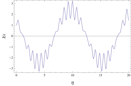
Figure 2: Time evolution of the quantum field mode $\chi_{k}(\eta)$, given by the Klein-Gordon equation (21), evolving between the initial and final bounces. We considered the following rescaled choices of parameters in our numerical analysis: $\beta=3(1+w_{d})=-6.6$, $\rho_{0}/\rho_{\rm crit}=0.005$, $a_{i}=0.56$, $\dot{a}(0)=\dot{a}_{i}=1$, $k=0.5$ and $m=0.001$ in Planck units.

Figure 2 shows typical numerical solution to the Klein-Gordon equation (21) for the field in the herein cyclic cosmological model, for sub-planckian values of the mass $m$ and wavenumbers $k$. It presents an oscillatory behaviour for scalar field evolving in the universe between the initial and final bounces. When those parameters become trans-planckians, the oscillations give places to asymptotically divergent behaviour, as could be expected.

Frequencies (28) and (42) are the same for a massless field, thus, the solutions (39) and (49) can be written in the form of the plane waves in two phases. Since the solutions must be continuous, there is no final effect in the final bouncing phase for particle production. However, in the massive case situation is totally different. In order to discuss this more precisely, we will calculate, in the following section, the Bogolyubov coefficients at the final bounce in the presence of non-unique vacuum solutions in the ‘in’ and ‘out’ regions.

III.2 The Bogolyubov transformations

In quantum theory, the mode operator $\hat{\chi}_{\vec{k}}(\eta,\vec{x})$ can be expressed through the creation and annihilation operators Birrell : in the primordial phase, where $\eta\rightarrow 0$ (denoted by ‘in’ region), constants $A_{\vec{k}}^{\pm}$ are denoted to be the annihilation and creation operators. Thus, replacing this in Eq. (39) we obtain the mode operators:

$$\hat{\chi}_{\vec{k}}^{\rm(in)}(\eta,\vec{x})=\hat{A}_{\vec{k}}^{-}\frac{v_{k}(\eta)}{\sqrt{2}}e^{i\vec{k}\cdot\vec{x}}+\hat{A}_{\vec{k}}^{+}\frac{v_{k}^{\ast}(\eta)}{\sqrt{2}}e^{-i\vec{k}\cdot\vec{x}}.$$ (50)

Similarly, for the late time bounce phase, where $\eta\rightarrow\eta_{b}$ (denoted by ‘out’ region), from Eq. (49) we obtain the mode operators as

$$\hat{\chi}_{\vec{k}}^{\rm(out)}(\eta,\vec{x})=\hat{B}_{\vec{k}}^{-}\frac{u_{k}(\eta)}{\sqrt{2}}e^{i\vec{k}\cdot\vec{x}}+\hat{B}_{\vec{k}}^{+}\frac{u_{k}^{\ast}(\eta)}{\sqrt{2}}e^{-i\vec{k}\cdot\vec{x}}.$$ (51)

The expansions (50) and (51) express the same field $\hat{\chi}_{\vec{k}}(\eta,\vec{x})$ through two different sets of functions, so the $k$-th Fourier components of these expansions must agree

$$\hat{\chi}_{\vec{k}}^{\rm(in)}(\eta_{c},\vec{x})\ =\ \hat{\chi}_{\vec{k}}^{\rm(out)}(\eta_{c},\vec{x})\ ,$$ (52)

at any transition time $\eta=\eta_{c}$. (We can consider $\eta_{c}=\eta_{0}$ to be the transition time from matter dominant region to the dark energy dominant region.) Furthermore, continuity condition at $\eta=\eta_{c}$, from one era to another implies that the (conformal) time derivative of mode functions must satisfy

$$\frac{\partial\hat{\chi}_{\vec{k}}^{\rm(in)}(\eta_{c},\vec{x})}{\partial\eta}\ =\ \frac{\partial\hat{\chi}_{\vec{k}}^{\rm(out)}(\eta_{c},\vec{x})}{\partial\eta}\ .$$ (53)

From the matching conditions (52) and (53) we obtain

$$\hat{B}_{\vec{k}}^{-}\ =\ \alpha_{k}\hat{A}_{\vec{k}}^{-}+\beta_{k}^{\ast}\hat{A}_{-\vec{k}}^{+}\ ,$$ (54)

and

$$\hat{B}_{\vec{k}}^{+}\ =\ \alpha_{k}^{\ast}\hat{A}_{\vec{k}}^{+}+\beta_{k}\hat{A}_{-\vec{k}}^{-}\ .$$ (55)

These relations present the Bogolyubov transformations in which the old annihilation and creation operators $\hat{A}_{\vec{k}}^{\pm}$ are expressed through the new operators $\hat{B}_{\vec{k}}^{\pm}$, with the $\eta$-independent (complex) Bogolyubov coefficients:

$$\alpha_{k}\ =\ \frac{\sqrt{\omega_{b}}}{2\sqrt{\omega_{i}}}\left(1+\frac{\omega_{i}}{\omega_{b}}\right)e^{-i(\omega_{i}-\omega_{b})\eta_{c}-i\omega_{b}\eta_{b}}\ ,$$ (56)

$$\beta_{k}\ =\ \frac{\sqrt{\omega_{b}}}{2\sqrt{\omega_{i}}}\left(1-\frac{\omega_{i}}{\omega_{b}}\right)e^{-i(\omega_{i}+\omega_{b})\eta_{c}+i\omega_{b}\eta_{b}}\ .$$ (57)

Using these coefficients we can express the primordial basis $v_{k}(\eta)$ in terms of the late time one, $u_{k}(\eta)$, as

$$v_{k}(\eta)\ =\ \alpha_{k}u_{k}(\eta)+\beta_{k}u^{\ast}_{k}(\eta)\ .$$ (58)

Since $v_{k}(\eta)$ and $u_{k}(\eta)$ are normalized, it follows that

$$\alpha_{k}\alpha_{k}^{\ast}-\beta_{k}\beta_{k}^{\ast}=1\ .$$ (59)

The coefficient $\beta_{k}$ is associated with the created particles. More precisely, in the Heisenberg picture, the initial vacuum state $|0_{\rm in}\rangle$ in the ‘in’ region is the state of the system for all time. The physical number operator which counts particles in the ‘out’ region reads $\hat{N}_{k}=\hat{B}_{\vec{k}}^{+}\hat{B}_{\vec{k}}^{-}$ Birrell . Then, the mean number of $u_{k}$-mode particles in the state $|0_{\rm in}\rangle$ is given by

$${\cal N}_{k}\ =\ \langle 0_{\rm in}|\hat{N}_{k}|0_{\rm in}\rangle\$$

$$=\ \beta_{k}\beta^{\ast}_{k}\ =\ \frac{\omega_{b}}{4\omega_{i}}\left(1-\frac{\omega_{i}}{\omega_{b}}\right)^{2},$$ (60)

which is to say that the vacuum state of the $v_{k}$ modes contains ${\cal N}_{k}$ particles in the $u_{k}$ mode. For a massless scalar field, $\omega_{i}=\omega_{b}=|\vec{k}|$, thus, $\alpha_{k}=1$, $\beta_{k}=0$ and the mean density ${\cal N}_{k}$ is zero; therefore, no particle is produced in the case of a massless scalar field in the ‘out’ region.

III.3 The energy density of created particles

The relation (60) is the average number of late time particles per spatial volume and per wave number $k$. The energy density of the $\ell$ particles in the vacuum state $|0_{\rm in}\rangle$ for each mode $v_{k}$ reads $\rho_{k}=(\frac{1}{2}+\ell)\omega_{i}$, where $w_{i}/2$ is the zero-point energy. Since the chosen quantum state corresponds to the ‘in’ vacuum $|0_{\rm in}\rangle$, then in the ‘out’ region ($\eta\rightarrow\eta_{b}$) the combined mean density of total particles for each mode $k$ (after subtracting the zero-point energy) is $\rho_{k}={\cal N}_{k}\omega_{i}$ Birrell:1980 . Then, for all modes (per unit volume), we obtain the density of late time particles as

$$\rho_{P}\ =\ \int_{0}^{\infty}\frac{d^{3}k}{(2\pi)^{3}}|\beta_{k}|^{2}\omega_{i}$$

$$=\ \int_{0}^{\infty}\frac{dk}{8\pi^{2}}~{}k^{2}\omega_{b}\left(1-\frac{\omega_{i}}{\omega_{b}}\right)^{2}\ .$$ (61)

At small scales close to the initial bounce (‘in’ region) we can approximate $ma_{i}\ll 1$, thus, $\omega_{i}\approx k$. Then, Eq. (61) reduces to

$$\rho_{P}\ \approx\ \frac{1}{8\pi^{2}}\int dk~{}k^{2}\omega_{b}\left(1-\frac{k}{\omega_{b}}\right)^{2}$$

$$=\ \frac{1}{8\pi^{2}}\left[\omega_{b}k\left(\frac{k^{2}}{2}-\frac{m^{2}a_{b}^{2}}{4}\right)\right.$$

$$\quad\quad\quad\quad\left.-\frac{k^{4}}{2}+\frac{m^{2}a_{b}^{2}}{4}\ln(2k+2\omega_{b})\right].$$ (62)

This integral has obviously, a logarithmic divergence when it tends to the ultraviolet limit, $k\rightarrow\infty$ Julio:2008 ; Julio:2011 , so that it is necessary to regularize it.

Using the $n$-wave method developed in Ref. Pauli-Villars , which consists in subtracting terms obtained by expanding $\rho_{k}$ in powers of $k^{-2}$:

$$\rho_{k}^{\rm ren}\ =\ \rho_{k}-E_{k}^{(0)}-E_{k}^{(1)}-\frac{1}{2}E_{k}^{(2)}$$ (63)

in which we have defined

$$E^{(p)}_{k}\ =\ \lim_{n\rightarrow\infty}\frac{\partial^{p}\rho_{k}^{(n)}}{\partial(n^{-2})^{p}}\ ,$$ (64)

where $\rho_{k}^{(n)}:=\rho_{k}(nk,nm)/n$, and $n$ is the parameter that characterizes the order of the divergence. Therefore, $E_{k}^{(0)}$, $E_{k}^{(1)}$ and $E_{k}^{(2)}$ eliminate, respectively, the logarithmic, quadratic and the quartic divergences. Following the regularisation procedure corresponding to a full renormalisation of the coupling constants Grib:1994 ; Grib:1998 , we have that

$$\rho_{k}\ =\ \omega_{b}-2k+\frac{k^{2}}{\omega_{b}}$$ (65)

which follows that $\rho_{k}^{(n)}=\rho_{k}$; then, we find the renormalised energy as Julio:2011

$$\rho_{k}^{\rm ren}\ =\ \rho_{k}-E^{0}_{k}\ =\ 0\ ,$$ (66)

which is zero. Vanishing energy density of created particles indicate that quantum field effects associated with the cosmological dynamics at late time do not change the nature of quantum gravity bounce in the far future.

IV Conclusion and Discussion

In this work, we considered a flat FLRW universe whose matter content is dominated by a dust fluid at early time and a phantom dark energy component at late time (cf. see Section II). We employed loop quantum cosmology to govern the geometry of space-time at Planck era. In particular, quantum gravity effects modified the dynamics of the universe in the primordial and late time phases, thus, resolved the big bang singularity in the past and the big rip singularity in the future, and replaced them by quantum bounces. This indicated that the resulting quantum bounce and recollapse in our herein model contribute a cyclic scenario for the universe. In classical cosmology, in general, different matter components provide different types of singular fate for the universe at late times. Subsequently, loop quantum gravity resolves those singularities so that the resulting quantum bounce and recollapse give rise to different cyclic scenarios for the universe. Our main concern in this paper was to construct a cyclic scenario in the FLRW universe, in order to investigate the phenomena of cosmological particle production by quantum gravity effects. Nevertheless, for further studies of possible cyclic models driven by loop quantum cosmology, we suggest readers to refer to the recent paper Ref. Singh:2011 and references therein.

We studied quantum theory of a massive, non-minimally coupled scalar field on the resulting cyclic cosmological background. Our aim was to investigate particle production by semiclassical gravitational effects, in an expanding phase towards late time. In general, in a curved space-time background, it is not possible to define a unique vacuum state Parker:1974 . However, in the asymptotically static ‘in’ or ‘out’ regions followed by a period of expansion, the notion of asymptotic vacuum states come closest to a Minkowski-like vacuum Birrell . In our herein model, the scale factor of the universe starts expanding from an initial quantum bounce (for some times $\eta_{i}\sim 0$, on $a\sim a_{i}$, where $a_{i}\sim(M/m_{\rm Pl})^{1/3}\ell_{\rm Pl}$ and $M$ is the total mass of the universe) towards a late time bounce (for some times $\eta\sim\eta_{b}$, where $a\sim a_{b}=a_{0}(\rho_{\rm crit}/\rho_{0})^{1/|\beta|}$). Therefore, the scale factor of the universe admits two asymptotic static forms at the initial and final states. We have used this static approximation, as ‘in’ or ‘out’ regions, in the computation of created particles (cf. Section III). However, it must be stressed that, this does not lead to a trivial situation, since this approximation is different from the usual Minkowski asymptotic approximation Birrell and from the sudden singularity approximation Julio:2008 ; Julio:2011 : in the present case, the transition from a matter dominated region to a dark energy dominated region, gave rise to the Planck regimes (in which quantum gravity effects are inevitable) at two different asymptotic phases, which consequently, leaded to distinct ‘in’ and ‘out’ vacuum states. Moreover, in the asymptotic limits (i.e., $\eta\rightarrow 0$ and $\eta\rightarrow\eta_{b}$), the first time derivative of the scale factor is zero, but the second time derivative is finite. These different contexts are reflected in the matching conditions (via transition time $\eta_{c}$) connecting the initial and final states. Nevertheless, it does not affects on the final particle production, since the particle number (cf. see Eq. (60)) depends only on the characteristic of the initial and final vacuum.

For a scalar field, undergoing cosmological evolution between the initial and final static phases, we solved the Klein-Gordon equation in the (past) matter dominated region ($\eta<\eta_{0}$), and the (future) dark energy dominated region ($\eta>\eta_{0}$); the conformal time $\eta_{0}$ denotes the present, being the transition time (i.e., $\eta_{c}=\eta_{0}$) from matter dominated regime to dark energy dominated regime. We obtained mode functions of the fields close to the initial and final bounces whose forms are similar to that of a flat space mode function. For the herein massive scalar field, different cosmic scales of the initial and final phases leaded to different frequencies for the modes of the quantum fields, and consequently, provided non-unique vacuum states in the ‘in’ and ‘out’ regions; this non-uniqueness of the vacuum was accompanied by particle production phenomena in the ‘out’ region. For a massless scalar field, however, mode functions of the ‘in’ and ‘out’ regions are the same as $e^{-ik\eta}$, possessing a unique vacuum of the Minkowski space; hence, there is no final effects for the particle production at late time, for massless fields.

The energy density of quantum scalar field, $\rho_{\varphi}$, in the herein model, was assumed to be negligible initially in comparison to the quantum background density (which is of the order $\rho\sim\rho_{\rm crit}=0.41\rho_{\rm Pl}$) near the initial bounce. Moreover, there were no particles production initially since $A_{\vec{k}}^{+}A_{\vec{k}}^{-}|0_{\rm in}\rangle=0$. Our concern, thus, was to investigate the back-reaction of quantum effects carried by the total particles created in the ‘out’ region. We thus computed the total density of the quantum particles, $\rho_{P}$, created at late time, on approach to the future bounce where the energy density, curvature and the scale factor of the background geometry reaches their upper bounds. Our analysis showed that the density of created particles in the ‘out’ region remains negligible in comparison to the quantum background density (i.e, $\rho_{P}\ll\rho_{\rm crit}$). This indicates that the back-reaction effects of the quantum particle production do not influence the evolution of the universe until late time. In addition, the future bounce, induced by quantum gravity effects, was unscathed by the back-reaction from the quantum field.

One important issue for the model analysed here is the possibility of observational traces of the quantum phase and of the oscillatory behaviour of the universe. This would require, for example, to compute the evolution of perturbations in the model. However, we must face an important limitation: We have no classical covariant formulation of the equations of motion governing the evolution of the universe. Strictly speaking, this analysis would require to return to the full quantum model in performing the perturbative analysis, what implies in considerable technical difficulties (c.f. Refs. Ashtekar:2013 ; Andrea:2013 ). This drawback is less severe in the case of gravitational waves (see Ref. Bojowald:GW ), since there is no coupling of the spin 2 modes with the scalar and vectorial modes (which are directly connected to the matter content), at least at linear level. If the gravitational waves, represented by the propagation of the traceless, transverse field $\delta g_{ij}=h_{ij}$, obeys the same equation as in the usual general relativity case, that is,

$$\mu^{\prime\prime}+\Big{(}k^{2}-\frac{a^{\prime\prime}}{a}\Big{)}\mu\ =\ 0,$$ (67)

where $h_{ij}=a\epsilon_{ij}\mu$, with $\epsilon_{ij}$ being the polarisation tensor and $a(\eta)$ the scale factor, we would have the same equation as for a massless scalar field propagating in the geometry determined by the background equations Grishchuk:1993 . We would have in this case, qualitatively, the same behaviour as displayed in figure 2 for the massive field, but with an accumulative divergence for transplackian values of $k$. However, it is not sure that equation (67) remains the same in the present case. Moreover, the transplanckian regime would require a full quantum analysis, including for the background. Due to these important difficulties to surmount, we postpone a perturbative analysis for future researches.

In general, a cyclic universe seems to be in conflict with the second law of thermodynamics. More precisely, the entropy of the universe increases, through natural thermodynamic processes, in every cycle of expansion and contraction Tolman:1931 ; Tolman:1934 . So that, at the beginning of a new cycle, there is higher entropy density (than the previous cycle) because of the entropy added from earlier cycles. It turns out that the duration of a cycle is sensitive to the entropy density, thus by increasing the entropy, the duration of the cycle increases as well. On the other hand, the cycles become shorter and shorter the further back we go until, after a finite time, they shrink to zero duration. New hope for a consistent cyclic cosmology, to get rid of this puzzling situation, was provided by introducing a cyclic model based on (phantom) dark energy Baum-Frampton:2007 ; Baum-Frampton:2008 , and also in an ekpyrotic scenario derived from the brane-world cosmological model Steinhardt-Turok : in both scenarios, there are accelerating phases leading to a suppression of entropy. In the context of LQC, there are several proposals in order to deal with the issue of entropy problem in bouncing universe Bojowald:2007 ; Bojowald:2008 ; Corichi:2008 . In addition, presence of the quantum fields in such bouncing scenario may also give rise to the significant effects on entropy generation from particle creation; there are inquiries on finding a viable measure of entropy for particle production processes in literature (see for example Refs. Hu:1986 ; Hu:1987 ). In the present model, the oscillatory behaviour indicated in the quantum modes (see figure 2) may be a hint that there is no major problem with the cumulative effects as the cycle goes on. This oscillatory behaviour breaks down as the Planck regime is approached. But, the approximation made in the present work may not be valid in the deep Planck regime. The necessary renormalization procedure changes also the high frequency behaviour. Nevertheless, more investigation is needed in order to understand the effects of particle creation on generation of the entropy near the quantum bounce in the full quantum theory.

References

- (1) N. D. Birrell and P. C. W. Davies, Quantum Fields in Curved Space, (Cambridge University Press 1982).
- (2) V. Mukhanov and S. Winitzki, Introduction to Quantum Effects in Gravity, (Cambridge University Press, Cambridge, 2007)
- (3) S. A. Fulling, Aspects of Quantum Field Theory in Curved Spacetime, (Cambridge Univ. Press, Cambridge, 1989).
- (4) A. Ashtekar and J. Lewandowski, Background independent quantum gravity: A status report, Class. Quant. Grav. 21, R53-R152 (2004).
- (5) C. Rovelli,Quantum Gravity (Cambridge University Press, Cambridge (2004)).
- (6) T. Thiemann, Introduction to Modern Canonical Quantum General Relativity, (Cambridge University Press, Cambridge, (2007)).
- (7) A. Ashtekar, M. Bojowald and J. Lewandowski, Mathematical structure of loop quantum cosmology. Adv. Theo. Math. Phys. 7, 233–268 (2003).
- (8) A. Ashtekar, Loop Quantum Cosmology: An Overview (2007), Gen. Rel. and Grav. (at Press), [arXiv: gr-qc/0812.0177].
- (9) M. Bojowald, Loop quantum cosmology, Liv. Rev. Rel. 11, 4 (2008).
- (10) M. Bojowald, Quantum Cosmology: A Fundamental Description of the Universe (Lecture Notes in Physics), (Springer, 2011).
- (11) A. Ashtekar, P. Singh, Loop Quantum Cosmology: A Status Report, Class. Quant. Grav. 28: 213001 (2011).
- (12) A. Ashtekar, T. Pawlowski and P. Singh, Quantum nature of the big bang, Phys. Rev. Lett. 96, 141301 (2006).
- (13) A. Ashtekar, T. Pawlowski and P. Singh, Quantum nature of the big bang: An analytical and numerical investigation I, Phys. Rev. D 73, 124038 (2006).
- (14) A. Ashtekar, T. Pawlowski and P. Singh, Quantum nature of the big bang: Improved dynamics, Phys. Rev. D 74, 084003 (2006).
- (15) M. Sami, P. Singh, S. Tsujikawa, Avoidance of future singularities in loop quantum cosmology Phys. Rev. D 74, 043514 (2006).
- (16) P. Singh, F. Vidotto, Exotic singularities and spatially curved Loop Quantum Cosmology, Phys. Rev. D 83, 064027 (2011).
- (17) Y. Ding, Y. Ma, and J. Yang, Effective Scenario of Loop Quantum Cosmology, Phys. Rev. Lett. 102, 051301 (2009).
- (18) P. A. R. Ade, et al., [Planck Collaboration] Planck 2013 results. XVI. Cosmological parameters, Astron. Astrophys. 571, 66 (2014); [arXiv: 1303.5076 [astro-ph.CO]].
- (19) A. A. Starobinsky, Future and origin of our Universe: modern view, Grav. Cosmol. 6, 157 (2000), [arXiv: astro-ph/9912054]; B. McInnes, The dS/CFT Correspondence and the Big Smash, JHEP 0208, 029 (2002); R. R. Caldwell, M. Kamionkowski and N. N. Weinberg, Phantom Energy and Cosmic Doomsday, Phys. Rev. Lett. 91, 071301 (2003), [arXiv: astro-ph/0302506].
- (20) A. Ashtekar, W. Kaminski and J. Lewandowski, Quantum field theory on a cosmological, quantum space-time Phys.Rev. D 79, 0644030 (2009).
- (21) A. Dapor, J. Lewandowski, and Y. Tavakoli, Lorentz Symmetry in QFT on Quantum Bianchi I Space-Time, Phys. Rev. D 86, 064013 (2012).
- (22) I. Agullo, A. Ashtekar, W. Nelson, Extension of the quantum theory of cosmological perturbations to the Planck era, Phys. Rev. D 87, 043507 (2013).
- (23) A. Dapor, J. Lewandowski, J. Puchta, QFT on quantum space-time: a compatible classical framework, Phys. Rev. D 87, 104038 (2013).
- (24) L. Parker, The creation of particles in an expanding universe, PhD thesis (Harvard University, 1966).
- (25) L. Parker, Quantized Fields and Particle Creation in Expanding Universes. I, Phys. Rev. 183, 1057 (1969); Quantized Fields and Particle Creation in Expanding Universes. II, Phys. Rev. D 3, 346 (1971).
- (26) L. Parker and S. A. Fulling, Adiabatic regularization of the energy-momentum tensor of a quantized field in homogeneous spaces, Phys. Rev. D 9, 341 (1974).
- (27) Ya. B. Zel’dovich and A. A. Starobinsky, Particle Production and Vacuum Polarization in an Anisotropic Gravitational Field, Sov. Phys. JETP 34, 1159 (1972).
- (28) A. A. Grib, S. G. Mamayev and V.M. Mostepanenko, Vacuum quantum effects in strong fields, (Friedmann, St. Petersburg, 1994).
- (29) M. Bordag, J. Lindig and V.M. Mostepanenko, Particle creation and vacuum polarization of a non-conformal scalar field near the isotropic cosmological singularity, Class. Quantum Grav. 15, 581 (1998).
- (30) M. Abramowitz and I. A. Stegun, Handbook of mathematical functions (Dover, New York, 1970), p. 586.
- (31) J. D. Barrow, A. B. Batista, J. C. Fabris, M. J. S. Houndjo and G. Dito, Sudden singularities survive massive quantum particle production, Phys. Rev. D 84, 123518 (2011).
- (32) J. D. Barrow, A. B. Batista, J. C. Fabris and S. Houndjo, Quantum Particle Production at Sudden Singularities, Phys. Rev. D 78, 123508 (2008).
- (33) N. D. Birrell and C. P. W. Davies, Massive particle production in anisotropic space-times, J. Phys. A: Math. Gen. 13, 2109 (1980).
- (34) M. Bojowald, G. M. Hossain, Loop quantum gravity corrections to gravitational wave dispersion, Phys. Rev. D 77, 023508 (2008).
- (35) L. P. Grishchuk, Quantum effects in cosmology, Class. Quantum Grav. 10, 2449-2478 (1993).
- (36) R. C. Tolman, On the problem of entropy of the universe as a whole, Phys. Rev. 37, (1931) 1639–1660.
- (37) R. C. Tolman, Relativity, Thermodynamics and Cosmology, (Clarendon Press, Oxford 1934).
- (38) L. Baum and P. H. Frampton, Turnaround in cyclic cosmology, Phys. Rev. Lett. 98, 071301 (2007).
- (39) L. Baum and P. H. Frampton, Entropy of Contracting Universe in Cyclic Cosmology, Mod. Phys. Lett. A 23, 33 (2008).
- (40) P. J. Steinhardt, N. Turok, Cosmic Evolution in a Cyclic Universe, Phys. Rev. D 65, 126003 (2002).
- (41) M. Bojowald, What happened before the big bang? Nature Physics 3, 523-525 (2007).
- (42) M. Bojowald, R. Tavakol, Recollapsing quantum cosmologies and the question of entropy, Phys. Rev. D 78, 023515 (2008).
- (43) A. Corichi and P. Singh, Quantum bounce and cosmic recall, Phys. Rev. Lett. 100, 162302 (2008).
- (44) B. L. Hu and D. Pavon, Intrinsic measures of field entropy in cosmological particle creation, Phys. Lett. B 180, 329 (1986).
- (45) B. L. Hu and H. E. Kandrup, Entropy generation in cosmological particle creation and interactions: A statistical subdynamics analysis, Phys. Rev. D 35, 1776 (1987).