Feedforward semantic segmentation with zoom-out features

Abstract

We introduce a purely feed-forward architecture for semantic segmentation. We map small image elements (superpixels) to rich feature representations extracted from a sequence of nested regions of increasing extent. These regions are obtained by ”zooming out” from the superpixel all the way to scene-level resolution. This approach exploits statistical structure in the image and in the label space without setting up explicit structured prediction mechanisms, and thus avoids complex and expensive inference. Instead superpixels are classified by a feedforward multilayer network. Our architecture achieves new state of the art performance in semantic segmentation, obtaining 64.4% average accuracy on the PASCAL VOC 2012 test set.

1 Introduction

We consider one of the central vision tasks, semantic segmentation: assigning to each pixel in an image a category-level label. Despite attention it has received, it remains challenging, largely due to complex interactions between neighboring as well as distant image elements, the importance of global context, and the interplay between semantic labeling and instance-level detection. A widely accepted conventional wisdom, followed in much of modern segmentation literature, is that segmentation should be treated as a structured prediction task, which most often means using a random field or structured support vector machine model of considerable complexity.

This in turn brings up severe challenges, among them the intractable nature of inference and learning in many “interesting” models. To alleviate this, many recently proposed methods rely on a pre-processing stage, or a few stages, to produce a manageable number of hypothesized regions, or even complete segmentations, for an image. These are then scored, ranked or combined in a variety of ways.

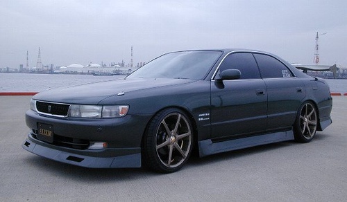
Figure 1: Our feedforward segmentation process. The feature vector for a superpixel consists of components extracted at zoom-out spatial levels: locally at a superpixel (red), in a small proximal neighborhood (cyan), in a larger distant neighborhood (orange), and globally from the entire image (green). The concatenated feature vector is fed to a multi-layer neural network that classifies the superpixel.

Here we consider a departure from these conventions, and approach semantic segmentation as a single-stage classification task, in which each image element (superpixel) is labeled by a feedforward model, based on evidence computed from the image. Surprisingly, in experiments on PASCAL VOC 2012 segmentation benchmark we show that this simple sounding approach leads to results significantly surpassing all previously published ones, advancing the current state of the art from about 52% to 64.4%.

The “secret” behind our method is that the evidence used in the feedforward classification is not computed from a small local region in isolation, but collected from a sequence of levels, obtained by “zooming out” from the close-up view of the superpixel. Starting from the superpixel itself, to a small region surrounding it, to a larger region around it and all the way to the entire image, we compute a rich feature representation at each level and combine all the features before feeding them to a classifier. This allows us to exploit statistical structure in the label space and dependencies between image elements at different resolutions without explicitly encoding these in a complex model.

We should emphasize that we do not mean to dismiss structured prediction or inference, and as we discuss in Section 5, these tools may be complementary to our architecture. In this paper we explore how far we can go without resorting to explicitly structured models.

We use convolutional neural networks (convnets) to extract features from larger zoom-out regions. Convnets, (re)introduced to vision in 2012, have facilitated a dramatic advance in classification, detection, fine-grained recognition and other vision tasks. Segmentation has remained conspicuously left out from this wave of progress; while image classification and detection accuracies on VOC have improved by nearly 50% (relative), segmentation numbers have improved only modestly. A big reason for this is that neural networks are inherently geared for “non-structured” classification and regression, and it is still not clear how they can be harnessed in a structured prediction framework. In this work we propose a way to leverage the power of representations learned by convnets, by framing segmentation as classification and making the structured aspect of it implicit. Last but not least, we show that use of multi-layer neural network trained with asymmetric loss to classify superpixels represented by zoom-out features, leads to significant improvement in segmentation accuracy over simpler models and conventional (symmetric) loss.

Below we give a high-level description of our method, then discuss related work and position our work in its context. Most of the technical details are deferred to Section 4 in which we describe implementation and report on results, before concluding in Section 5.

2 Zoom-out feature fusion

We cast category-level segmentation of an image as classifying a set of superpixels. Since we expect to apply the same classification machine to every superpixel, we would like the nature of the superpixels to be similar, in particular their size. In our experiments we use SLIC [1], but other methods that produce nearly-uniform grid of superpixels might work similarly well. Figures 2 and 3 provide a few illustrative examples for this discussion.

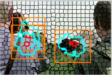
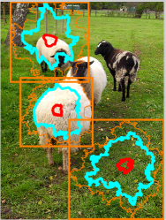
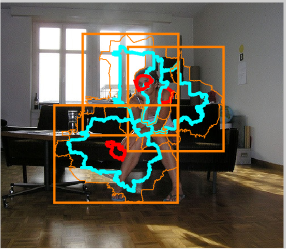
Figure 2: Examples of zoom-out regions: red for superpixel, cyan for proximal region, solid orange for distant region; curved orange line shows the extent of the radius-3 neighborhood on which the distant region is based. The global region is always the entire image. The image on the left shows superpixel boundaries in black; these are typical. Distant regions tend to enclose large portions of objects. Proximal regions are more likely to include moderate portions of objects, and both often include surrounding objects/background as well.

2.1 Scoping the zoom-out features

The main idea of our zoom-out architecture is to allow features extracted from different levels of spatial context around the superpixel to contribute to labeling decision at that superpixel. To this end we define four levels of spatial extent. For each of these we discuss the role we intend it to play in the eventual classification process, and in particular focus on the expected relationships between the features at each level computed for different superpixels in a given image. We also briefly comment on the kind of features that we may want to compute at each level.

2.1.1 Local zoom (close-up)

The narrowest scope is the superpixel itself. We expect the features extracted here to capture local evidence for or against a particular labeling: color, texture, presence of small intensity/gradient patterns, and other properties computed over a relatively small contiguous set of pixels, could all contribute at this level. The local features may be quite different even for neighboring superpixels, especially if these straddle category or object boundaries.

2.1.2 Proximal zoom

The next scope is a region that surrounds the superpixel, perhaps an order of magnitude larger in area. We expect similar kinds of visual properties to be informative as with the local features, but computed over larger proximal regions, these may have different statistics, for instance, we can expect various histograms (e.g., color) to be less sparse. Proximal features may capture information not available in the local scope; e.g., for locations at the boundaries of objects they will represent the appearance of both categories. For classes with non-uniform appearance they may better capture characteristic distributions for that class. This scope is usually still too myopic to allow us to reason confidently about presence of objects.

Two neighboring superpixels could still have quite different proximal features, however some degree of smoothness is likely to arise from the significant overlap between neigbhors’ proximal regions. As an example, consider color features over the body of a leopard; superpixels for individual dark brown spots might appear quite different from their neighbors (yellow fur) but their proximal regions will have pretty similar distributions (mix of yellow and brown). Superpixels that are sufficiently far from each other could still, of course, have drastically different proximal features.

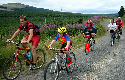
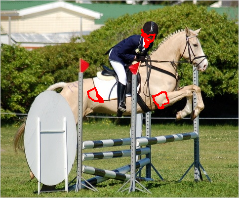
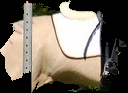
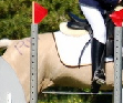
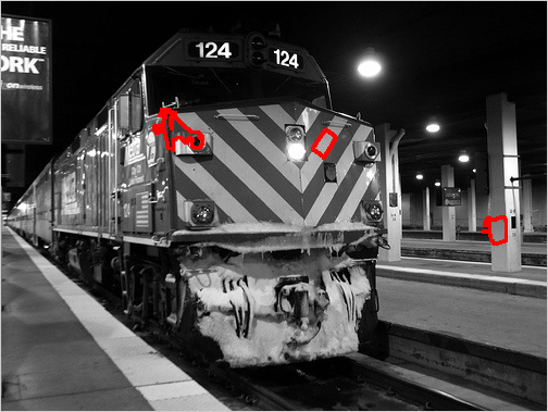
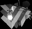
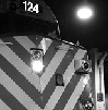
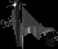
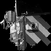
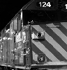
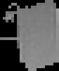
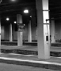
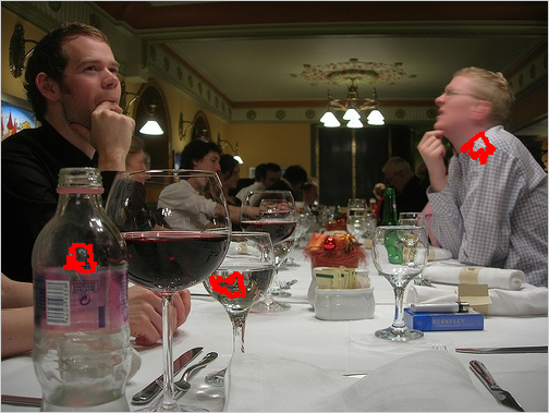
Figure 3: Showing three superpixels in each image (top), followed by corresponding zoom-out regions that are seen by the segmenation process, (left) superpixel, (center) proximal region, (right) distant. As we zoom in from image to the superpixel level, it becomes increasingly hard to tell what we are looking at, however the higher zoom-out levels provide rich contextual information.

2.1.3 Distant zoom

Zooming out further, we move to the distant level: a region large enough to include sizeable fractions of objects, and sometimes entire objects. At this level our scope is wide enough to allow reasoning about shape, presence of more complex patterns in color and gradient, and the spatial layout of such patterns. Therefore we can expect more complex features that represent these properties to be useful here. Distant regions are more likely to straddle true boundaries in the image, and so this higher-level feature extraction may include a significant area in both the category of the superpixel at hand and nearby categories. For example, consider a person sitting on a chair; bottle on a dining table; pasture animals on the background of grass, etc. Naturally we expect this to provide useful information on both the appearance of a class and its context.

For neighboring superpixels, distant regions will have a very large overlap; superpixels which are one superpixel apart will have significant, but lesser, overlap in their distant regions; etc., all the way to superpixels that are sufficiently far apart that the distant regions do not overlap and thus are independent given the scene. This overlap in the regions is likely to lead to somewhat gradual changes in features, and to impose an entire network of implicit smoothness “terms”, which depend both on the distance in the image and on the similarity in appearance in and around superpixels. Imposing such smoothness in a CRF usually leads to a very complex, intractable model.

2.1.4 Global zoom

The final zoom-out scope is the entire scene. Features computed at this level capture “what kind of an image” we are looking at. One aspect of this global context is image-level classification: since state of the art in image classification seems to be dramatically higher than that of detection or segmentation [9, 30] we can expect image-level features to help determine presence of categories in the scene and thus guide the segmentation.

More subtly, features that are useful for classification can be directly useful for global support of local labeling decisions; e.g., lots of green in an image supports labeling a (non-green) superpixel as cow or sheep more than it supports labeling that superpixel as chair or bottle, other things being equal. On the other hand, lots of straight vertical lines in an image would perhaps suggest man-made environment, thus supporting categories relevant to indoors or urban scenes more than, say, wildlife.

At this global level, all superpixels in an image will of course have the same features, imposing (implicit, soft) global constraints. This is yet another form of high-order interaction that is hard to capture in a CRF framework, despite numerous attempts [3].

2.2 Learning to label with asymmetric loss

Once we have computed the zoom-out features we simply concatenate them into a feature vector representing a superpixel. For superpixel $s$ in image $\mathcal{I}$, we will denote this feature vector as

$$\bm{\phi}_{\text{zoom-out}}(s,\mathcal{I})\,=\,\begin{bmatrix}\bm{{\color[rgb]{1,0,0}\phi}}_{{\color[rgb]{1,0,0}loc}}(s,\mathcal{I})\\ \bm{{\color[rgb]{0,1,1}\phi}}_{{\color[rgb]{0,1,1}prox}}(s,\mathcal{I})\\ \bm{{\color[rgb]{1,.5,0}\phi}}_{{\color[rgb]{1,.5,0}dist}}(s,\mathcal{I})\\ \bm{{\color[rgb]{0.472,0.472,0.472}\phi}}_{{\color[rgb]{0.472,0.472,0.472}glob}}(\mathcal{I})\end{bmatrix}$$ (1)

For the training data, we will associate a single category label $y_{s}$ with each superpixel $s$. This decision carries some risk, since in any non-trivial over-segmentation some of the superpixels will not be perfectly aligned with ground truth boundaries. In section 4 we evaluate this risk empirically for our choice of superpixel settings and confirm that it is indeed minimal.

Now we are ready to train a classifier that maps $s$ in image $\mathcal{I}$ to $y_{s}$ based on $\bm{\phi}_{\text{zoom-out}}$; this requires choosing the empirical loss function to be minimized, subject to regularization. In semantic segmentation settings, a factor that must impact this choice is the highly imbalanced nature of the labels. Some categories are much more common than others, but our goal (encouraged by the way benchmark like VOC evaluate segmentations) is to predict them equally well. It is well known that training on imbalanced data without taking precautions can lead to poor results [10, 29, 22]. A common way to deal with this is to stratify the training data; in practice this means that we throw away a large fraction of the data corresponding to the more common classes. We follow an alternative which we find less wasteful, and which in our experience often produces dramatically better results: use all the data, but change the loss. There has been some work on loss design for learning segmentation [35], but the simple weighted loss we describe below has to our knowledge been missed in segmentation literature, with the exception of [20] and [22], where it was used for binary segmentation.

Let the frequency of class $c$ in the training data be $f_{c}$, with $\sum_{c}f_{c}=1$. Suppose our choice of loss is log-loss; we modify it to be

$$-\frac{1}{N}\sum_{i=1}^{N}\frac{1}{f_{y_{i}}}\log\widehat{p}\left(y_{i}|\bm{\phi}(s_{i},\mathcal{I}_{i})\right),$$ (2)

where $\widehat{p}\left(y_{i}|\bm{\phi}(s_{i},\mathcal{I}_{i})\right)$ is the estimated probability of the correct label for segment $s_{i}$ in image $\mathcal{I}_{i}$, according to our model. In other words, we scale the loss by the inverse frequency of each class, effectively giving each pixel of less frequent classes more importance. This modification does not change loss convexity, and only requires minor changes in the optimization code, e.g., back-propagation.

3 Related work

The literature on segmentation is vast, and here we only mention work that is either significant as having achieved state of the art performance in recent times, or is closely related to ours in some way. In Section 4 we compare our performance to that of most of the methods mentioned here.

Many prominent segmentation methods rely on conditional random fields (CRF) over nodes corresponding to pixels or superpixels. Such models incorporate local evidence in unary potentials, while interactions between label assignments are captured by pairwise and possibly higher-order potentials. This includes various hierarchical CRFs [31, 21, 22, 3]. In contrast, we let the zoom-out features (in CRF terminology, the unary potentials) to capture higher-order structure.

Another recent trend has been to follow a multi-stage approach: First a set of proposal regions is generated, by a category-independent [6, 36] or category-aware [2] mechanism. Then the regions are scored or ranked based on their compatibility with the target classes. Work in this vein includes [4, 17, 2, 5, 24]. A similar approach is taken in [37], where multiple segmentations obtained from [4] are re-ranked using a discriminatively trained model. Recent advances along these lines include [15], which uses convnets and [8], which improves upon the re-ranking in [37], also using convnet-based features. At submission time, these two lines of work are roughly tied for the previous state of the art, with mean accuracy of 51.6% and 52.2%, respectively, on VOC 2012 test. In contrast to most of the work in this group, we do not rely on region generators, and limit preprocessing to over-segmentation of the image into a large number of superpixels.

A body of work examined the role of context and the importance of non-local evidence in segmentation. The idea of computing features over a neighborhood of superpixels for segmentation purposes was introduced in [11] and [25]; other early work on using forms of context for segmentation includes [31]. A study in [27] concluded that non-unary terms may be unnecessary when neighborhood and global information is captured by unary terms, but the results were significantly inferior to state of the art at the time.

Recent work closest to ours includes [10, 29, 33, 28, 16]. In [10], the same convnet is applied on different resolutions of the image and combined with a tree-structured graph over superpixels to impose smoothness. In [28] the features applied to multiple levels (roughly analogous to our local+proximal+global) are also same, and hand-crafted instead of using convnets. In [29] there is also a single convnet, but it is applied in a recurrent fashion, i.e., input to the network includes, in addition to the scaled image, the feature maps computed by the network at a previous level. A similar idea is pursued in [16], where it is applied to boundary detection in 3D biological data. In contrast with all of these, we use different feature extractors across levels, some of them with a much smaller receptive field than any of the networks in the literature. We show in Section 4 that our approach obtains better performance (on Stanford Background Dataset) than that reported for [10, 29, 33, 28]; no comparison to [16] is available.

Finally, two pieces of concurrent work share some key ideas with our work, and we discuss these in some detail here. In [26], achieving 62.2% mean accuracy on VOC 2012 test, a 16-layer convnet is applied to an image at a coarse grid of locations. Predictions based on the final layer of the network are upsampled and summed with predictions made from intermediate layers of the network. Since units in lower layers are associated with smaller receptive field than those in the final layer, this mechanism provides fusion of information across spatial levels, much like our zoom-out features. The architecture in [26] is more efficient than our current implementation since it reuses computation efficiently (via framing the computation of features at multiple locations as convolution), and since the entire model is trained end-to-end. However, it relies in a somewhat reduced range of spatial context compared to our work; using our terminology proposed above, the architecture in [26] roughly analogous to combining our proximal and distant zoom-out levels, along with another one above distant, but without the global level, important to establish the general scene context, and without the local level, important for precise localization of boundaries. Also, we choose to “fuse” not the predictions made at different levels, but the rich evidence (features themselves).

The other recent work with significant similarities to ours is [13], where hypercolumns are formed by pooling evidence extracted from nested regions around a pixel; these too resemble our zoom-out feature representations. In contrast with [26] and with our work, the input to the system here consists of a hypothesized detection bounding box, and not an entire image. The hypercolumn includes some local information (obtained from the pool2 layer) as well as information pooled from regions akin to our proximal as well as the level that is global relative to the hypothesized bounding box, but is not global with respect to the entire image. A further difference from our work is the use of location-specific classifiers within the bounding box, instead of the same classifer applied everywhere. This work achieves 59.0% mean accuracy on VOC 2012 test.

4 Experiments

Our main set of experiments focuses on the PASCAL VOC category-level segmentation benchmark with 21 categories, including the catch-all background category. VOC is widely considered to be the main semantic segmentation benchmark today. The original data set labeled with segmentation ground truth consists of train and val portions (about 1,500 images in each). Ground truth labels for additional 9,118 images have been provided by authors of [14], and are commonly used in training segmentation models. In all experiments below, we used the combination of these additional images with the original train set for training, and val was used only as held out validation set, to tune parameters and to perform “ablation studies”.

The main measure of success is accuracy on the test, which for VOC 2012 consists of 1,456 images. No ground truth is available for test, and accuracy on it can only be obtained by uploading predicted segmentations to the evaluation server. The standard evaluation measure for category-level segmentation in VOC benchmarks is per-pixel accuracy, defined as intersection of the predicted and true sets of pixels for a given class, divided by their union (IU in short). This is averaged across the 21 classes to provide a single accuracy number, mean IU, usually used to measure overall performance of a method.

4.1 Superpixels and neighborhoods

We obtained roughly 500 SLIC superpixels [1] per image (the exact number varies per image), with the parameter $m$ that controls the tradeoff between spatial and color proximity set to 15, producing superpixels which tend to be of uniform size and regular shape, but adhere to local boundaries when color evidence compels it. This results in average supepixel region of 21$\times$21 pixels. An example of a typical over-segmentation is shown in Figure 2.

Proximal region for a superpixel $s$ is defined as a set of superpixels within radius 2 from $s$, that is, the immediate neighbors of $s$ as well as their immediate neighbors. The proximal region can be of arbitrary shape; its average size in training images is 100x100 pixels. The distant region is defined by all neighbors of $s$ up to the 3rd degree, and consists of the bounding box around those neighbors, so that in contrast to proximal, it is always rectangular; its average size is 170$\times$170 pixels. Figure 2 contains a few typical examples for the regions.

4.2 Zoom-out feature computation

Feature extraction differs according to the zoom-out level, as described below.

4.2.1 Local features

To represent a superpixel we use a number of well known features as well as a small set of learned features.

Color

We compute histograms separately for each of the three L*a*b color channels, using 32 as well as 8 bins, using equally spaced binning; this yields 120 feature dimensions. We also compute the entropy of each 32-bin histogram as an additional scalar feature (+3 dimensions). Finally, we also re-compute histograms using adaptive binning, based on observed quantiles in each image (+120 dimensions).

Texture

Texture is represented by histogram of texton assignments, with 64-texton dictionary computed over a sampling of images from the training set. This histogram is augmented with the value of its entropy. In total there are 65 texture-related channels.

SIFT

A richer set of features capturing appearance is based on “bag of words” representations computed over SIFT descriptors. The descriptors are computed over a regular grid (every 8 pixels), on 8- and 18-pixel patches, separately for each L*a*b channel. All the descriptors are assigned to a dictionary of 500 visual words. Resulting assignment histograms are averaged for two patch sizes in each channel, yielding a total of 1500 values, plus 6 values for the entropies of the histograms.

Location

Finally, we encode superpixel’s location, by computing its image-normalized coordinates relative to the center as well as its shift from the center (the absolute value of the coordinates); this produces four feature values.

Local convnet

Instead of using hand-crafted features we could learn a representation for the superpixel using a convnet. We trained a network with 3 convolutional (conv) + pooling + RELU layers, with 32, 32 and 64 filters respectively, followed by two fully connected layers (1152 units each) and finally a softmax layer. The input to this network is the bounding box of the superpixel, resized to 25$\times$25 pixels and padded to $35\times 35$, in L*a*b color space. The filter sizes in all layers are 5$\times$5; the pooling layers all have 3$\times$3 receptive fields, with stride of 2. We trained the network using back-propagation, with the objective of minimizing log-loss for superpixel classification. The output of the softmax layer of this network is used as a 21-dimensional feature vector. Another network with the same architecture was trained on binary classification of foreground vs. background classes; that gives us two more features.

4.2.2 Proximal features

We use the same set of handcrafted features as for local regions, resulting in 1818 feature dimensions.

4.2.3 Distant and global features

For distant and global features we use deep convnets originally trained to classify images. In our initial experiments we used the CNN-S network in [7]. It has 5 convolution layers (three of them followed by pooling) and two fully connected layers. To extract the relevant features, we resize either the distant region or the entire image to 224$\times$224 pixels, feed it to the network, and record the activation values of the last fully-connected layer with 4096 units. In a subsequent set of experiments we switched from CNN-S to a 16 layer network introduced in [32]. This network, which we refer to as VGG-16, contains more layers that apply non-linear transformations, but with smaller filters, and thus may learn richer representation with fewer parameters. It has produced excellent results on image classification and recently has been reported to lead to a much better performance when used in detection [12]. As reported below, we also observe a significant improvement when using VGG-16 to extract distant and global features, compared to performance with CNN-S. Note that both networks we used were originally trained for 1000-category ImageNet classification task, and we did not fine-tune it in any way on VOC data.

4.3 Learning setup

With more than 10,000 images and roughly 500 superpixels per image, we have more than 5 million training examples.

In section 2 we mentioned an obvious concern when reducing image labeling problem to superpixel labeling is whether this leads to loss of achievable accuracy, since superpixels need not perfectly adhere to true boundaries. Having assigned each superpixel a category label based on the majority of pixels in it, we computed the accuracy of this assignment on val: 94.4%. Since accuracies of most of today’s methods are well below this number, we can assume that any potential loss of accuracy due to our commitment to superpixel boundaries is going to play a minimal role in our results.

We trained the classifiers mentioned below with asymmetric loss (2) using Caffe [18], on a single machine equipped with a Tesla K40 GPU. During training we used fixed learning rate of 0.0001, and weight decay factor of 0.001.

4.4 Results on PASCAL VOC 2012

To empirically assess the importance of features extracted at different zoom-out levels, we trained linear (softmax) models using various feature subsets, as shown in Table 1, and evaluated them on VOC 2012 val. In these experiments we used CNN-S to extract distant and global features.

Figure 4: Color code for VOC categories. Background is black.

Feature set	mean accuracy
local	14.6
proximal	15.5
local+proximal	17.7
local+distant	37.38
local+global	41.8
local+proximal+global	43.4
distant+global	47.0
full zoom-out, symmetric loss	20.4
full zoom-out, asymmetric loss	52.4

Table 1: Ablation study: importance of features from different levels under linear superpixel classification. Results on VOC 2012 val, mean class accuracy.

It is evident that each of the zoom-out levels contributes to the eventual accuracy. The most striking is the effect of adding the distant and global features computed by convnets; but local and proximal features are very important as well, and without those we observe poor segment localization. We also confirmed empirically that learning with asymmetric loss leads to dramatically better performance, as shown in Table 1, with a few examples in Figure 5.

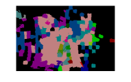
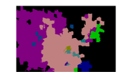
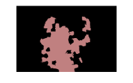
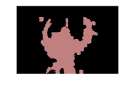
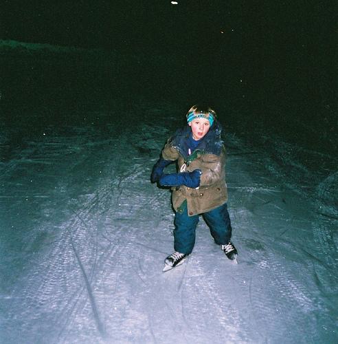
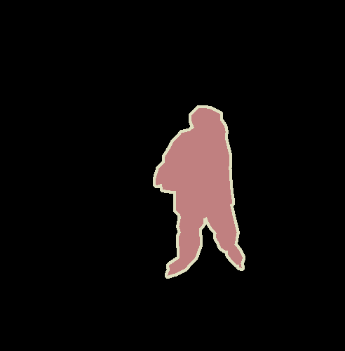
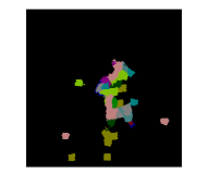
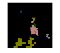
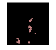
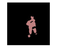
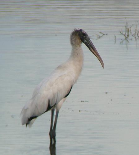
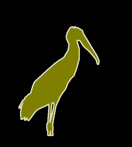
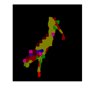
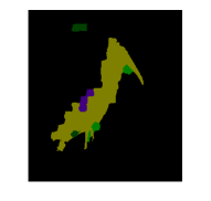
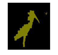
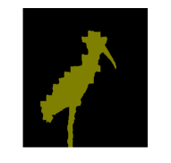
Figure 5: Examples illustrating the effect of zoom-out levels. From left: original image, ground truth, local only, local and proximal, local, proximal and global, and the full (four levels) set of zoom-out features. In all cases a linear model is used to label superpixels. See Figure 4 for category color code.

Next we explored the impact of switching from linear softmax models to multilayer neural networks, as well as the effect of switching from the 7-layer CNN-S to VGG-16. Results of this set of experiments (mean IU when testing on val) are shown in Table 2. The best performer in the set of experiments using CNN-S was a two-layer network with 512 hidden units with rectified linear unit activations. Deeper networks tended to generalize less well, even when using dropout [19] in training. Then, switching to VGG-16, we explored classifiers with this architecture, varying the number of hidden units. The model with 1024 units in the hidden layer led to the best accuracy on val.

net	#layers	#units	mean IoU
CNN-S	1 (linear)	0	52.4
CNN-S	2	256	57.9
CNN-S	2	512	59.1
CNN-S	3	256+256	56.4
CNN-S	3	256+256(dropout)	57.0
VGG-16	2	256	62.3
VGG-16	2	512	63.0
VGG-16	2	1024	63.5

Table 2: Results on VOC 2012 val with different classification models. Net: convnet used to extract proximal and global features: CNN-S is the 7-layer network from [7], VGG-16 is the 16-layer network from [32]. Both convnets were pre-trained on ImageNet and used with no fine-tuning for our task. #layers: number of layers in the classifier network. #units: number of units in the hidden layer of the classifier network.

Based on the results in Table 2 we took the 2-layer network with 1024 hidden units, with distant and global features extracted using VGG-16, as the model of choice, and evaluated it on the VOC 2012 test data. We report the results of this evaluation in Table 3; to allow for comparison to previously published results, we also include numbers on VOC 2010 and 2011 test sets, which are subsets of 2012. The table makes it clear that our zoom-out architecture achieves accuracies well above those of any of the previously published methods. Detailed per-class accuracies in Table 4 reveal that this superiority is obtained on 15 out of 20 object categories, some of them (like dogs, cats, or trains) by a large margin.

Method	VOC2010	VOC2011	VOC2012
zoom-out (ours)	64.4	64.1	64.4
FCN-8s [26]	–	62.7	62.2
Hypercolumns [13]	–	–	59.2
DivMbest+convnet [8]	–	–	52.2
SDS [15]	–	52.6	51.6
DivMbest+rerank [37]	–	–	48.1
Codemaps [24]	–	–	48.3
$O2P$ [4]	–	47.6	47.8
Regions & parts[2]	–	40.8	–
D-sampling [27]	33.5	–	–
Harmony potentials [3]	40.1	–	–

Table 3: Results on VOC 2010, 2011 and 2012 test. Mean IoU is shown, see Table 4 for per-class accuracies of the zoom-out method.

class	mean	background	aeroplane	bycycle	bird	boat	bottle	bus	car	cat	chair	cow	diningtable	dog	horse	motorbike	person	potted plant	sheep	sofa	train	TV/monitor
acc	64.4	89.8	81.9	35.1	78.2	57.4	56.5	80.5	74.0	79.8	22.4	69.6	53.7	74.0	76.0	76.6	68.8	44.3	70.2	40.2	68.9	55.3

Table 4: Detailed results of our method on VOC 2012 test. Bold indicates best results on a given class of any method we are aware of.

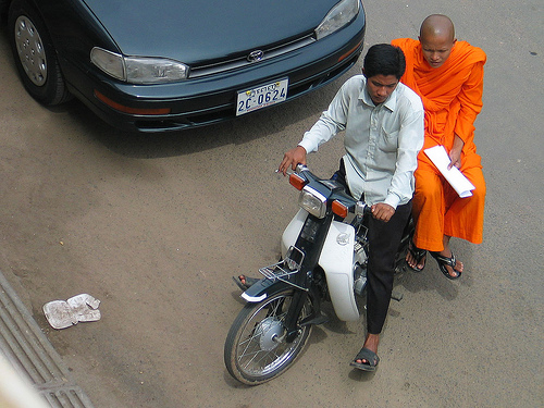
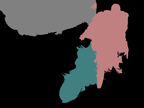
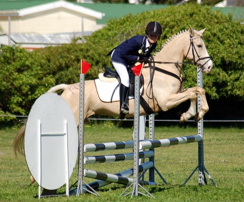
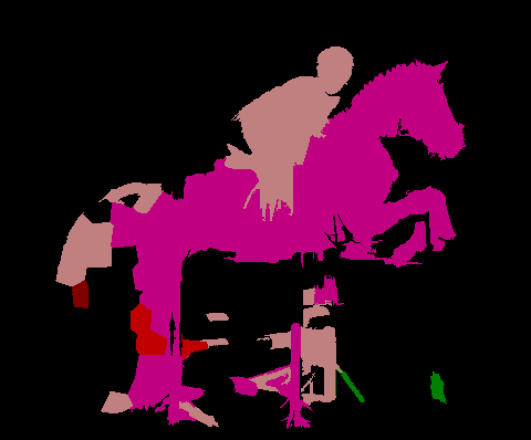
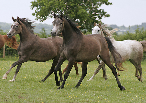
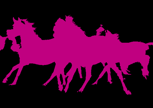
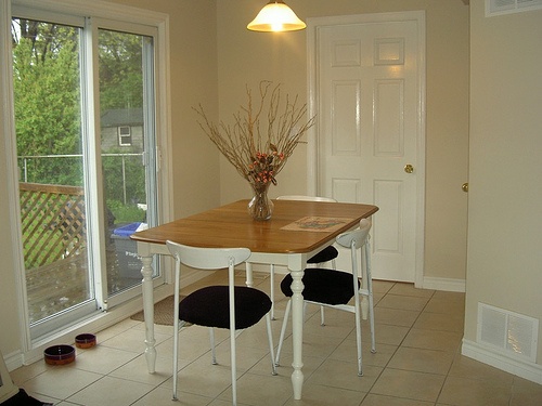
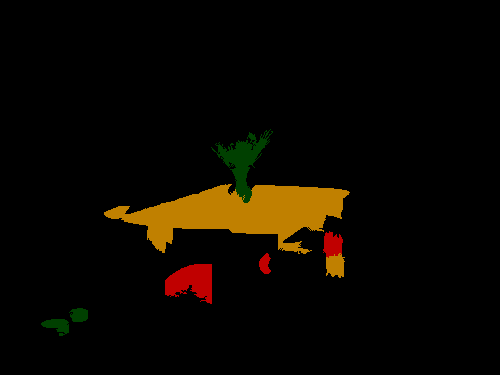
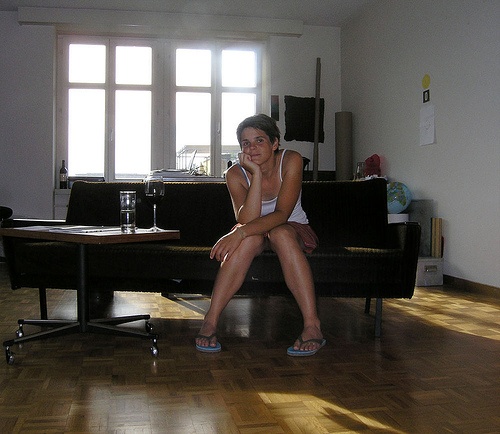
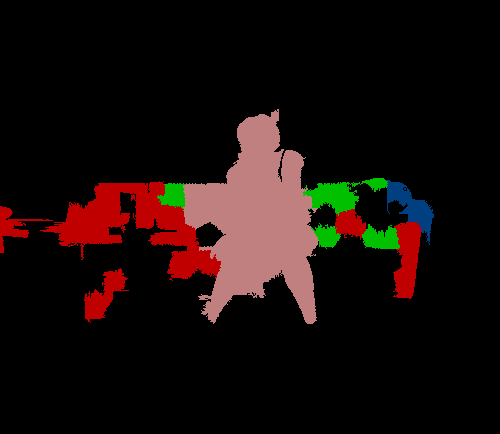
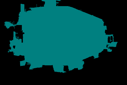
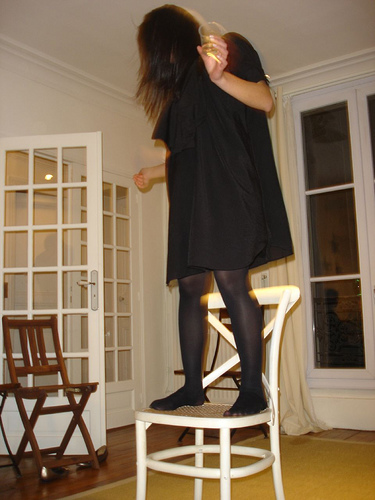
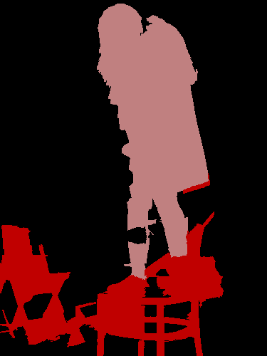
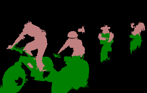
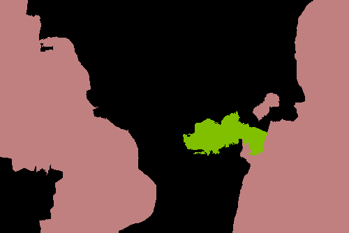
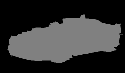
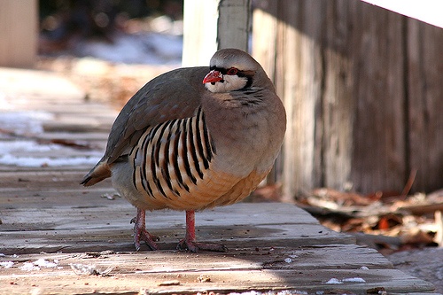
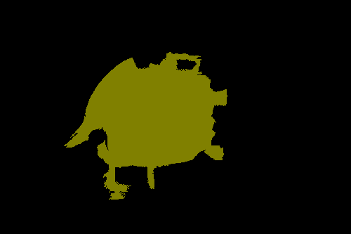
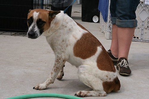
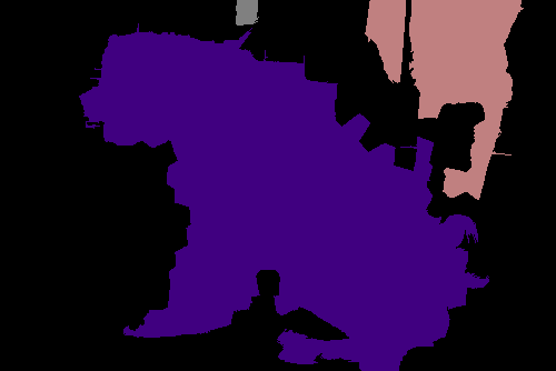
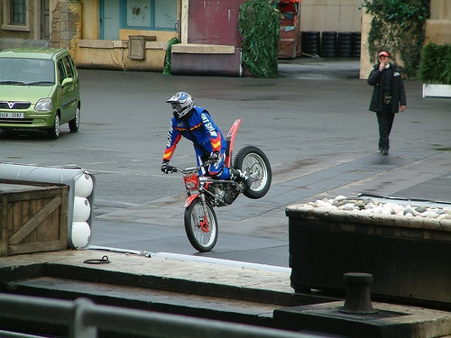
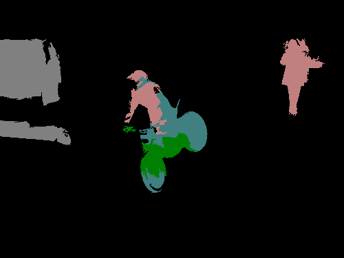
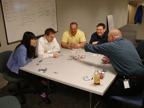
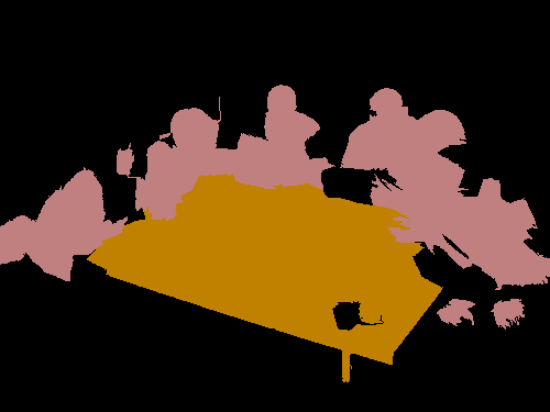
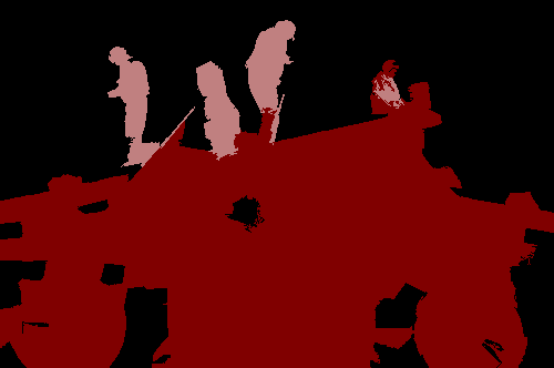
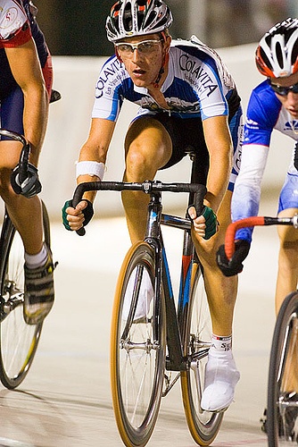
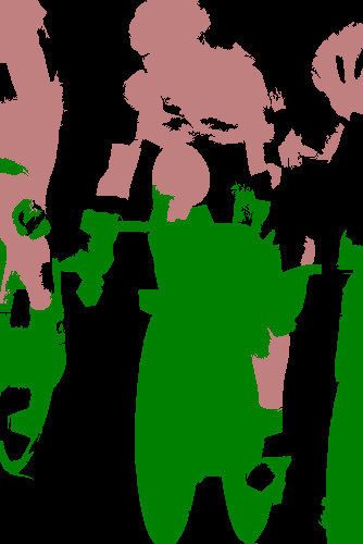
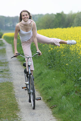
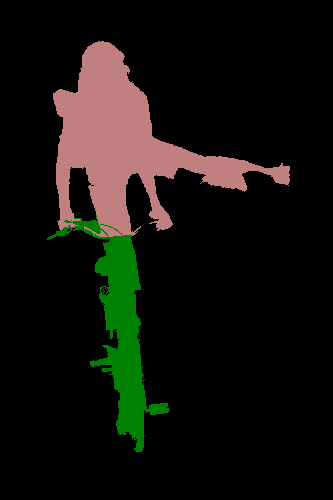
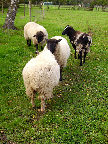
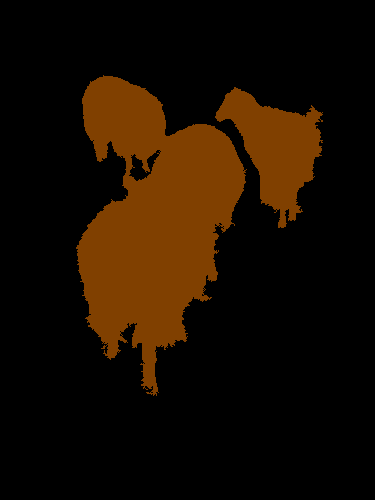
Figure 6: Example segmentations on VOC 2012 val with our best classifier (2-layer neural network with 1024 hidden units, using four zoom-out levels). See Figure 4 for category color code.

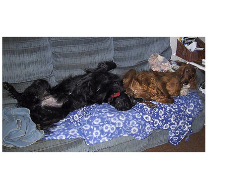
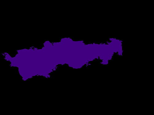
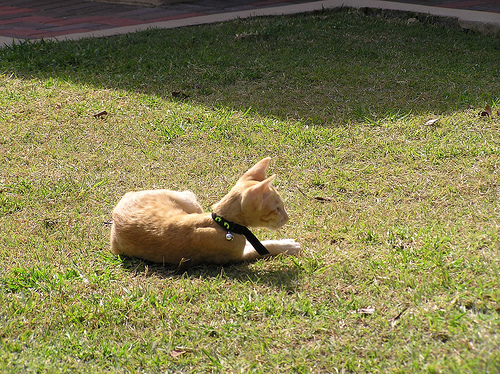
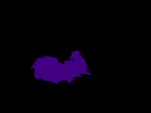
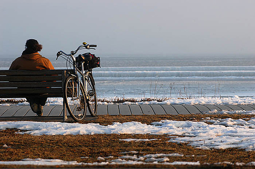
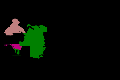
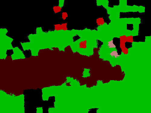
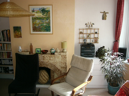
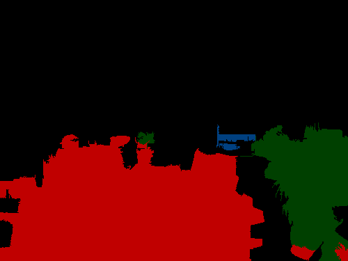
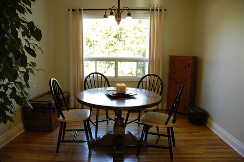
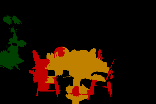
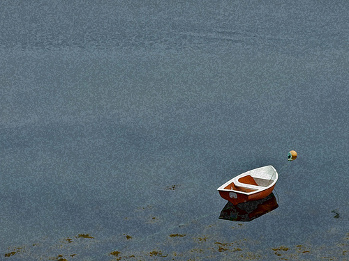
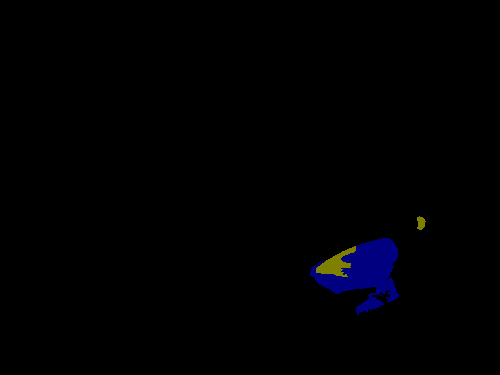
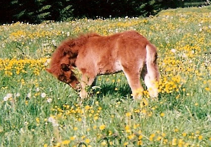
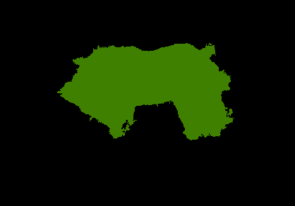
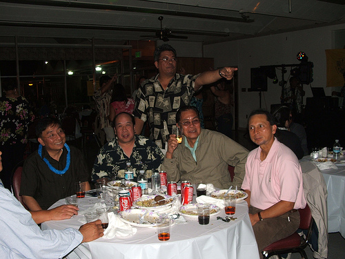
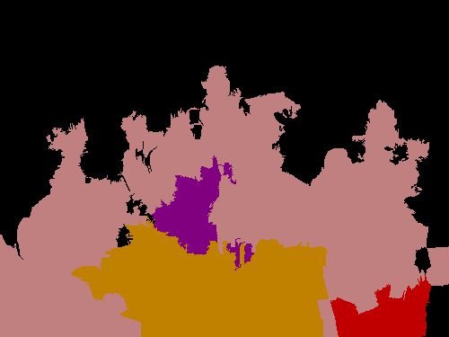
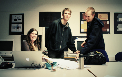
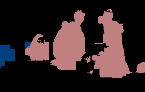
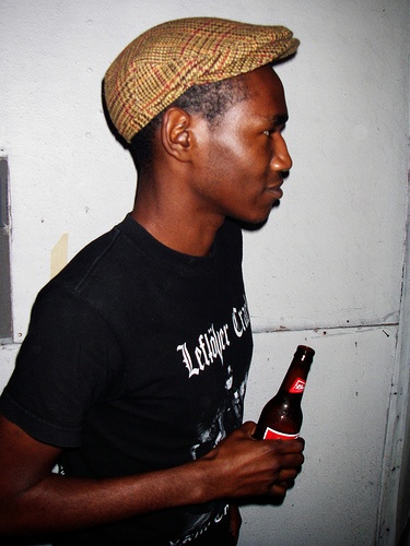
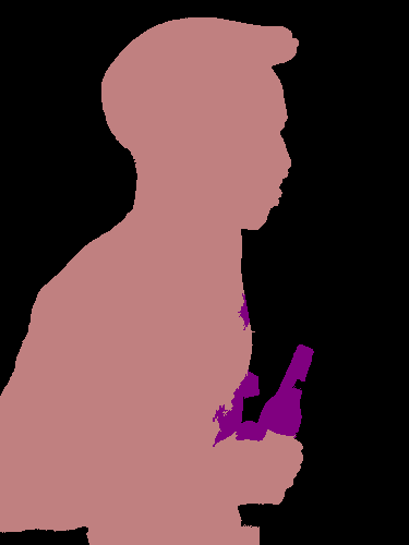
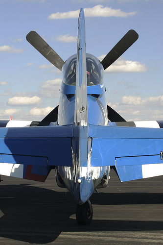
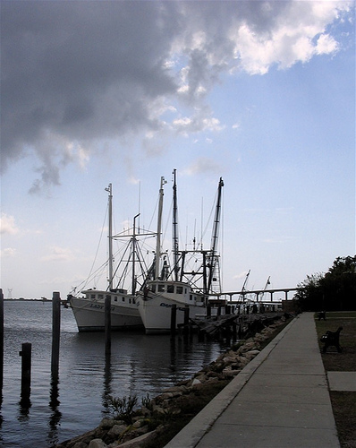
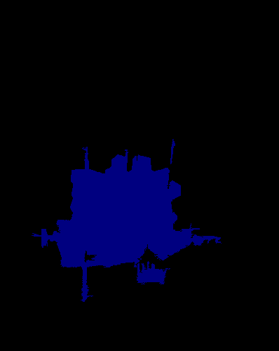
Figure 7: Additional examples of segmentation on VOC 2012 val with our model. See Figure 4 for category color code.

Figure 6 displays example segmentations. Many of the segmentations have moderate to high accuracy, capturing correct classes, in correct layout, and sometimes including level of detail that is usually missing from over-smoothed segmentations obtained by CRFs or generated by region proposals. But there is tradeoff: despite the smoothness imposed by higher zoom-out levels, the segmentations we get do tend to be under-smoothed, and in particular include little “islands” of often irrelevant categories. To some extent this might be alleviated by post-processing; we found that we could learn a classifier for isolated regions that with reasonable accuracy decides when these must be “flipped” to the surrounding label, and this improves results on val by about 0.5%, while making the segmentations more visually pleasing. We do not pursue this ad-hoc approach, and instead discuss in Section 5 more principled remedies that should be investigated in the future.

4.5 Results on Stanford Background Dataset

For some of the closely related recent work results on VOC are not available, so to allow for empirical comparison, we also ran an experiment on Stanford Background Dataset (SBD). It has 715 images of outdoor scenes, with dense labels for eight categories. We applied the same zoom-out architecture to this dataset as to VOC, with two exceptions: (i) the local convnet produced 8 features instead of 21+2, and (ii) the classifier was smaller, with only 128 hidden units, since SBD has about 20 times fewer examples than VOC and thus could not support training larger models.

There is no standard train/test partition of SBD; the established protocol calls for reporting 5-fold cross validation results. There is also no single performance measure; two commonly reported measures are per-pixel accuracy and average class accuracy (the latter is different from the VOC measure in that it does not directly penalize false positives).

Method	pixel accuracy	class accuracy
zoom-out (ours)	82.1	77.3
Multiscale convnet [10]	81.4	76.0
Recurrent CNN [29]	80.2	69.9
Pylon [22]	81.9	72.4
Recursive NN [33]	78.1	–
Multilevel [28]	78.4	–

Table 5: Results on Stanford Background Dataset

The resuls in Table 5 show that the zoom-out architecture obtains results better than those in [29] and [10], both in class accuracy and in pixel accuracy.

5 Conclusions

The main point of this paper is to explore how far we can push feedforward semantic labeling of superpixels when we use multilevel, zoom-out feature construction and train non-linear classifiers (multi-layer neural networks) with asymmetric loss. The results are perhaps surprising: we can far surpass existing state of the art, despite apparent simplicity of our method and lack of explicit respresentation of the structured nature of the segmentation task. Another important conclusion that emerges from this is that we finally have shown that segmentation, just like image classification, detection and other recognition tasks, can benefit from the advent of deep convolutional networks.

Despite this progress, much remains to be done as we continue this work. Immediately, we plan to explore obvious improvements. One of these is replacement of all the handcrafted local and proximal features with features learned from the data with convnets. Another such improvement is to fine tune the “off the shelf” networks currently used for distant and global feature extraction. We also plan to look into including additional zoom-out levels. Our longer term plan is to switch from a collection of feature extractors deployed at different zoom-out levels to a single zoom-out network, which would be more in line with the philosophy of end-to-end learning that has drive deep learning research.

Finally, despite the surprising success of the zoom-out architecture described here, we by no means intend to entirely dismiss CRFs, or more generally inference in structured models. We believe that the zoom-out architecture may eventually benefit from bringing back some form of inference to “clean up” the predictions. We hope that this can be done without giving up the feedforward nature of our approach; one possibility we are interested in exploring is to “unroll” approximate inference into additional layers in the feedforward network [23, 34].

References

- [1] R. Achanta, A. Shaji, K. Smith, A. Lucchi, P. Fua, and S. S sstrunk. Slic superpixels compared to state-of-the-art superpixel methods. IEEE TPAMI, 2012.
- [2] P. Arbelaez, B. Hariharan, C. Gu, S. Gupta, L. Bourdev, and J. Malik. Semantic segmentation using regions and parts. In CVPR, 2012.
- [3] X. Boix, J. M. Gonfaus, J. van de Weijer, A. D. Bagdanov, J. S. Gual, and J. Gonzàlez. Harmony potentials - fusing global and local scale for semantic image segmentation. IJCV, 96(1):83–102, 2012.
- [4] J. Carreira, R. Caseiro, J. Batista, and C. Sminchisescu. Semantic segmentation with second-order pooling. In Computer Vision–ECCV 2012, pages 430–443. Springer, 2012.
- [5] J. Carreira, F. Li, and C. Sminchisescu. Object recognition by sequential figure-ground ranking. IJCV, 98(3):243–262, 2012.
- [6] J. Carreira and C. Sminchisescu. Cpmc: Automatic object segmentation using constrained parametric min-cuts. Pattern Analysis and Machine Intelligence, IEEE Transactions on, 34(7), 2012.
- [7] K. Chatfield, K. Simonyan, A. Vedaldi, and A. Zisserman. Return of the devil in the details: Delving deep into convolutional nets. In BMVC, 2014.
- [8] M. Cogswell, X. Lin, and D. Batra. Personal communication. November 2014.
- [9] M. Everingham, S. Eslami, L. Van Gool, C. Williams, J. Winn, and A. Zisserman. The pascal visual object classes challenge: A retrospective. International Journal of Computer Vision, 2014.
- [10] C. Farabet, C. Couprie, L. Najman, and Y. LeCun. Learning hierarchical features for scene labeling. IEEE TPAMI, 35(8), 2013.
- [11] B. Fulkerson, A. Vedaldi, and S. Soatto. Class segmentation and object localization with superpixel neighborhoods. In CVPR, 2009.
- [12] R. Girshick, J. Donohue, T. Darrell, and J. Malik. Rich feature hierarchies for accurate object detection and semantic segmentation. arXiv preprint http://arxiv.org/abs/1311.2524, 2014.
- [13] B. Hariharan, P. A. an R. Girshick, and J. Malik. Hypercolumns for object segmentation and fine-grained localization. arXiv preprint http://arxiv.org/abs/1411.5752, 2014.
- [14] B. Hariharan, P. Arbelaez, L. Bourdev, S. Maji, and J. Malik. Semantic contours from inverse detectors. In International Conference on Computer Vision (ICCV), 2011.
- [15] B. Hariharan, P. Arbeláez, R. Girshick, and J. Malik. Simultaneous detection and segmentation. In Computer Vision–ECCV 2014, 2014.
- [16] G. B. Huang and V. Jain. Deep and wide multiscale recursive networks for robust image labeling. arXiv preprint arXiv:1310.0354, 2013.
- [17] A. Ion, J. Carreira, and C. Sminchisescu. Probabilistic joint image segmentation and labeling. In NIPS, pages 1827–1835, 2011.
- [18] Y. Jia, E. Shelhamer, J. Donahue, S. Karayev, J. Long, R. Girshick, S. Guadarrama, and T. Darrell. Caffe: Convolutional architecture for fast feature embedding. arXiv preprint arXiv:1408.5093, 2014.
- [19] A. Krizhevsky, I. Sutskever, and G. E. Hinton. Imagenet classification with deep convolutional neural networks. In NIPS, 2012.
- [20] D. Kuettel, M. Guillaumin, and V. Ferrari. Segmentation propagation in imagenet. In ECCV, 2012.
- [21] L. Ladickỳ, C. Russell, P. Kohli, and P. H. S. Torr. Associative hierarchical CRFs for object class image segmentation. ICCV, 2009.
- [22] V. Lempitsky, A. Vedaldi, and A. Zisserman. Pylon model for semantic segmentation. In NIPS, pages 1485–1493, 2011.
- [23] Y. Li and R. Zemel. Mean field networks. In ICML Workshop on Learning Tractable Probabilistic Models, 2014.
- [24] Z. Li, E. Gavves, K. E. A. van de Sande, C. G. M. Snoek, and A. W. M. Smeulders. Codemaps segment, classify and search objects locally. In ICCV, 2013.
- [25] J. J. Lim, P. Arbeláez, C. Gu, and J. Malik. Context by region ancestry. In ICCV, 2009.
- [26] J. Long, E. Shelhamer, and T. Darrell. Fully convolutional networks for semantic segmentation. arXiv preprint http://arxiv.org/abs/1411.4038, 2014.
- [27] A. Lucchi, Y. Li, X. Boix, K. Smith, and P. Fua. Are spatial and global constraints really necessary for segmentation? In ICCV, 2011.
- [28] M. Mostajabi and I. Gholampour. A robust multilevel segment description for multi-class object recognition. Machine Vision and Applications, 2014.
- [29] P. H. O. Pinheiro and R. Collobert. Recurrent convolutional neural networks for scene labeling. In ICML, 2014.
- [30] O. Russakovsky, J. Deng, H. Su, J. Krause, S. Satheesh, S. Ma, Z. Huang, A. Karpathy, A. Khosla, M. Bernstein, et al. Imagenet large scale visual recognition challenge. arXiv:1409.0575, 2014.
- [31] J. Shotton, J. Winn, C. Rother, and A. Criminisi. Textonboost for image understanding: Multi-class object recognition and segmentation by jointly modeling texture, layout, and context. IJCV, 81(1), 2009.
- [32] K. Simonyan and A. Zisserman. Very deep convolutional networks for large-scale image recognition. arXiv preprint http://arxiv.org/abs/1409.1556, 2014.
- [33] R. Socher, C. C. Lin, A. Y. Ng, and C. D. Manning. Parsing Natural Scenes and Natural Language with Recursive Neural Networks. In ICML, 2011.
- [34] V. Stoyanov, A. Ropson, and J. Eisner. Empirical risk minimization of graphical model parameters given approximate inference, decoding, and model structure. In AISTATS, 2011.
- [35] D. Tarlow and R. S. Zemel. Structured output learning with high order loss functions. In AISTATS, 2012.
- [36] J. R. R. Uijlings, K. E. A. van de Sande, T. Gevers, and A. W. M. Smeulders. Selective search for object recognition. International Journal of Computer Vision, 104(2), 2013.
- [37] P. Yadollahpour, D. Batra, and G. Shakhnarovich. Discriminative re-ranking of diverse segmentations. In CVPR, 2013.