A Generalization of the Chambolle-Pock Algorithm to Banach Spaces with Applications to Inverse Problems

Abstract

For a Hilbert space setting Chambolle and Pock introduced an attractive first-order algorithm which solves a convex optimization problem and its Fenchel dual simultaneously. We present a generalization of this algorithm to Banach spaces. Moreover, under certain conditions we prove strong convergence as well as convergence rates. Due to the generalization the method becomes efficiently applicable for a wider class of problems. This fact makes it particularly interesting for solving ill-posed inverse problems on Banach spaces by Tikhonov regularization or the iteratively regularized Newton-type method, respectively.

1 Introduction

Let $X$ and $Y$ be real Banach spaces and $T:X\to Y$ a linear, continuous operator, with adjoint $T^{*}:Y^{*}\to X^{*}$. In this paper we will consider the convex optimization problem

$$\bar{x}=\text{argmin}_{x\in X}\left(g(Tx)+f(x)\right)\qquad\mathbf{(P)}$$ (1)

as well as its Fenchel dual problem

$$\bar{p}=\operatorname*{argmax}\limits_{p\in Y^{*}}\left(-f^{*}(T^{*}p)-g^{*}(-p)\right),\qquad\mathbf{(D)}$$ (2)

where $f:X\to[0,+\infty)$ and $g:Y\to[0,+\infty)$ belong to the class $\Gamma(X)$ and $\Gamma(Y)$ of proper, convex and lower semicontinuous (l.s.c.) functions. By $f^{*}\in\Gamma(X^{*})$ and $g^{*}\in\Gamma(Y^{*})$ we denote their conjugate functions. A problem of the form $\mathbf{(P)}$ arises in many applications, such as image deblurring (e.g. the ROF model [24]), sparse signal restoration (e.g. the LASSO problem [29]) and inverse problems. We would like to focus on the last aspect. Namely solving a linear ill-posed problem $Tx=y$ by the Tikhonov-type regularization of the general form

$$x_{\alpha}=\operatorname*{argmin}\limits_{x\in X}S(y;Tx)+\alpha\ R(x),$$ (3)

leads for common choices of the data fidelity functional $S(y;\cdot)\in\Gamma(Y)$ and the penalty term $R\in\Gamma(X)$ to a problem of the form $\mathbf{(P)}$. Also for a nonlinear Fréchet differentiable operator $T:X\to Y,$ where the solution of the operator equation $Tx=y$ can be recovered by the iteratively regularized Newton-type method (IRNM, see e.g. [16])

$$x_{n+1}=\operatorname*{argmin}\limits_{x\in X}S(y;T(x_{n})+T^{\prime}[x_{n}](x-x_{n}))+\alpha_{n}\ R(x),$$ (4)

we obtain a minimization problem of this kind in every iteration step. In particular if $S$ or $R$ is (up to an exponent) given by a norm $\|\cdot\|_{Z}$ of a Banach space $Z$ it seems to be natural to choose $X$ respectively $Y$ equal to $Z$. These special problems are of interest in the current research, see e.g.[17, 25, 26] and references therein.
Also inverse problems with Poisson data, which occur for example in photonic imaging, are a topic of certain interest (cf. [16, 33]). Due to the special form of the appropriate choice of $S$, here proximal algorithms appear to be particularly suitable for minimizing the corresponding regularization functional.

If $X$ and $Y$ are Hilbert spaces one finds a wide class of first-order proximal algorithms in literature for solving $\mathbf{(P)}$ , e.g. FISTA [6] , ADMM [10], proximal splitting algorithms [13]. Chambolle and Pock introduced the following first-order primal-dual algorithm ([11]), which solves the primal problem $\mathbf{(P)}$ and its dual $\mathbf{(D)}$ simultaneously:

Algorithm 1 (CP).

For suitable choices of $\tau_{k},\sigma_{k}>0,\ \theta_{k}\in[0,1],\left(x_{0},p_{0}\right)\in X\times Y,\hat{x}_{0}\coloneqq x_{0}$, set:

$$p_{k+1} =\left(\sigma_{k}\,\partial g^{*}+I\right)^{-1}\left(p_{k}+\sigma_{k}T\hat{x}_{k}\right)$$ (5)

$$x_{k+1} =\left(\tau_{k}\,\partial f+I\right)^{-1}\left(x_{k}-\tau_{k}T^{*}p_{k+1}\right)$$ (6)

$$\hat{x}_{k+1} =x_{k+1}+\theta_{k}\left(x_{k+1}-x_{k}\right)$$ (7)

Here $\partial f$ denotes the (set-valued) subdifferential of a function $f,$ which will be defined in section 2. There exists generalizations of this algorithm in order to solve monotone inclusion problems ([7, 30]) and to the case of nonlinear operators $T$ ([31]). Recently, Lorenz and Pock ([19]) proposed a quite general forward-backward algorithm for monotone inclusion problems with CP as an special case.

In [11] there are three different parameter choice rules given, for which strong convergence was proven. Two of them base on the assumption that $f$ and/or $g^{*}$ satisfy a convex property, which enable to prove convergence rates. In order to speed up the convergence of the algorithm, [21] and [15] discuss efficient preconditioning techniques. Thereby the approach studied in [21] can be seen as a generalization from Hilbert spaces $X$ and $Y$ to spaces of the form $\Upsilon^{\frac{1}{2}}X$ and $\Sigma^{-\frac{1}{2}}Y$ for symmetric, positive definite matrices $\Upsilon$ and $\Sigma$, where the dual spaces with respect to standard scalar products are given by $\Upsilon^{-\frac{1}{2}}X$ and $\Sigma^{\frac{1}{2}}Y$, respectively. Motivated by this approach, in this paper we further develop a nonlinear generalization of CP to reflexive, smooth and convex Banach spaces $X$ and $Y$, where we assume $X$ to be $2$-convex and $Y$ to be $2$-smooth. For all three variations of CP, introduced in [11], we will prove the same convergence results, including linear convergence for the case that $f$ and $g^{*}$ satisfy a specific convex property on Banach spaces. Moreover the generalization provides clear benefits regarding the efficiency and the feasibility:

First of all the essential factor affecting the performance of the CP-algorithm is the efficiency of calculating the (well-defined, single-valued) resolvents $\left(\sigma\,\partial g^{*}+I\right)^{-1}$ and $\left(\tau\,\partial f+I\right)^{-1}$ (cf. [32] addressing problem of non exact resolvents in forward-backward algorithms). By the generalization of CP and of the resolvents, inter alia, we obtain closed forms of these operators for a wider class of functions $f$ and $g$. Furthermore, there exists a more general set of functions that fulfill the generalized convex property on which the accelerated variations of CP are based on. Moreover, in numerical experiments we obtained faster convergence for appropriate choices of $X$ and $Y$.

The paper is organized as follows: In the next section we give necessary definitions and results of convex analysis and optimization on Banach spaces. In section 3 we present a generalization of CP to Banach spaces, and prove convergence results for special parameter choice rules. The generalized resolvents, which are included in the algorithm, are the topic of section 4. In order to illustrate the numerical performance of the proposed method we apply it in section 5 to some inverse problems. In particular we consider a problem with sparse solution and a special phase retrieval problem, given as a nonlinear inverse problem with Poisson data.

2 Preliminaries

The following definitions and results from convex optimization and geometry of Banach spaces can be found e.g. in [4, 12].

For a Banach space $Z$ let $Z^{*}$ denote its topological dual space. In analogy to the inner product on Hilbert spaces, we write $\left<z,z^{*}\right>_{Z}=z^{*}(z)$ for $z\in Z$ and $z^{*}\in Z^{*}$. Moreover, for a function $h\in\Gamma(Z)$ on a Banach space $Z$ let $\partial h:Z\rightrightarrows Z^{*}$, $z\mapsto\left\{z^{*}\in Z^{*}\,|\ \forall u\in Z\;\left<u-z,z^{*}\right>_{Z}\leq h(u)-h(z)\right\}$ denote the subdifferential of $h$. Then $\bar{x}$ is the unique minimizer of $h\in\Gamma(X)$ if and only if $0\in\partial h(\bar{x})$. Moreover, under certain conditions $\bar{x}\in X$ is a solution to the primal problem $\mathbf{(P)}$ and $-\bar{p}\in Y^{*}$ is a solution to the dual problem $\mathbf{(D)}$ if and only if the optimality conditions (see e.g. [36, Section 2.8])

$$-T^{*}\bar{p}\in\partial f(\bar{x}),\quad T\bar{x}\in\partial g^{*}(\bar{p})$$ (8)

hold. Another equivalent formulation is that the pair $\left(\bar{x},-\bar{p}\right)$ solves the saddle-point problem

$$\min\limits_{x\in X}\max\limits_{p\in Y^{*}}-\left<Tx,p\right>_{Y}+f(x)-g^{*}(-p)\quad\mathbf{(S)}.$$

Rewriting lines (5) and (6) as

$$\sigma_{k}\,T\hat{x_{k}}\in\sigma_{k}\,\partial g^{*}+p_{k+1}-p_{k},\quad-\tau_{k}T^{*}p_{k+1}\in\tau_{k}\,\partial f(x_{k+1})+x_{k+1}-x_{k}$$

we can interpret the CP-algorithm as a fixed point iteration with an over-relaxation step in line (7). The objective value can be expressed by the partial primal-dual gap:

$$\mathcal{G}_{B_{1}\times B_{2}}(x,p)\coloneqq\max\limits_{p^{\prime}\in B_{2}}\left(\left<Tx,p^{\prime}\right>_{Y}-g^{*}(p^{\prime})+f(x)\right)-\min\limits_{x^{\prime}\in B_{1}}\left(\left<Tx^{\prime},p\right>_{Y}-g^{*}(p)+f(x^{\prime})\right),$$

on a bounded subset $B_{1}\times B_{2}\subset X\times Y^{*}$ .

Resolvents

On a Hilbert space $Z$ the operator $\left(\tau\partial h+I\right)$ is bijective for any $h\in\Gamma(Z)$ and any $\tau>0$, i.e. the resolvent $\left(\tau\partial h+I\right)^{-1}:Z^{*}=Z\to Z$ of $h$ is well-defined and single-valued. More generally Rockafellar proved ([22, Proposition 1]) that on any reflexive Banach space $Z$ the function $\left(\tau\partial h+J_{Z}\right)^{-1}:Z^{*}\to Z,$ where $J_{Z}=\partial\Phi$ is the subdifferential of $\Phi(x)=\frac{1}{2}\|x\|_{Z}^{2}$, is well-defined and single-valued, as well. Furthermore, as $z=\left(\tau\,\partial h+J_{Z}\right)^{-1}(u)$ is the unique solution of

$$0\in\partial\,\tau h(z)+\partial\Phi(z)-u$$

this generalized resolvent can be rewritten as follows:

$$\left(\tau\,\partial h+J_{Z}\right)^{-1}(u)=\operatorname*{argmin}_{z\in Z}\left(\tau\,h(z)-\left<z,u\right>_{Z}+\frac{1}{2}\|z\|_{Z}^{2}\right).$$ (9)

Regularity of Banach spaces

We make some assumptions on the regularity of the Banach spaces $X$ and $Y$. A Banach space $Z$ is said to be $r-$convex with $r>1$ if there exists a constant $C>0$, such that the modulus of convexity $\delta_{Z}:[0,2]\to[0,1],$

$$\delta_{Z}(\epsilon)\coloneqq\inf\left\{\left.1-\left\|\frac{1}{2}\left(x+u\right)\right\|_{Z}\,\right|\ \left\|x\right\|_{Z}=\left\|u\right\|_{Z}=1,\left\|x-u\right\|_{Z}\leq\epsilon\right\}$$

satisfies

$$\delta_{Z}(\epsilon)\geq C\,\epsilon^{r},\quad\epsilon\in[0,2].$$

We call $Z$ $r-$smooth, if the modulus of smoothness $\rho_{Z}:[0,\infty]\to\mathbb{R}$

$$\rho_{X}(\tau)\coloneqq\frac{1}{2}\sup\left\{\left.\left\|x+u\right\|_{Z}-\left\|x-u\right\|_{Z}-2\,\right|\ \left\|x\right\|_{Z}=1,\left\|u\right\|_{Z}\leq\tau\right\}$$

fulfills the inequality $\rho_{X}(\tau)\leq G_{Z}\,\tau^{r}$ for any $\tau\in[0,\infty]$ and some constant $G_{Z}>0$. In the following we will assume both $X$ and the dual space $Y^{*}$ to be reflexive, smooth and 2-convex Banach spaces. Because of the Lindenstrauss duality formula the second statement is equivalent to the condition that $Y$ is a reflexive, convex and 2-smooth Banach space.

Duality mapping

For $q\in(1,\infty)$ let us introduce the duality mapping

$$J_{q,Z}:Z\rightrightarrows Z^{*},J_{q,Z}(x)\coloneqq\left\{x^{*}\in Z^{*}\,|\ \left<x,x^{*}\right>_{Z}=\left\|x\right\|_{Z}\ \left\|x^{*}\right\|_{Z^{*}},\left\|x^{*}\right\|_{Z^{*}}=\left\|x\right\|_{Z}^{q-1}\right\}$$

with respect to the weight function $\phi(t)=t^{q-1}.$ If $Z$ is smooth, $J_{q,Z}$ is single-valued. If in addition $Z$ is $2$-convex and reflexive, $J_{q,Z}$ is bijective with inverse $J_{q^{*},Z^{*}}:Z^{*}\to Z^{**}=Z,$ where $q^{*}\in(1,\infty),$ denotes the conjugate exponent of $q$, i.e. $\frac{1}{q}+\frac{1}{q^{*}}=1$. By the theorem of Asplund (see [3]) $J_{q,Z}$ can be also defined as the subdifferential $\partial\Phi_{q}$ of $\Phi_{q}(x)\coloneqq\frac{1}{q}\|x\|_{Z}^{q}$. Thus, for the case $q=2$ the so-called normalized duality mapping $J_{2,Z}$ coincides with the function $J_{Z}$, we introduced in the previous section. Note that the duality mapping is in general nonlinear.

Bregman distance

Instead of for the functional $(u,v)\mapsto\|u-v\|_{X}^{2}$ we will prove our convergence results with respect to the Bregman distance

$$\mathcal{B}_{Z}(u,x)\coloneqq\frac{1}{2}\left\|u\right\|_{Z}^{2}-\frac{1}{2}\left\|x\right\|_{Z}^{2}-\left<u-x,J_{Z}(x)\right>_{Z}$$

with gauge function $\Phi_{2}$. Note that $\mathcal{B}_{Z}$ is not a metric, as symmetry is not fulfilled. Nevertheless, a kind of symmetry with respect to the duals holds true:

$$\mathcal{B}_{Z^{*}}\left(J_{Z}\left(v\right),J_{Z}\left(x\right)\right)=\mathcal{B}_{Z}\left(x,v\right).$$ (10)

Moreover, the Bregman distance $\mathcal{B}_{Z}$ satisfies the following identity

$$\begin{split}\mathcal{B}_{Z}\left(u,x\right)+\mathcal{B}_{Z}\left(v,u\right)&=\frac{1}{2}\left\|v\right\|_{Z}^{2}-\frac{1}{2}\left\|x\right\|_{Z}^{2}-\left<u-x,J_{Z}(x)\right>_{Z}-\left<v-u,J_{Z}(u)\right>_{Z}\\ &=\mathcal{B}_{Z}\left(v,x\right)+\left<v-u,J_{Z}(x)-J_{Z}(u)\right>_{Z},\quad x,u,v\in Z.\end{split}$$ (11)

From (9) we observe that

$$\left(\tau\,\partial h+J_{Z}\right)^{-1}(u)=\operatorname*{argmin}_{z\in Z}\left(\tau\,h(z)+\mathcal{B}_{Z}(z,J_{Z^{*}}(u)\right)$$

is a resolvent with respect to the Bregman distance.

The assumption $X$ and $Y^{*}$ to be reflexive, smooth and 2-convex Banach spaces provide the following helpful inequalities (see e.g. [8]): There exist positive constants $C_{X}$ and $C_{Y^{*}}$, such that:

$$\mathcal{B}_{X}\left(x,u\right)\geq\frac{C_{X}}{2}\|x-u\|_{X}^{2}\ \quad\forall x,u\in X,\qquad\text{and}\qquad\mathcal{B}_{Y^{*}}\left(y^{*},p\right)\geq\frac{C_{Y^{*}}}{2}\|y^{*}-p\|_{Y^{*}}^{2}\quad\forall y^{*},p\in Y^{*}.$$ (12)

Example 1.

Considering the proof of the last inequalities (12), we find that the constant $C_{X}>0$ comes from a consequence of the Xu-Roach inequalities ([35]):

$$\frac{1}{2}\|x-u\|_{X}^{2}\geq\frac{1}{2}\|x\|_{X}^{2}-\left<J_{X}x,u\right>_{X}+\frac{C_{X}}{2}\|u\|_{X}^{2},\quad u,x\in X.$$ (13)

For example for $X=l^{r}$ with $r\in(1,2]$ this estimate holds for $C_{X}<r-1$ as it is shown in [34].

Lemma 2.

For any $x,u\in X$, $y^{*},p\in Y^{*}$ and any positive constant $\alpha$, we have

$$\left|\left<T(x-u),p-y^{*}\right>_{Y}\right|\leq\|T\|\left(\frac{\alpha\,\min\left\{\mathcal{B}_{X}\left(x,u\right),\mathcal{B}_{X}\left(u,x\right)\right\}}{C_{X}}+\frac{\min\left\{\mathcal{B}_{Y^{*}}\left(p,y^{*}\right),\mathcal{B}_{Y^{*}}\left(y^{*},p\right)\right\}}{\alpha\,C_{Y^{*}}}\right),$$ (14)

where $\|T\|=\max\left\{\|Tx\|_{Y}\,|\ x\in X,\|x\|_{X}=1\right\}$ denotes the operator norm.

Proof..

Applying Cauchy-Schwarz’s inequality as well as the special case of Young’s inequality:

$$ab\leq\frac{\alpha\,a^{2}}{2}+\frac{b^{2}}{2\,\alpha},\quad a,b\geq 0$$ (15)

with $a\coloneqq\|x_{k}-x_{k-1}\|_{X},$ and $b\coloneqq\|p_{k+1}-p_{k}\|_{Y^{*}}\in\mathbb{R}$ leads to

$$\left|\left<T(x-u),p-y^{*}\right>_{Y}\right|\leq\|T\|\,\|x-u\|_{X}\,\|p-y^{*}\|_{Y^{*}}\leq\|T\|\left(\alpha\,\frac{\|x-u\|_{X}^{2}}{2}+\frac{\|p-y^{*}\|_{Y^{*}}^{2}}{2\,\alpha}\right).$$

Now, the inequalities (12) gives the assertion. ∎

3 Algorithms and convergence results

Algorithm 2 (CP-BS).

For $\left(\tau_{k},\sigma_{k}\right)_{k\in\mathbb{N}}\subseteq(0,\infty),\ \theta\in[0,1],\left(x_{0},p_{0}\right)\in X\times Y^{*},\hat{x}_{0}\coloneqq x_{0}$, set:

$$p_{k+1} \coloneqq\left(\sigma_{k}\,\partial g^{*}+J_{Y^{*}}\right)^{-1}\left(J_{Y^{*}}\left(p_{k}\right)+\sigma_{k}\,T\hat{x}_{k}\right)$$ (16)

$$x_{k+1} \coloneqq\left(\tau_{k}\,\partial f+J_{X}\right)^{-1}\left(J_{X}\left(x_{k}\right)-\tau_{k}\,T^{*}p_{k+1}\right)$$ (17)

$$\hat{x}_{k+1} \coloneqq x_{k+1}+\theta_{k}\left(x_{k+1}-x_{k}\right)$$ (18)

Let us assume that there is a solution $\left(\bar{x},-\bar{p}\right)$ to the saddle-point problem $\mathbf{(S)}$. In analogy to [11] we like to bound the distance of one element of the sequence $\left(x_{k},p_{k}\right)_{k\in\mathbb{N}}$ to a solution of $\mathbf{(S)}$. For the given general Banach space case we measure this misfit by Bregman distances and define for an arbitrary point $\left(x,y^{*}\right)\in X\times Y^{*}$

$$\triangle_{k}(x,y^{*})\coloneqq\frac{\mathcal{B}_{Y^{*}}(y^{*},p_{k})}{\sigma_{k}}+\frac{\mathcal{B}_{X}(x,x_{k})}{\tau_{k}}.$$

Theorem 3.

We choose constant parameters $\sigma_{k}=\sigma,$ $\tau_{k}=\tau$ and $\theta_{k}=1$ for some $\sigma,\tau$ with $\sqrt{\sigma\,\tau}\|T\|<\text{min}\,\left\{C_{X},C_{Y^{*}}\right\}$, where $C_{X},C_{Y^{*}}$ are given by (12). Then for algorithm 2 the following assertions hold true:

• The sequence $\left(x_{k},p_{k}\right)_{k\in\mathbb{N}}$ remains bounded. More precisely there exists a constant

  $$C<\left(1-\frac{\|T\|^{2}\,\sigma\,\tau}{C_{X}\,C_{Y^{*}}}\right)^{-1},$$

  such that for any $N\in\mathbb{N}$

  $$\triangle_{N}(\bar{x},\bar{p})\leq C\ \triangle_{0}(\bar{x},\bar{p}).$$ (19)

• The restricted primal-dual gab $\mathcal{G}_{B_{1}\times B_{2}}\left(x^{N},p^{N}\right)$ at the mean values $x^{N}\coloneqq\frac{1}{N}\sum_{k=1}^{N}x_{k}\in X$ and $y^{N}\coloneqq\frac{1}{N}\sum_{k=1}^{N}y_{k}\in Y^{*}$ is bounded by

  $$D(B_{1},B_{2})\coloneqq\frac{1}{N}\sup\limits_{(x,y^{*})\in B_{1}\times B_{2}}\triangle_{0}\left(y^{*},x\right)$$

  for any bounded set $B_{1}\times B_{2}\in X\times Y^{*}$. Moreover, for every weak cluster point $\left(\tilde{x},\tilde{p}\right)$ of the sequence $\left(x^{N},p^{N}\right)_{N\in\mathbb{N}}$, $\left(\tilde{x},-\tilde{p}\right)$ solves the saddle-point problem $\mathbf{(S)}$.

• If we further assume the Banach spaces $X$ and $Y$ to be finite dimensional, then there exists a solution $\left(\bar{x},-\bar{p}\right)$ to the saddle-point problem $\mathbf{(S)}$ such that the sequence $\left(x_{k},p_{k}\right)$ converges strongly to $\left(\bar{x},\bar{p}\right)$.

Proof..

Using (11) the misfit functional $\triangle_{k}(x,y^{*})$ for some $\left(x,y^{*}\right)\in X\times Y^{*}$ reads

$$\triangle_{k}(x,y^{*})=\frac{\mathcal{B}_{Y}\left(J_{Y^{*}}\left(p_{k}\right),J_{Y^{*}}\left(y^{*}\right)\right)}{\sigma}+\frac{\mathcal{B}_{X^{*}}\left(J_{X}\left(x_{k}\right),J_{X}\left(x\right)\right)}{\tau}$$

$$= \frac{\mathcal{B}_{Y}\left(J_{Y^{*}}\left(p_{k+1}\right),J_{Y^{*}}\left(y^{*}\right)\right)}{\sigma}-\left<\frac{J_{Y^{*}}\left(p_{k}\right)-J_{Y^{*}}\left(p_{k+1}\right)}{\sigma},y^{*}-p_{k+1}\right>_{Y}+\frac{\mathcal{B}_{Y}\left(J_{Y^{*}}\left(p_{k}\right),J_{Y^{*}}\left(p_{k+1}\right)\right)}{\sigma}$$

$$+\frac{\mathcal{B}_{X^{*}}\left(J_{q,X}\left(x_{k+1}\right),J_{X}\left(x\right)\right)}{\tau}-\left<x-x_{k+1},\frac{J_{X}\left(x_{k}\right)-J_{X}\left(x_{k+1}\right)}{\tau}\right>_{X}+\frac{\mathcal{B}_{X^{*}}\left(J_{X}\left(x_{k}\right),J_{X}\left(x_{k+1}\right)\right)}{\tau}.$$

The iteration formulas (16) and (17) imply that

$$\frac{1}{\sigma}\left(J_{Y^{*}}\left(p_{k}\right)-J_{Y^{*}}\left(p_{k+1}\right)\right)+T\hat{x}_{k}\in\partial g^{*}(p_{k+1})\quad\text{and}\quad\frac{1}{\tau}\left(J_{X}(x_{k})-J_{X}\left(x_{k+1}\right)\right)-T^{*}p_{k+1}\in f(x_{k+1}).$$

So by the definition of the subdifferential we obtain:

$$g^{*}\left(y^{*}\right)-g^{*}\left(p_{k+1}\right) \geq\left<\frac{J_{Y^{*}}\left(p_{k}\right)-J_{Y^{*}}\left(p_{k+1}\right)}{\sigma},y^{*}-p_{k+1}\right>_{Y}+\left<T\hat{x}_{k},y^{*}-p_{k+1}\right>_{Y}$$ (20)

$$f\left(x\right)-f\left(x_{k+1}\right) \geq\left<x-x_{k+1},\frac{J_{X}(x_{k})-J_{X}\left(x_{k+1}\right)}{\tau}\right>_{X}-\left<T\left(x-x_{k+1}\right),p_{k+1}\right>_{X},$$ (21)

Using (10) this yields

$$\triangle_{k}(x,y^{*})\geq \ g^{*}\left(p_{k+1}\right)-g^{*}\left(y^{*}\right)-\left<T\hat{x}_{k},p_{k+1}-y^{*}\right>_{Y}+f\left(x_{k+1}\right)-f\left(x\right)-\left<T\left(x_{k+1}-x\right),-p_{k+1}\right>_{X}$$ (22)

$$+\frac{\mathcal{B}_{Y^{*}}\left(y^{*},p_{k+1}\right)}{\sigma}+\frac{\mathcal{B}_{Y^{*}}\left(p_{k+1},p_{k}\right)}{\sigma}+\frac{\mathcal{B}_{X}\left(x,x_{k+1}\right)}{\tau}+\frac{\mathcal{B}_{X}\left(x_{k+1},x_{k}\right)}{\tau}$$ (23)

$$+\left<Tx_{k+1},p_{k+1}-y^{*}\right>_{Y}-\left<T\left(x_{k+1}-x\right),p_{k+1}\right>_{Y}+\left<Tx_{k+1},y^{*}\right>_{Y}-\left<Tx,p_{k+1}\right>_{Y}$$ (24)

$$= \left[\left<Tx_{k+1},y^{*}\right>_{Y}-g^{*}(y^{*})+f(x_{k+1})\right]-\left[\left<Tx,p_{k+1}\right>_{Y}-g^{*}(p_{k+1})+f(x)\right]$$ (25)

$$+\triangle_{k+1}(x,y^{*})+\frac{\mathcal{B}_{Y^{*}}\left(p_{k+1},p_{k}\right)}{\sigma}+\frac{\mathcal{B}_{X}\left(x_{k+1},x_{k}\right)}{\tau}+\left<T(x_{k+1}-\hat{x}_{k}),p_{k+1}-y^{*}\right>_{Y}.$$ (26)

In order to estimate the last summand in (26), we insert (18) with $\theta_{k}=1$, and apply Lemma 2 with $\alpha\coloneqq\left(\frac{\sigma}{\tau}\right)^{\frac{1}{2}}>0$:

$$\left<T\left((x_{k+1}-x_{k})-(x_{k}-x_{k-1})\right),p_{k+1}-y^{*}\right>_{Y}$$

$$=\left<T\left(x_{k+1}-x_{k}\right),p_{k+1}-y^{*}\right>_{Y}-\left<T\left(x_{k}-x_{k-1}\right),p_{k}-y^{*}\right>_{Y}-\left<T\left(x_{k}-x_{k-1}\right),p_{k+1}-p_{k}\right>_{Y}$$

$$\geq\left<T\left(x_{k+1}-x_{k}\right),p_{k+1}-y^{*}\right>_{Y}-\left<T\left(x_{k}-x_{k-1}\right),p_{k}-y^{*}\right>_{Y}$$

$$-\frac{\|T\|\,\sigma^{\frac{1}{2}}\,\tau^{\frac{1}{2}}}{C_{X}}\ \frac{\mathcal{B}_{X}\left(x_{k},x_{k-1}\right)}{\tau}-\frac{\|T\|\,\sigma^{\frac{1}{2}}\,\tau^{\frac{1}{2}}}{C_{Y^{*}}}\ \frac{\mathcal{B}_{Y^{*}}\left(p_{k+1},p_{k}\right)}{\sigma}.$$

Thus, we conclude that

$$\triangle_{k}(x,y^{*})\geq \left[\left<Tx_{k+1},y^{*}\right>_{Y}-g^{*}(y^{*})+f(x_{k+1})\right]-\left[\left<Tx,p_{k+1}\right>_{Y}-g^{*}(p_{k+1})+f(x)\right]$$

$$+\triangle_{k+1}(x,y^{*})+\left(1-\frac{\|T\|\,\sigma^{\frac{1}{2}}\,\tau^{\frac{1}{2}}}{C_{Y^{*}}}\right)\frac{\mathcal{B}_{Y^{*}}\left(p_{k+1},p_{k}\right)}{\sigma}\ -\frac{\|T\|\,\sigma^{\frac{1}{2}}\,\tau^{\frac{1}{2}}}{C_{X}}\frac{\mathcal{B}_{X}\left(x_{k},x_{k-1}\right)}{\tau}$$

$$+\frac{\mathcal{B}_{X}\left(x_{k+1},x_{k}\right)}{\tau}+\left<T\left(x_{k+1}-x_{k}\right),p_{k+1}-y^{*}\right>_{Y}-\left<T\left(x_{k}-x_{k-1}\right),p_{k}-y^{*}\right>_{Y}.$$

Summing from $k=0$ to $N-1$ leads to

$$\triangle_{0}(x,y^{*}) +|\left<T\left(x_{N}-x_{N-1}\right),p_{N}-y^{*}\right>_{Y}|$$

$$\geq\sum_{k=0}^{N}\left[\left<Tx_{k+1},y^{*}\right>_{Y}-g^{*}(y^{*})+f(x_{k+1})\right]-\left[\left<Tx,p_{k+1}\right>_{Y}-g^{*}(p_{k+1})+f(x)\right]$$

$$+\triangle_{N}(x,y^{*})+\left(1-\frac{\|T\|\,\sigma^{\frac{1}{2}}\,\tau^{\frac{1}{2}}}{C_{Y^{*}}}\right)\sum_{k=1}^{N}\frac{\mathcal{B}_{Y^{*}}\left(p_{k},p_{k-1}\right)}{\sigma}+\frac{\mathcal{B}_{X}\left(x_{N},x_{N-1}\right)}{\tau}$$

$$+\left(1-\frac{\|T\|\,\sigma^{\frac{1}{2}}\,\tau^{\frac{1}{2}}}{C_{X}}\right)\sum_{k=1}^{N-1}\frac{\mathcal{B}_{X}\left(x_{k},x_{k-1}\right)}{\tau}.$$

Now, applying again Lemma 2 with $\alpha=\frac{C_{x}}{\|T\|\,\tau}$ yields

$$|\left<T\left(x_{N}-x_{N-1}\right),p_{N}-y^{*}\right>_{Y}|\leq\frac{\mathcal{B}_{X}\left(x_{N},x_{N-1}\right)}{\tau}+\frac{\|T\|^{2}\,\sigma\,\tau}{C_{X}\,C_{Y^{*}}}\frac{\mathcal{B}_{Y^{*}}\left(y^{*},p_{N}\right)}{\sigma},$$ (27)

so that we deduce

$$\begin{split}\triangle_{0}(x,y^{*})&\geq\sum_{k=0}^{N}\left[\left<Tx_{k+1},y^{*}\right>_{Y}-g^{*}(y^{*})+f(x_{k+1})\right]-\left[\left<Tx,p_{k+1}\right>_{Y}-g^{*}(p_{k+1})+f(x)\right]\\ &+\left(1-\frac{\|T\|^{2}\,\sigma\,\tau}{C_{X}\,C_{Y^{*}}}\right)\frac{\mathcal{B}_{Y^{*}}\left(y^{*},p_{N}\right)}{\sigma}+\left(1-\frac{\|T\|\,\sigma^{\frac{1}{2}}\,\tau^{\frac{1}{2}}}{C_{Y^{*}}}\right)\sum_{k=1}^{N}\frac{\mathcal{B}_{Y^{*}}\left(p_{k},p_{k-1}\right)}{\sigma}\\ &+\frac{\mathcal{B}_{X}\left(x,x_{N}\right)}{\tau}+\left(1-\frac{\|T\|\,\sigma^{\frac{1}{2}}\,\tau^{\frac{1}{2}}}{C_{X}}\right)\sum_{k=1}^{N-1}\frac{\mathcal{B}_{X}\left(x_{k},x_{k-1}\right)}{\tau}.\end{split}$$ (28)

Here, because of the choice $\sigma^{\frac{1}{2}}\,\tau^{\frac{1}{2}}<\frac{\text{min }\left(C_{X},C_{Y^{*}}\right)}{\|T\|}$, we obtain only positive coefficients. Moreover, for $\left(x,y^{*}\right)=\left(\bar{x},\bar{p}\right),$ where $\left(\bar{x},-\bar{p}\right)$ solves the saddle point problem $\mathbf{(S)}$, we have $-T^{*}\bar{p}\in\partial f(\bar{x})$ and $T\,\bar{x}\in\partial g^{*}(\bar{p})$, such that every summand in the first line of (28) is non negative as well:

$$\begin{split}&\left[-\left<Tx_{k+1},-\bar{p}\right>_{Y}-g^{*}(y^{*})+f(x_{k+1})\right]-\left[\left<T\bar{x},p_{k+1}\right>_{Y}-g^{*}(p_{k+1})+f(\bar{x})\right]\\ &=f(x_{k+1})-f(\bar{x})-\left<x_{k+1}-\bar{x},-T^{*}\bar{p}\right>_{X}+g^{*}(p_{k+1})-g^{*}(\bar{p})-\left<T\bar{x},p_{k+1}-\bar{p}\right>_{Y}\geq 0.\end{split}$$ (29)

This proves the first assertion. The second follows directly along the lines of the corresponding proof in [11], p. 124, where we use

$$\mathcal{G}_{B_{1}\times B_{2}}\left(x^{N},p^{N}\right) =\sup\limits_{(x,y^{*})\in B_{1}\times B_{2}}\left[\left<Tx_{N},y^{*}\right>_{Y}-g^{*}(y^{*})+f(x_{N})\right]-\left[\left<Tx,p_{N}\right>_{Y}-g^{*}(p_{N})+f(x)\right]$$

$$\leq\frac{1}{N}\sup\limits_{(x,y^{*})\in B_{1}\times B_{2}}\triangle_{0}(x,y^{*})$$

instead of (16). For the last assertion, which needs the assumption that $X$ and $Y$ are finite dimensional, we apply again the same arguments as in [11], p. 124, to (28) from which we obtain

$$\lim\limits_{k\to\infty}\triangle_{k}(\bar{x},\bar{p})=0$$

for a solution $\left(\bar{x},-\bar{p}\right)$ to the saddle-point problem $\mathbf{(S)}$. This completes the proof. ∎

Remark 4.

This generalization covers also the preconditioned version of CP proposed in [21]: There $X$ and $Y$ are Banach spaces of the form $X=\Upsilon^{\frac{1}{2}}H_{X}$ with $\|x\|_{X}=\|\Upsilon^{-\frac{1}{2}}x\|_{H_{X}}$ and $Y=\Sigma^{-\frac{1}{2}}H_{Y}$ with $\|y\|_{Y}=\|\Sigma^{\frac{1}{2}}x\|_{H_{Y}}$ for Hilbert spaces $H_{X},H_{Y}$ and symmetric, positive definite matrices $\Upsilon$ and $\Sigma$. Considering the dual spaces $X^{*}=\Upsilon^{-\frac{1}{2}}H_{X}$ and $Y^{*}=\Sigma^{\frac{1}{2}}H_{Y}$ with respect to the scalar product on the corresponding Hilbert spaces, the duality mappings read as

$$J_{X}(x)=\Upsilon^{-1}x,\quad J_{Y*}(y)=\Sigma^{-1}\,y.$$

Due to their linearity line (16) and (17) take the form of update rule (4) in [21]:

$$p_{k+1}=\left(\sigma_{k}\Sigma\,\partial g^{*}+I\right)^{-1}\left(p_{k}+\sigma_{k}\,\Sigma T\hat{x}_{k}\right),\quad x_{k+1}=\left(\tau_{k}\Upsilon\,\partial f+I\right)^{-1}\left(x_{k}-\tau_{k}\,\Upsilon T^{*}p_{k+1}\right).$$

In order to generalize also the accelerated forms of the CP-algorithm, which base on the assumption that $f$ is strongly convex, to Banach spaces, we need a similar property of $f$. More precisely, in [11] the following consequence of $f$ being strongly convex with modulus $\gamma>0$ is used:

$$f(u)-f(x)\geq 2\,f\left(\frac{x+u}{2}\right)-2f(x)+\frac{\gamma}{2}\|x-u\|_{X}^{2}\geq\left<u-x,x^{*}\right>_{X}+\frac{\gamma}{2}\|x-u\|_{X}^{2},\quad u,x\in X,x^{*}\in\partial f(x).$$

Accordingly, we assume that there exists a constant $\gamma>0$ such that $f$ satisfies for any $x,\,u\in X$ and $x^{*}\in\partial f(x)$ the following inequality

$$f\left(u\right)-f(x)\geq\left<u-x,x^{*}\right>_{X}+\gamma\ \mathcal{B}_{X}(u,x).$$ (30)

With this definition we can formulate the next convergence result. The case that (30) holds for $g^{*}$ instead of $f$ follows analogously.

Theorem 5.

Assume that f satisfies (30) for some $\gamma>0$ and choose the parameters $\left(\sigma_{k},\tau_{k}\right)_{k\in\mathbb{N}},$ $\left(\theta_{k}\right)_{k\in\mathbb{N}}$ in algorithm 2 as follows:

• $\sigma_{0}\tau_{0}\|T\|^{2}\leq\min\left\{C_{X},C_{Y^{*}}\right\}$

• $\theta_{k}\coloneqq\left(1+\gamma\,\tau_{k}\right)^{-\frac{1}{2}},\quad\tau_{k+1}\coloneqq\theta_{k}\,\tau_{k},\quad\sigma_{k+1}\coloneqq\theta_{k}^{-1}\,\sigma_{k}$

Then the sequence $\left(x_{k},p_{k}\right)_{k\in\mathbb{N}}$ we receive from the algorithm has the following error bound: For any $\epsilon>0$ there exists an $N_{0}\in\mathbb{N}$ such that

$$\mathcal{B}_{X}\left(\bar{x},x_{N}\right)\leq\frac{4+4\,\epsilon}{N^{2}}\left(\frac{\mathcal{B}_{X}\left(\bar{x},x_{0}\right)}{\gamma^{2}\,\tau_{0}^{2}}+\frac{\mathcal{B}_{Y^{*}}\left(\bar{p},p_{0}\right)}{\gamma^{2}\,\sigma_{0}\,\tau_{0}}\right),$$ (31)

for all $N\geq N_{0}$.

Proof..

We go back to the estimate (22)-(26) where we set $\left(x,y^{*}\right)\coloneqq\left(\bar{x},\bar{p}\right)$ for a solution $\left(\bar{x},-\bar{p}\right)$ to the saddle-point problem $\mathbf{(S)}$. Assumption (30) applied to $x^{*}=\nicefrac{{1}}{{\tau_{k}}}\left(J_{X}(x_{k})-J_{X}\left(x_{k+1}\right)\right)-T^{*}\,p_{k+1}\in\partial f\left(x_{k+1}\right)$ gives:

$$f\left(\bar{x}\right)-f\left(x_{k+1}\right)\geq\left<\bar{x}-x_{k+1},\frac{J_{X}(x_{k})-J_{X}\left(x_{k+1}\right)}{\tau_{k}}\right>_{X}-\left<T\left(\bar{x}-x_{k+1}\right),p_{k+1}\right>_{X}+\gamma\,\mathcal{B}_{X}\left(\bar{x},x_{k+1}\right).$$ (32)

Thus replacing (21) by (32) and estimating the expansion in line (25) with the help of (29) leads to the inequality:

$$\triangle_{k}\left(\bar{x},\bar{p}\right)\geq \,\left(\gamma+\frac{1}{\tau_{k}}\right)\mathcal{B}_{X}\left(\bar{x},x_{k+1}\right)+\frac{\mathcal{B}_{Y^{*}}\left(\bar{p},p_{k+1}\right)}{\sigma_{k}}+\frac{\mathcal{B}_{Y^{*}}\left(p_{k+1},p_{k}\right)}{\sigma_{k}}+\frac{\mathcal{B}_{X}\left(x_{k+1},x_{k}\right)}{\tau_{k}}$$

$$+\left<T(x_{k+1}-\hat{x}_{k}),p_{k+1}-\bar{p}\right>_{Y}.$$

Now we use Lemma 2 with $\alpha=\frac{C_{X}}{\|T\|\,\sigma_{k}\,\tau_{k}}$

$$-\theta_{k-1}\,\left<T\left(x_{k}-x_{k-1}\right),p_{k+1}-p_{k}\right>_{Y}\geq-\frac{\mathcal{B}_{Y^{*}}\left(p_{k+1},p_{k}\right)}{\sigma_{k}}-\frac{\theta_{k-1}^{2}\,\|T\|^{2}\,\tau_{k-1}\,\sigma_{k}}{C_{X}\,C_{Y^{*}}}\frac{\mathcal{B}_{X}\left(x_{k},x_{k-1}\right)}{\tau_{k-1}},$$

and insert $\hat{x}_{k}=x_{k}+\theta_{k}(x_{k}-x_{k-1})$ from (18) such that we end up with

$$\triangle_{k}\left(\bar{x},\bar{p}\right)\geq \left(1+\gamma\,\tau_{k}\right)\frac{\tau_{k+1}}{\tau_{k}}\frac{\mathcal{B}_{X}\left(\bar{x},x_{k+1}\right)}{\tau_{k+1}}+\frac{\sigma_{k+1}}{\sigma_{k}}\frac{\mathcal{B}_{Y^{*}}\left(\bar{p},p_{k+1}\right)}{\sigma_{k+1}}$$

$$+\frac{\mathcal{B}_{X}\left(x_{k+1},x_{k}\right)}{\tau_{k}}-\frac{\theta_{k-1}^{2}\,\|T\|^{2}\,\tau_{k-1}\,\sigma_{k}}{C_{X}\,C_{Y^{*}}}\frac{\mathcal{B}_{X}\left(x_{k},x_{k-1}\right)}{\tau_{k-1}}$$

$$+\left<T(x_{k+1}-x_{k}),p_{k+1}-\bar{p}\right>_{Y}-\theta_{k-1}\left<T(x_{k}-x_{k-1}),p_{k}-\bar{p}\right>_{Y}.$$

The choice of the parameters ensures that

$$\left(1+\gamma\,\tau_{k}\right)\frac{\tau_{k+1}}{\tau_{k}}=\theta_{k}^{-1}\geq 1,\quad\frac{\sigma_{k+1}}{\sigma_{k}}=\theta_{k}^{-1}\geq 1,\quad\text{and}\quad\frac{\tau_{k}}{\tau_{k+1}}=\theta_{k}^{-1}\geq 1\quad\text{for all }k\in\mathbb{N}.$$

Moreover, because of $\min\left(C_{X},C_{Y^{*}}\right)\geq\|T\|\ \tau_{0}^{\frac{1}{2}}\sigma_{0}^{\frac{1}{2}}=\|T\|\ \tau_{k}^{\frac{1}{2}}\sigma_{k}^{\frac{1}{2}}$ for $k\in\mathbb{N}$ we have

$$\frac{1}{\tau_{k}}\frac{\theta_{k-1}^{2}\,\|T\|^{2}\,\tau_{k-1}\,\sigma_{k}}{C_{X}\,C_{Y^{*}}}=\frac{1}{\tau_{k-1}}\frac{\|T\|^{2}\,\tau_{k}\,\sigma_{k}}{C_{X}\,C_{Y^{*}}}\leq\frac{1}{\tau_{k-1}}.$$

Therefore

$$\frac{\triangle_{k}\left(\bar{x},\bar{p}\right)}{\tau_{k}}\geq \frac{\triangle_{k+1}\left(\bar{x},\bar{p}\right)}{\tau_{k+1}}+\frac{\mathcal{B}_{X}\left(x_{k+1},x_{k}\right)}{\tau_{k}^{2}}-\frac{\mathcal{B}_{X}\left(x_{k},x_{k-1}\right)}{\tau_{k-1}^{2}}$$

$$+\frac{1}{\tau_{k}}\left<T(x_{k+1}-x_{k}),p_{k+1}-\bar{p}\right>_{Y}-\frac{1}{\tau_{k-1}}\left<T(x_{k}-x_{k-1}),p_{k}-\bar{p}\right>_{Y}$$

holds. Now, summing these inequalities from $k=0$ to $N-1$ for some $N>0$ with $x_{-1}\coloneqq x_{0}$ and applying (27) with $\tau=\tau_{N-1}$ leads to

$$\frac{\triangle_{0}\left(\bar{x},\bar{p}\right)}{\tau_{0}} \geq\frac{\triangle_{N}\left(\bar{x},\bar{p}\right)}{\tau_{N}}+\frac{\mathcal{B}_{X}\left(x_{N},x_{N-1}\right)}{\tau_{N-1}^{2}}+\frac{1}{\tau_{N-1}}\left<T(x_{N}-x_{N-1}),p_{N}-\bar{p}\right>_{Y}$$

$$\geq\frac{\triangle_{N}\left(\bar{x},\bar{p}\right)}{\tau_{N}}-\frac{\|T\|^{2}}{C_{X}\,C_{Y^{*}}}\mathcal{B}_{Y^{*}}\left(\bar{p},p_{N}\right).$$

By multiplying by $\tau_{N}^{2}$ and using the identity $\tau_{N}\,\sigma_{N}=\tau_{0}\,\sigma_{0}$ we obtain the following error bound:

$$\frac{\tau_{N}^{2}}{\tau_{0}\,\sigma_{0}}\left(1-\frac{||T||^{2}}{C_{X}\,C_{Y^{*}}}\tau_{0}\,\sigma_{0}\right)\mathcal{B}_{Y^{*}}\left(\bar{p},p_{N}\right)+\mathcal{B}_{X}\left(\bar{x},x_{N}\right)\leq\tau_{N}^{2}\left(\frac{\mathcal{B}_{Y^{*}}\left(\bar{p},p_{0}\right)}{\sigma_{0}\,\tau_{0}}+\frac{\mathcal{B}_{X}\left(\bar{x},x_{0}\right)}{\tau_{0}^{2}}\right).$$

Substituting $\gamma$ by $\frac{\gamma}{2}$ in Lemma 1-2 and Corollary 1 in [11] shows that for any $\epsilon>0$ there exists a $N_{0}\in\mathbb{N}$ (depending on $\epsilon$ and $\gamma\,\tau_{0}$) with $\tau_{N}^{2}\leq 4(1+\epsilon)(N\,\gamma)^{-2}$ for all $N\geq N_{0}$. This completes the proof. ∎

Note that compared to the error estimate in [11, Theorem 2] the error bound (31) is $4$ times larger for the generalized version CP-BS. That is due to the fact that in the Hilbert space case also the positive term (29) is bounded from below by $\frac{\gamma}{2}\|x_{k+1}-\bar{x}\|_{X}^{2}$. In the considered Banach space setting we obtain $\gamma\,\mathcal{B}_{X}(x_{k+1},\bar{x})$ as a lower bound, while $\gamma\,\mathcal{B}_{X}(\bar{x},x_{k+1})$ would be required in order to prove the same result.

Finally, we will show that under the additional assumption that $g^{*}$ fulfills (30) for some $\delta$ we will achieve linear convergence:

Theorem 6.

Assume both $f$ and $g^{*}$ to satisfy property (30) for some constants $\gamma>0$ and $\delta>0$, respectively. Then for a constant parameter choice $\sigma_{k}=\sigma,\tau_{k}=\tau,$ $\theta_{k}=\theta,{k\in\mathbb{N}}$, with

• $\mu\leq\frac{\sqrt{\gamma\,\delta}\min\left\{C_{X},C_{Y^{*}}\right\}}{\|T\|},$

• $\sigma=\frac{\mu}{\delta},\quad\tau=\frac{\mu}{\gamma},$

• $\theta\in\left[\frac{1}{1+\mu},1\right],$

the sequence $\left(x_{k},p_{k}\right)_{k\in\mathbb{N}}$ we receive from algorithm 2 has the error bound:

$$\left(1-\omega\right)\delta\,\mathcal{B}_{Y^{*}}\left(\bar{p},p_{N}\right)+\gamma\,\mathcal{B}_{X}\left(\bar{x},x_{N}\right)\leq\omega^{N}\left(\delta\,\mathcal{B}_{Y^{*}}\left(\bar{p},p_{0}\right)+\gamma\,\mathcal{B}_{X}\left(\bar{x},x_{0}\right)\right),$$ (33)

with $\omega=\frac{1+\theta}{2+\mu}<1$.

Proof..

In analogy to the proof of Theorem 5, we obtain from property (30) of $f$ and $g^{*}$ a sharper estimate for (22)-(26), where we set $\left(x,y^{*}\right)=\left(\bar{x},\bar{y}\right)$: We replace (21) by (32) and (20) by

$$g^{*}\left(\bar{p}\right)-g^{*}\left(p_{k+1}\right)\geq\left<\frac{J_{Y^{*}}\left(p_{k}\right)-J_{Y^{*}}\left(p_{k+1}\right)}{\sigma},\bar{p}-p_{k+1}\right>_{Y}+\left<T\hat{x}_{k},\bar{p}-p_{k+1}\right>_{Y}+\delta\,\mathcal{B}_{Y^{*}}\left(\bar{p},p_{k+1}\right).$$

This together with (29) leads to

$$\begin{split}\triangle_{k}\left(\bar{x},\bar{p}\right)\geq&\left(\delta+\frac{1}{\sigma}\right)\mathcal{B}_{Y^{*}}\left(\bar{p},p_{k+1}\right)+\left(\gamma+\frac{1}{\tau}\right)\mathcal{B}_{X}\left(\bar{x},x_{k+1}\right)+\frac{\mathcal{B}_{Y^{*}}\left(p_{k+1},p_{k}\right)}{\sigma}+\frac{\mathcal{B}_{X}\left(x_{k+1},x_{k}\right)}{\tau}\\ \ &+\left<T(x_{k+1}-\hat{x}_{k}),p_{k+1}-\bar{p}\right>_{Y}.\end{split}$$ (34)

Using (18) and (14) with some $\alpha>0$ we can estimate the last term in the following way:

$$\left<T(x_{k+1}-\hat{x}_{k}),p_{k+1}-\bar{p}\right>_{Y}= \left<T\left(x_{k+1}-x_{k}\right),p_{k+1}-\bar{p}\right>_{Y}-\omega\left<T\left(x_{k}-x_{k-1}\right),p_{k}-\bar{p}\right>_{Y}$$

$$-\omega\left<T\left(x_{k}-x_{k-1}\right),p_{k+1}-p_{k}\right>_{Y}-\left(\theta-\omega\right)\left<T\left(x_{k}-x_{k-1}\right),p_{k+1}-\bar{p}\right>_{Y}$$

$$\geq \left<T\left(x_{k+1}-x_{k}\right),p_{k+1}-\bar{p}\right>_{Y}-\omega\left<T\left(x_{k}-x_{k-1}\right),p_{k}-\bar{p}\right>_{Y}$$

$$-\omega\,\|T\|\frac{\mathcal{B}_{Y^{*}}\left(p_{k+1},p_{k}\right)}{C_{Y^{*}}\,\alpha}-\theta\,\|T\|\,\alpha\frac{\mathcal{B}_{X}\left(x_{k},x_{k-1}\right)}{C_{X}}$$

$$-\left(\theta-\omega\right)\|T\|\frac{\mathcal{B}_{Y^{*}}\left(\bar{p},p_{k+1}\right)}{C_{Y^{*}}\,\alpha},$$

for any $\omega\in[(1+\mu)^{-1},\theta]$. Now, we set $\alpha=\omega\left(\frac{\gamma}{\delta}\right)^{\frac{1}{2}}$ such that $\frac{\|T\|\,\mu\,\omega}{C_{Y^{*}}\,\alpha}\leq\delta=\frac{\mu}{\sigma}$ and $\frac{\mu\,\|T\|\,\alpha}{C_{X}}\leq\omega\,\gamma$ and multiply inequality (34) by $\mu$:

$$\mu\,\triangle_{k}\left(\bar{x},\bar{p}\right)\geq \left(1+\mu-\frac{1}{\omega}\right)\,\mu\,\triangle_{k+1}\left(\bar{x},\bar{p}\right)+\frac{\mu}{\omega}\triangle_{k+1}\left(\bar{x},\bar{p}\right)+\gamma\,\mathcal{B}_{X}\left(x_{k+1},x_{k}\right)-\theta\,\omega\,\gamma\,\mathcal{B}_{X}\left(x_{k},x_{k-1}\right)$$ (35)

$$+\mu\,\left<T\left(x_{k+1}-x_{k}\right),p_{k+1}-\bar{p}\right>_{Y}-\mu\,\omega\left<T\left(x_{k}-x_{k-1}\right),p_{k}-\bar{p}\right>_{Y}-\frac{\left(\theta-\omega\right)\,\delta}{\omega}\mathcal{B}_{Y^{*}}\left(\bar{p},p_{k+1}\right).$$

As in [11] we choose

$$\omega=\frac{1+\theta}{2+\mu}\geq\frac{1+\theta}{2+\frac{\sqrt{\gamma\,\delta}\min\left\{C_{X},C_{Y^{*}}\right\}}{\|T\|}},$$ (36)

in order to ensure that

$$\left(1+\mu-\frac{1}{\omega}\right)\,\mu\,\triangle_{k+1}\left(\bar{x},\bar{p}\right)-\frac{\left(\theta-\omega\right)\,\delta}{\omega}\mathcal{B}_{Y^{*}}\left(\bar{p},p_{k+1}\right)\geq 0.$$

Thus, multiplying (35) with $\omega^{-k}$ and summing from $k=0$ to $N-1$ for some $N>0$ where we set $x_{-1}=x_{0}$) leads to

$$\mu\,\triangle_{0}\left(\bar{x},\bar{p}\right)\geq\omega^{-N}\mu\,\triangle_{N}\left(\bar{x},\bar{p}\right)+\omega^{-N+1}\,\gamma\mathcal{B}_{X}\left(x_{N},x_{N-1}\right)+\omega^{-N+1}\,\mu\,\left<T\left(x_{N}-x_{N-1}\right),p_{N}-\bar{p}\right>_{Y}.$$

Finally, by using Lemma 2 with $\alpha=\left(\nicefrac{{\gamma}}{{\delta}}\right)^{\frac{1}{2}}$, we obtain from $\|T\|\,\mu\,\alpha\leq\gamma\,\min\left\{C_{X},C_{Y^{*}}\right\}$ as well as $\nicefrac{{\|T\|\,\mu}}{{\alpha}}\leq\delta\,\min\left\{C_{X},C_{Y^{*}}\right\}$:

$$\mu\,\triangle_{0}\left(\bar{x},\bar{p}\right)\geq\omega^{-N}\mu\,\triangle_{N}\left(\bar{x},\bar{p}\right)-\omega^{-N+1}\,\delta\,\mathcal{B}_{Y^{*}}\left(\bar{p},p_{N}\right),$$

which completes the proof. ∎

Remark 7.

Because of (12) we proved in Theorem 5 a convergence rate of $\mathcal{O}\left(\frac{1}{N}\right)$, while Theorem 6 even gives a convergence rate of $\mathcal{O}\left(\omega^{\frac{N}{2}}\right)$, i.e. linear convergence.

Remark 8.

The parameter choice rules provided by Theorems 3, 5 and 6 depend on the constants $C_{X}$ and $C_{Y^{*}}$ given by (12). That is due to the application of Lemma 2 in the corresponding proofs. Now, if we assume that for a specific application this estimate is only required on bounded domains, the constants $C_{X}$ and $C_{Y^{*}}$ might be not optimal. In fact, the numerical experiments indicate that we obtain faster convergence if we relax the parameter choice of $\sigma$ and $\tau$ by replacing the product $C_{X}\,C_{Y^{*}}$ by a value $C\in\left[C_{X}\,C_{Y^{*}},1\right]$ close to 1.

4 Duality mappings and generalized resolvents

In this section we give some examples of duality mappings and discuss the special generalization of the resolvent in our algorithm.

Duality mappings

As shown in [14], the reflexive Banach space $l^{r}$ with $r\in\left(1,\infty\right)$ is $\max\left\{r,2\right\}$-convex and $\min\left\{r,2\right\}$-smooth. One easily checks that the same holds true for the weighted sequence space $l^{r}_{W}$ with positive weight $W$ and norm $\left\|x\right\|_{l^{r}_{W}}\coloneqq\left(\sum\limits_{j}w_{j}|x_{j}|^{r}\right)^{\frac{1}{r}}=\left\|\left(w_{j}^{\frac{1}{r}}x_{j}\right)_{j}\right\|_{l^{r}}$. With respect to the $l^{2}$-inner product the dual space is given by $Z^{*}=\mathnormal{l}^{r^{*}}_{W^{-1}}$ where $W^{-1}=(w_{j}^{-1})$ and we have

$$J_{q,\mathnormal{l}^{r}_{W}}:\mathnormal{l}_{W}^{r}\to\mathnormal{l}_{W^{-1}}^{r^{*}},\quad J_{q,l^{r}_{W}}(x)=\frac{W}{||x||_{l^{r}_{W}}^{r-q}}|x|^{r-1}\ \text{sign}(x),$$

which has to be understood componentwise.

In order to model for example “blocky” structured solutions $\bar{x}\in X$ let us consider (a discretization of) a Sobolev space $H^{1,r}\left(\mathbb{T}^{d}\right)$ where $\mathbb{T}=(-\pi,\pi)$ with periodic boundary conditions or equivalently the unit circle $S^{1}$. To define these spaces we introduce the Bessel potential operators $\Lambda_{s}:=(I-\Delta)^{-s}$ by

$$\Lambda_{s}\phi:=\sum_{n\in\mathbb{Z}^{d}}(1+|n|^{2})^{-s/2}\widehat{\phi}(n)\exp(in\cdot),\qquad s\in\mathbb{R},$$

a-priori for $\phi\in C^{\infty}(\mathbb{T}^{d})$ where $\widehat{\phi}(n):=(2\pi)^{-d}\int_{\mathbb{T}^{d}}\exp(-inx)\phi(x)\,dx$ denote the Fourier coefficients. Note that $\Lambda_{0}=I$ and $\Lambda_{s}\Lambda_{t}=\Lambda_{s+t}$ for all $s,t\in\mathbb{R}$. For $s\geq 0$ and $r\in(1,\infty)$ the operators $\Lambda_{-s}$ have continuous extensions to $L^{r}(\mathbb{T}^{d})$, and so the Sobolev spaces

$$H^{s,r}(\mathbb{T}^{d}):=\Lambda_{-s}L^{r}(\mathbb{T}^{d})\qquad\mbox{with norms}\qquad\|\phi\|_{H^{s,r}(\mathbb{T}^{d})}:=\|\Lambda_{s}\phi\|_{L^{r}(\mathbb{T}^{d})}$$

are well defined. Actually, this definition also makes sense for $s<0$, and we have the duality relation

$$\left(H^{r,s}(\mathbb{T}^{d})\right)^{*}=H^{-s,r^{*}}(\mathbb{T}^{d})$$

for $1/r+1/r^{*}=1$ (see e.g. [28, §13.6]). The normalized duality mapping $J_{H^{s,r}(\mathbb{T}^{d})}:H^{s,r}(\mathbb{T}^{d})\to H^{-s,r^{*}}(\mathbb{T}^{d})$ is given by

$$J_{H^{s,r}(\mathbb{T}^{d})}=\Lambda_{-s}\ J_{L^{r}}\ \Lambda_{s}.$$

Recall that for $s\in\mathbb{N}$ the space $H^{s,r}(\mathbb{T}^{d})$ coincide with the more commonly used Sobolev spaces

$$W^{s,r}\left(\mathbb{T}^{d}\right)\coloneqq\left\{\phi\in L^{r}(\overline{\mathbb{T}^{d}})\,|\ D^{\alpha}\phi\in L^{r}(\mathbb{T}^{d})\mbox{ for all }|\alpha|\leq s\right\},$$

with equivalent norms ([28, §13.6]). $H^{s,r}\left(\mathbb{T}^{d}\right)$ is a separable, reflexive, $\max\left\{r,2\right\}$-convex and $\min\left\{r,2\right\}$-smooth Banach space (see e.g. [1], [35] ).

In the discrete setting we approximate $\mathbb{T}$ by the grid $\mathbb{T}_{N}:=\frac{\pi}{N}\left\{-\frac{N}{2},-\frac{N}{2}+1,\dots,\frac{N}{2}-1\right\}$ for some $N\in 2\mathbb{N}$. The dual grid in Fourier space is $\widehat{\mathbb{T}_{N}}:=\frac{N}{\pi}\mathbb{T}_{N}$, and the discrete Fourier transform $\mathcal{F}_{N}:=(2\pi N)^{-d}(\exp(ix\xi))_{x\in\mathbb{T}_{N}^{d},\xi\in\widehat{\mathbb{T}_{N}}^{d}}$ and its inverse $\mathcal{F}_{N}^{-1}$ can be implemented by FFT. Hence, the Bessel potentials are approximated by the matrices

$$\Lambda_{s,N}:=\mathcal{F}_{N}^{-1}\operatorname{diag}\left[(1+|\xi|^{2})^{-\frac{s}{2}}:\xi\in\widehat{\mathbb{T}_{N}}^{d}\right]\mathcal{F}_{N}.$$

On the finite dimensional space of grid functions $\phi_{N}:\mathbb{T}_{N}^{d}\to\mathbb{C}$ we introduce the norms

$$\|\phi_{N}\|_{H^{s,r}(\mathbb{T}_{N}^{d})}:=\|\Lambda_{s,N}\phi_{N}\|_{l^{r}(\mathbb{T}_{N}^{d})}.$$

If $\mathbb{T}_{N}^{d}$ is replaced by $a\mathbb{T}_{N}^{d}$ for some $a>0$, then $\widehat{\mathbb{T}_{N}^{d}}$ has to be replaced by $\frac{1}{a}\widehat{\mathbb{T}_{N}}^{d}$.

Generalized resolvents

Setting $F=J_{X}$ the resolvent $\left(\partial f+J_{X}\right)^{-1}$ is obviously closely related to the $F$-resolvents $(A+F)^{-1}F$ of maximal monotone operators $A$ as used in [18] and studied in [5]. Our focus lies on the evaluation of these operators. The following generalization of Moreau’s decomposition (see e.g. [23, Theorem 31.5]) allows us to calculate the generalized resolvent $\left(\sigma_{k}\,g^{*}+J_{Y^{*}}\right)^{-1}$ in line (16) without knowledge of $g^{*}$. This identity can be also derived from [5, Theorem 7.1], but for the convenience of the reader we present a proof for this special case:

Lemma 9.

For any $g\in\Gamma(Y)$, $\sigma>0,$ and $y\in Y$ the minimization problem $\text{argmin}_{z\in Y}\left(\frac{\sigma}{2}\|z-\frac{y}{\sigma}\|_{Y}^{2}+g(z)\right)$ has a unique solution $\bar{y}$ which is equivalently characterized by $J_{Y}(y-\sigma\,\bar{y})\in\partial g(\bar{y})$. Therefore, the operator $\left(J_{Y^{*}}\circ\partial g+\sigma I\right)^{-1}:Y\to Y$ is well defined and single valued. Moreover, the following identity holds:

$$\left(\sigma\partial g^{*}+J_{Y^{*}}\right)^{-1}\left(y\right)=J_{Y}\left(y-\sigma\,\left(J_{Y^{*}}\circ\partial g+\sigma I\right)^{-1}\left(y\right)\right),\quad y\in Y$$ (37)

Proof..

The first assertion follows from [36, Theorem 2.5.1], [12, Theorem 3.4] and the optimality condition $0\in\partial\left(\frac{\sigma}{2}\|\bar{y}-\frac{y}{\sigma}\|_{Y}+g(\bar{y})\right)$. In order to prove the second assertion, we set

$$\bar{y}=\left(J_{Y^{*}}\circ\partial g+\sigma I\right)^{-1}(y)$$

for some $y\in Y$. Moreover, let $\bar{p}\in Y^{*}$ be a solution to the minimization problem

$$\bar{p}=\operatorname*{argmin}\limits_{p\in Y^{*}}\left(\sigma g^{*}(p)-\left<y,p\right>_{Y}+\Phi_{2,Y^{*}}(p)\right)=\operatorname*{argmax}\limits_{p\in Y^{*}}\left(-g^{*}(p)+\left<\frac{y}{\sigma},p\right>_{Y}-\frac{1}{\sigma}\Phi_{2,Y^{*}}(p)\right),$$

with $\Phi_{2,Y^{*}}(p)\coloneqq\frac{1}{2}\|p\|_{Y^{*}}^{2}$. Then $\bar{p}$ can be rewritten as $\bar{p}=\left(\partial\sigma g^{*}+J_{Y^{*}}\right)^{-1}\left(y\right)$, cf. (9). Because of

$$\left(\frac{1}{\sigma}\Phi_{2,Y^{*}}\right)^{*}(y)=\left<y,\sigma\,J_{Y}(y)\right>_{Y}-\frac{\sigma^{2}}{2\,\sigma}\|J_{Y}(y)\|_{Y}^{2}=\sigma\,\Phi_{2,Y}(y)$$

$\bar{y}=\text{argmin}_{z\in Y}\left(\sigma\Phi_{2,Y}\left(z-\frac{y}{\sigma}\right)+g(z)\right)$ is the solution $\bar{y}\in Y$ to the corresponding Fenchel dual problem (cf. (1), (2)). Now, (8) implies $-\bar{p}\in\sigma\,\partial\Phi_{2,Y}\left(\bar{y}-\frac{y}{\sigma}\right)=\sigma J_{Y}\left(\bar{y}-\frac{y}{\sigma}\right)$. Thus we end up with

$$-\left(\partial\sigma g^{*}+J_{Y^{*}}\right)^{-1}\left(y\right)=-\bar{p}=\sigma J_{Y}\left(\left(J_{Y^{*}}\circ\partial g+\sigma I\right)^{-1}\left(y\right)-\frac{y}{\sigma}\right).\qed$$

Our algorithm appears to be predestined for the case that $f$ and $g$ are given by Banach space norms

$$f(x)\coloneqq\frac{1}{2}\|x\|_{Z}^{2},\quad g(y)=\frac{1}{2}\|y-y_{0}\|_{W}^{2}$$

for reflexive, smooth and 2-convex Banach spaces $Z$ and $W^{*}$ and some $y_{0}\in W$. The natural choice of the space $X$ and $Y$ in this case is $X=Z$, $Y=W$. Then, due to the theorem of Asplund and the generalization of Moreau’s decomposition (37) the generalized resolvents of $f$ and $g^{*}(y^{*})=\frac{1}{2}\left(\|y^{*}\|_{Y^{*}}^{2}+\left<y_{0},y^{*}\right>_{Y}\right)$ reduce to the corresponding duality mappings:

$$\left(\tau\partial f+J_{X}\right)^{-1}(x^{*}) =\left(\tau J_{X}+J_{X}\right)^{-1}(x^{*})=\frac{1}{\tau+1}J_{X^{*}}(x^{*})$$ (38)

$$\left(\sigma\partial g^{*}+J_{Y^{*}}\right)^{-1}(y) =J_{Y}\left(y-\sigma\left(J_{Y}\ J_{Y^{*}}(\cdot-y_{0})+\sigma I\right)^{-1}(y)\right)=J_{Y}\left(\frac{y-\sigma\,y_{0}}{\sigma+1}\right).$$ (39)

Moreover, as we have

$$f\left(u\right)-f(x)-\left<u-x,x^{*}\right>_{X}=\mathcal{B}_{X}(u,x),\quad g^{*}\left(p\right)-g^{*}(y^{*})-\left<y,p-y^{*}\right>_{Y}=\mathcal{B}_{Y}(y^{*},p).$$

for all $u,x\in X,$ $x^{*}\in\partial f(x)=J_{X}(x)$ and $y^{*},p\in Y^{*}$, $y=\partial J_{Y^{*}}(p)$, the functions $f$ and $g^{*}$ satisfy property (30) for all $\gamma,\delta\in(0,1]$, respectively.

If $X\neq Z$ or $Y\neq W$, however, a system of nonlinear equations has to be solved in order to evaluate the resolvents in lines (16) and (17). In general for all exponents $r\in\left(1,\infty\right)$, these resolvents of

$$f(x)\coloneqq\frac{1}{r}\|x\|_{X}^{r},\quad g(y)\coloneqq\frac{1}{r}\|y-y_{0}\|_{Y}^{r},\ y_{0}\in Y$$ (40)

become rather simple:

Corollary 10.

For $\sigma,\tau>0$ and $f,g$ given by (40), we have

$$\left(\tau\partial f+J_{X}\right)^{-1}(x^{*}) =\frac{1}{\tau\,\alpha^{r-2}+1}J_{X^{*}}(x^{*}),\quad x^{*}\in X$$ (41)

$$\left(\sigma\partial g^{*}+J_{Y^{*}}\right)^{-1}(y) =\frac{1}{\beta^{r-2}+\sigma}J_{Y}\left(y-\sigma\,y_{0}\right),\quad y\in Y,$$ (42)

where $\alpha\geq 0$ is the maximal solution of $\tau\,\alpha^{r-1}+\alpha=\|x^{*}\|_{X^{*}}$ and $\beta\geq 0$ the maximal solution of $\beta^{r-1}+\sigma\,\beta=\|y-\sigma y_{0}\|_{Y}$.

Proof..

Setting $x=\left(\tau\partial f+J_{X}\right)^{-1}(x^{*})$, the identity $\partial f(x)=J_{r,X}(x)=\|x\|_{X}^{r-2}\ J_{X}(x)$ implies that $\left(\tau\ \|x\|_{X}^{r-2}+1\right)J_{X}(x)=x^{*}$, and thus $\alpha=\|x\|_{X}=\|J_{X}(x)\|_{X^{*}}\geq 0$. Inserting $\alpha$ proves the first assertion. For the second one we set $\tilde{y}\coloneqq\left(J_{Y^{*}}\circ\partial g+\sigma I\right)^{-1}(y)$. Because of $y-\sigma y_{0}=J_{Y^{*}}\circ\partial g(\tilde{y})+\sigma(\tilde{y}-y_{0})=\left(\|\tilde{y}-y_{0}\|_{Y}^{r-2}+\sigma\right)\left(\tilde{y}-y_{0}\right)$ we have $\beta=\|\tilde{y}-y_{0}\|_{Y}$ and $\tilde{y}=\frac{y+\beta^{r-2}\,y_{0}}{\beta^{r-2}+\sigma}$. Now, by Lemma 9 follows:

$$\left(\sigma\partial g^{*}+J_{Y^{*}}\right)^{-1}(y)=J_{Y}\left(y-\sigma\tilde{y}\right)=J_{Y}\left(\frac{y-\sigma\,y_{0}}{\beta^{r-2}+\sigma}\right)\qed.$$

Also other standard choices of $f$ for which the resolvent has a closed form, provide a rather simple form for $\left(\tau\partial f+J_{X}\right)^{-1}$ as well.

Example 11.

Consider the indicator function $\chi_{C}\in\Gamma(X)$ of a closed convex set $C\subset X$:

$$\chi_{C}(x)=\begin{cases}0\quad&x\in C\\ +\infty\quad&\text{otherwise}.\end{cases}$$

Then we obtain for any $x^{*}\in X^{*}$ and any positive $\tau$

$$\left(\tau\ \partial\chi_{C}+J_{X}\right)^{-1}(x^{*}) =\operatorname*{argmin}\limits_{z\in X}\left(\tau\,\chi_{C}(z)-\left<z,x^{*}\right>_{X}+\frac{1}{2}\|z\|_{X}^{2}\right)$$

$$=\operatorname*{argmin}\limits_{z\in C}\left(\frac{1}{2}\left\|J_{X^{*}}(x^{*})\right\|_{X}^{2}-\left<z,J_{X}\left(J_{X^{*}}(x^{*})\right)\right>_{X}+\frac{1}{2}\|z\|_{X}^{2}\right)=\pi_{C}(x^{*})$$

where $\pi_{C}:X^{*}\to C$ with $\pi_{C}(x^{*})\coloneqq\operatorname*{argmin}\limits_{z\in C}\mathcal{B}_{X}(z,J_{X^{*}}(x^{*}))$ denotes the generalized projection introduced by Alber [2]. For $f(x)=\|x\|_{l^{1}}$ the subdifferential is given by

$$\partial f(x)=\begin{cases}\text{sign}(x)\quad&x\neq 0\\ [-1,1]\quad&\text{otherwise}.\end{cases}$$

Therefore we have for any $x^{*}\in X^{*}$ and any $\tau>0$

$$\left(\tau\partial f+J_{X}\right)^{-1}(x^{*})=J_{X}\left(\max\left\{|x^{*}|-\tau,0\right\}\,\text{sign}(x^{*})\right).$$

5 Numerical examples

In this section, we will test the performance of the generalized Chambolle-Pock method for linear and nonlinear inverse problems $Tx=y$, i.e. solving (3) or (4). In most examples, $X$ and $Y$ are weighted sequence spaces $l_{W}^{r}\left(I\right)$ with $r\in(1,\infty)$, countable or finite index sets $I$, and positive weight $W$, for which the required operator norm $\|T\|$ is calculated by the power method of Boyd [9]. Also when $X$ is the discrete Sobolev space $H^{s,r}(\mathbb{\mathbb{T}}^{d}_{N})$ this method can be applied, since the operators $T:X\to Y=l_{W}^{r}\left(I\right)$ and $A\coloneqq T\Lambda_{-s}:l^{r}(\mathbb{T}^{d}_{N})\to Y$ have the same norms. For all versions of the algorithm, we relax the parameter choice of $\sigma$ and $\tau$ according to Remark 8.

First, let us consider a linear ill-posed problem $Tx=y,$ with convolution operator

$$T(x):[-1,1]\to\mathbb{R},\quad T(x)(t)\coloneqq\int_{-\frac{1}{2}}^{\frac{1}{2}}x(s)\ k(t-s)\,ds,\quad k(t)\coloneqq\exp\left(-5|t|\right)$$ (43)

and sparse solution $x:\left[-\frac{1}{2},\frac{1}{2}\right]\to\mathbb{R}$ (see Figure 1).

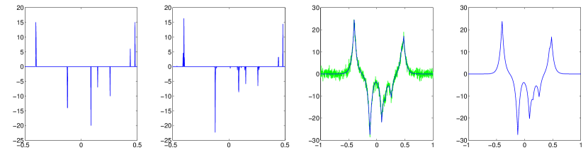
Figure 1: Deconvolution problem with penalty $R(x)=\|x\|_{l^{1}}$. From left to right: exact solution, reconstruction, exact (blue) and given (green) data, reconstructed data

This sparsity constraint is modeled by setting $R(x)=\|x\|_{l^{1}}$ in (3). Moreover, as instead of the exact data $y^{\dagger}$, only data $y^{\delta}$ perturbed by 18 % normal distributed noise is given, we choose $S(y^{\delta};y)=\frac{1}{2}\|y^{\delta}-y\|_{l^{2}}^{2}$ as data fidelity functional. According to the properties of the problem, $X=l^{r}\left(I_{X}\right),$ with $r\in(1,2]$ and $Y=l^{2}(I_{Y})$, seems to be a good choice. Here, $I_{X}=\left\{-\frac{1}{2},-\frac{1}{2}+\frac{1}{N-1},...,\frac{1}{2}\right\}$ is the discretization of $\left[\frac{1}{2},\frac{1}{2}\right]$ and $I_{Y}=\left\{-1,-1+\frac{2}{N-1},...,1\right\}$ the of $\left[-1,1\right]$. The discretization of $T$ is the discrete convolution. Now, for $r=2,1.75,1.5,1.25$ and $\alpha=5$ we apply the version described in theorem (3) of our algorithm to (3). Inspired by the optimality condition $T\bar{x}\in\partial g^{*}(\bar{p})$ with $g^{*}(p)=S(y^{\delta};p)^{*}=\frac{1}{2}\|p\|_{l^{2}(I_{Y})}^{2}+\left<y^{\delta},p\right>_{l^{2}}$, we pick

$$Tx_{0}\in\partial g^{*}(p_{0})=p_{0}+y^{\delta}\Leftrightarrow p_{0}=Tx_{0}-y^{\delta}$$ (44)

and $x_{0}=0$ as an initial guess. The generalized resolvents are given by (39) and example 11. Figure 2 shows that for experimental optimal chosen parameters $\sigma,\tau$ (according to Remark 8), we obtain faster convergence if $r$ turns 1. As Table 1 illustrates, this holds not only for the optimal parameter choice but also for any other choice of $\sigma$. Here, we chose $\tau\in(\sigma^{-1}\|T\|^{-2}-2^{-6},\sigma^{-1}\|T\|^{-2})$ for the Hilbert space case $X=l^{2}(I_{X}),$ and $\tau\in\left[\sigma^{-1}\|T\|^{-2}C_{1},\sigma^{-1}\|T\|^{-2}C_{2}\right],$ with $C_{1}=0.89,\ C_{2}=0.96\in[0.25,1],$ for the Banach space case $X=l^{1.25}(I_{X})$ (cf. Remark 8). Thus, we conclude that a choice of $X,$ which reflects the properties of the problem best, may provide the fastest convergence.

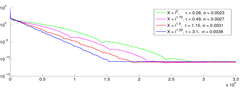
Figure 2: Convergence for the deconvolution problem with penalty $R(x)=\|x\|_{l^{1}}$. The error $\|x_{k}-x_{\alpha}\|_{l^{1}}$ of the iterates $(x_{k})_{k\in\mathbb{N}}$ generated by the algorithm $\text{CP-BS}1$ described in Theorem 3 is plotted over the iteration step $k$ for different choices of $X$. The parameters $\tau,\sigma$ are chosen optimally.

$\mathbf{\sigma}$	$0.007$		$0.0023\quad$		$0.00075$
$X=l^{2}(I_{X})$	76476	($\tau=0.0915$)	22368	($\tau=0.279$)	39418	($\tau=0.854$)
$X=l^{1.25}(I_{X})$	26271	($\tau=1.7$)	16575	($\tau=4.8$)	38710	($\tau=14.66$)

Table 1: Comparison of CP with $X=l^{2}(I_{X})$ and $\text{CP-BS}1$ with $X=l^{1.25}(I_{X})$ for the deconvolution problem with different choices of $\sigma$. The table shows the first iterations number $k$ for which $\|x_{\alpha}-x_{k}\|_{l^{1}}\leq 10^{-5}$, averaged over 100 experiments.

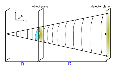
Figure 3: Experimental setup leading to the phase retrieval problem

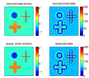
Figure 4: top: reconstructed phase $\phi$ and corresponding data $T(\phi)$ after 15 IRGN iterations; bottom: exact phase $\phi^{\dagger}$ and simulated Poisson distributed diffracton pattern $y^{\delta}$ with $\mathbb{E}[y^{\delta}]=T(\phi^{\dagger})$

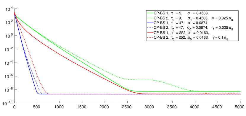
Figure 5: Convergence for the phase retrieval problem with penalty $R(x)=\frac{1}{2}\|x\|_{X}^{2}$ for $X=H^{1,1.1}(\mathbb{T}^{2})$ at Newton step $n=8$. The error $\|x_{n}-x_{k}\|_{X}$ of the iterates $(x_{k})_{k\in\mathbb{N}}$ of the algorithm CP-BS and the best approximation $x_{n}$ to the true minimizer of (4) is plotted over the iteration step $k$. The parameter choice rules are defined by Theorem 3 ($\text{CP-BS}1$, solid) and by Theorem 5 ($\text{CP-BS}2$, dotted), respectively. For given $\tau$ (or $\tau_{0}$), we set $\sigma=0.96\|T^{\prime}[\phi_{8}]\|^{-2}\tau^{-1}$ ($\sigma_{0}$ analogously)

As a second example, we consider a phase-retrieval problem (see figure 4): a sample of interest is illuminated by a coherent x-ray point source. From intensity measurements $\left|u^{\delta}(\cdot,D)\right|^{2}$ of the electric field $u:\mathbb{R}^{3}\to\mathbb{C}$, which are taken in the detector plane, orthogonal to the beam at a distance $D>0$, we want to retrieve information on the refractive index of the sample. More precisely, we are interested in the real phase $\phi:\mathbb{R}^{2}\times\left\{0\right\}\to\mathbb{R}$ of the object function $\mathcal{O}_{\phi}(x)=\exp\left(-\text{i}\kappa\phi(x)\right)$ describing the sample, where $\kappa$ denotes the wavenumber. We assume that $\text{e}^{-\text{i}\,\kappa D}\,u(\cdot,D)$ can be approximated by the so called Fresnel propagator $(P_{D}\mathcal{O})\coloneqq\mathcal{F}^{-1}\left(\chi_{-\frac{D}{\kappa}}\cdot(\mathcal{F}\mathcal{O})\right)$ where $\chi_{-c}(t_{1},t_{2}):=\exp\left(-\text{i}\,c\left(t_{1}^{2}+t_{2}^{2}\right)\right)$ is a chirp function with parameter $c>0$. Using the Fresnel scaling theorem we obtain the following forward operator $T$ mapping $\phi$ to $\left|u(\cdot,D)\right|^{2}$:

$$(T(\phi))(M\,t_{1},M\,t_{2})\coloneqq\frac{1}{M^{2}}\left|\left(P_{\frac{D}{M}}\mathcal{O}_{\phi}\right)\left(t_{1},t_{2}\right)\right|^{2}\,.$$

Here $M=\frac{R+D}{R}$, where $R>0$ is the distance between the sample and the source, denotes the geometrical magnification. For a detailed introduction to this problem and phase retrieval problems in general we refer to [20]. $T$ is Fréchet differentiable with

$$T^{\prime}[\phi](h)(M\,t_{1},M\,t_{2},D)=\frac{2}{M^{2}}\Re\left(\overline{P_{\frac{D}{M}}\left(\mathcal{O}(\phi)\right)(t_{1},t_{2})}\,\left(P_{\frac{D}{M}}\mathcal{O}^{\prime}_{\phi,h}\right)(t_{1},t_{2})\right)$$

so the IRNM (4) is applicable. This is an example with Poisson data, thus following [16, 33], after the discretization

$$x=\left(x_{j}\right)_{j\in\mathbb{T}^{2}_{N}}\coloneqq\phi(j_{1},j_{2})_{j\in\mathbb{T}^{2}_{N}},\quad y=\left(y_{j}\right)_{j\in M\mathbb{T}^{2}_{N}}\coloneqq|u(j_{1},j_{2},D)|^{2}_{j\in M\mathbb{T}^{2}_{N}}$$

we choose (using the convention $0\ln 0\coloneqq 0$):

$$S\left(y^{\delta};y\right)=\begin{cases}\sum\limits_{j\in M\mathbb{T}^{2}_{N}}y_{j}-y_{j}^{\delta}\ln y_{j}\quad&\text{if }y\geq 0\mbox{ and }y_{j}>0\mbox{ for all }j\mbox{ with }y^{\delta}_{j}>0\\ +\infty\quad&\text{otherwise}.\end{cases}$$

Moreover, motivated by the weighted least square approximation (cf. [27])

$$S\left(y^{\delta};y\right)\approx\frac{1}{2}\left\|\left(\frac{y_{j}^{\delta}-y_{j}}{\sqrt{y_{j}}}\right)_{j\in M\mathbb{T}_{N}^{2}}\right\|_{l^{2}}^{2},$$

in the $(n\!+\!1)$-th iteration step of the IRNM, we consider the weighted space $Y=l^{2}_{W}$ with weight $W\coloneqq\left(T(\phi_{n})+\epsilon\right)^{-1}$ and $\epsilon=0.1.$ Compared to setting $Y=l^{2}$, this leads to a faster convergence as numerical experiments show. $J_{l^{2}_{W}}\left(y\right)=W\,y,$ and $\partial S\left(y^{\delta};y\right)_{j}=1-\frac{y_{j}^{\delta}}{y_{j}}$ for $(y^{\delta},y)\in\text{dom }(S)=\left\{(y^{\delta},y)\,|\ S(y^{\delta};y)<+\infty\right\}$ imply

$$\left(\left(J_{l_{W}^{2}}\circ\partial S(y^{\delta},\cdot)+\sigma I\right)^{-1}(y)\right)_{j}=\frac{y_{j}-W_{j}^{-1}}{2\,\sigma}+\frac{\sqrt{\left(y_{j}-W_{j}^{-1}\right)^{2}+4\,\sigma\ W_{j}^{-1}\,y^{\delta}_{j}}}{2\sigma}.$$

Hence, we obtain the generalized resolvent $\left(\sigma\,\partial S(y^{\delta},\cdot)^{*}+I\right)^{-1}$ by Lemma 9. The ”blocky” structured solution is taken into account by setting $X:=H^{1,r}(\mathbb{T}^{2})$ with $r=1.1$ and $R(x)=\frac{1}{2}\|x\|_{X}^{2}.$ Note that although evaluating the generalized resolvent $(\tau\,\alpha R+J_{X})^{-1}=\frac{1}{\tau\,\alpha+1}J_{H^{-1,r^{*}}}=\frac{1}{\tau\,\alpha+1}\Lambda_{1}J_{l^{r^{*}}}\Lambda_{-1}$ is more expensive than in the case $X=l^{r}$, it does not increase the complexity of the algorithm as the evaluations of $T^{\prime}[\phi]$ and $T^{\prime}[\phi]^{*}$ include Fourier transforms as well. Since $R$ satisfies property (30), we can apply the variant $\text{CP-BS}1$ described in Theorem 3 and also the variant $\text{CP-BS}2$ given by Theorem 5. Figure 5 compares both versions in the $n=8$-th iteration step of the IRNM, where $\alpha=0.001$. The solid blue curve belongs to the version $\text{CP-BS}1$ for a optimal parameter choice of $\tau$ and $\sigma$ we found experimentally. Note that for the limit $\gamma\to 0$ the parameter choice rule of $\text{CP-BS}2$ coincide with the one of $\text{CP-BS}1$. In fact, choosing $\tau_{0}$ and $\sigma_{0}$ in the same way as $\tau$ and $\sigma$ that corresponds to this blue curve the version $\text{CP-BS}2$ with $\gamma=0.0025\alpha_{8}$ gives the same curve. Tuning also the parameters $\tau_{0},\sigma_{0}$ and $\gamma$ (reasonable large) in an optimal way, we did not obtain a better convergence result for $\text{CP-BS}2$ than for $\text{CP-BS}1$. However, $\text{CP-BS}2$ converges faster for $\tau=\tau_{0}$ sufficiently large and adequately chosen $\gamma$.

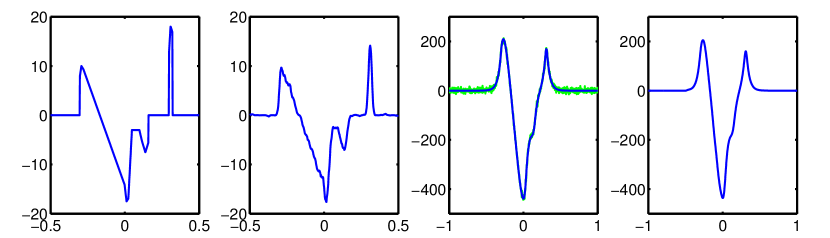
Figure 6: Deconvolution problem with penalty $R(x)=\frac{1}{2}\|x\|_{l^{1.5}}^{2}$. From left to right: exact solution, reconstruction, exact (blue) and given (green) data, reconstructed data

In our last example, we apply the version described by Theorem 6, which we denote as $\text{CP-BS}3$, to the Tikhonov functional

$$\frac{1}{2}\|Tx-y^{\delta}\|_{Y}^{2}+\frac{\alpha}{2}\|x\|_{X}^{2}$$

where $T$ is again the convolution operator (43). We set $\alpha=1$, $X=l^{1.5}(I_{X})$ and $Y=l^{2}(I_{X})$ (see figure 6). Setting $\mu=\frac{C\,\sqrt{\gamma\,\delta}}{2\|T\|}$ with $C=0.98,$ we obtain for any choice $\gamma=\delta\in(0,2]$ the fastest convergence rate. The same rate is also provided by $\text{CP-BS}1$ and $\text{CP-BS}2$ for optimal chosen (initial) parameter. Compared to the first example where more than 15000 iterations were required to satisfy the stopping criterion, here we only need 558 iterations.

References

[1]
R. Adams and J. Fournier.
Sobolev Spaces.
Pure and Applied Mathematics. Elsevier Science, 2003.
[2]
Y. I. Alber.
Generalized projection operators in Banach spaces: properties and
applications.
Functional Differential Equations, Proceedings of the Israel
Seminar in Ariel, 1:1–21, 1994.
[3]
E. Asplund.
Positivity of duality mappings.
Bulletin of the American Mathematical Society, 73(2):200–203,
03 1967.
[4]
V. Barbu and T. Precupanu.
Convexity and Optimization in Banach Spaces.
Mathematics and Its Applications (East European Series).
Bucureşti: D. Reidel Publishing Company, 1986.
[5]
H. H. Bauschke, X. Wang, and L. Yao.
General resolvents for monotone operators: characterization and
extension, biomedical mathematics: Promising directions.
In in Imaging, Therapy Planning and Inverse Problems, Medical
Physics Publishing, pages 57–74, 2010.
[6]
A. Beck and M. Teboulle.
A fast iterative shrinkage-thresholding algorithm for linear inverse
problems.
SIAM J. Img. Sci., 2(1):183–202, Mar. 2009.
[7]
R. I. Boţ, E. R. Csetnek, and A. Heinrich.
On the convergence rate improvement of a primal-dual splitting
algorithm for solving monotone inclusion problems.
arXiv:1303.2875, 2013.
[8]
T. Bonesky, K. S. Kazimierski, P. Maass, F. Schöpfer, and T. Schuster.
Minimization of Tikhonov functionals in Banach spaces.
Abstract and Applied Analysis, 2008.
[9]
D. W. Boyd.
The power method for norms.
Linear Algebra and its Applications, 9:95–101, 1974.
[10]
S. Boyd, N. Parikh, E. Chu, B. Peleato, and J. Eckstein.
Distributed optimization and statistical learning via the alternating
direction method of multipliers.
Foundations and Trends in Machine Learning, 3(1):1–122, 2011.
[11]
A. Chambolle and T. Pock.
A first-order primal-dual algorithm for convex problems with
applications to imaging.
J. Math. Imaging Vis., 40(1):120–145, May 2011.
[12]
I. Cioranescu.
Geometry of Banach Spaces, Duality Mappings and Nonlinear
Problems.
Mathematics and Its Applications. Springer, 1990.
[13]
P. L. Combettes and J.-C. Pesquet.
Proximal splitting methods in signal processing.
In Fixed-Point Algorithms for Inverse Problems in Science and
Engineering, pages 185–212. Springer, 2011.
[14]
O. Hanner.
On the uniform convexity of and .
Ark. Mat., 3:239–244, 1956.
[15]
B. He and X. Yuan.
Convergence analysis of primal-dual algorithms for a saddle-point
problem: From contraction perspective.
SIAM J. Img. Sci., 5(1):119–149, Jan. 2012.
[16]
T. Hohage and F. Werner.
Iteratively regularized Newton-type methods with general data
misfit functionals and applications to Poisson data.
Numerische Mathematik, 123(4):745–779, 2013.
[17]
B. Kaltenbacher and B. Hofmann.
Convergence rates for the iteratively regularized Gauss-Newton
method in Banach spaces.
Inverse Problems, 26:035007, 2010.
[18]
S. Kamimura and W. Takahashi.
Strong convergence of a proximal-type algorithm in a Banach space.
SIAM J. on Optimization, 13(3):938–945, 2002.
[19]
D. A. Lorenz and T. Pock.
An accelerated forward-backward algorithm for monotone inclusions.
CoRR, abs/1403.3522, 2014.
[20]
D. M. Paganin.
Coherent X-ray Optics.
Oxford Series on Synchrotron Radiation. New York: Oxford University
Press, 2006.
[21]
T. Pock and A. Chambolle.
Diagonal preconditioning for first order primal-dual algorithms in
convex optimization.
In Proceedings of the 2011 International Conference on Computer
Vision, ICCV ’11, pages 1762–1769, 2011.
[22]
R. Rockafellar.
On the maximal monotonicity of subdifferential mappings.
Pacific J. Math., 33(1):209–216, 1970.
[23]
R. Rockafellar.
Convex Analysis.
Princeton University Press, 1997.
[24]
L. I. Rudin, S. Osher, and E. Fatemi.
Nonlinear total variation based noise removal algorithms.
Phys. D, 60(1-4):259–268, Nov. 1992.
[25]
F. Schöpfer, A. K. Louis, and T. Schuster.
Nonlinear iterative methods for linear ill-posed problems in Banach
spaces.
Inverse Problems, 22(1):311–329, 2006.
[26]
T. Schuster, B. Kaltenbacher, B. Hofmann, and K. Kazimierski.
Regularization Methods in Banach Spaces, volume 10 of
Radon Series on Computational and Applied Mathematics.
De Gruyter, 2012.
[27]
R. Stück, M. Burger, and T. Hohage.
The iteratively regularized Gauss-Newton method with convex
constraints and applications in 4Pi-microscopy.
Inverse Problems, 28:015012, 2012.
[28]
M. Taylor.
Partial Differential Equations: Nonlinear Equations, volume 3.
Springer, New York, 1996.
[29]
R. Tibshirani.
Regression shrinkage and selection via the lasso.
Journal of the Royal Statistical Society, Series B,
58:267–288, 1994.
[30]
B. C. Vũ.
A splitting algorithm for dual monotone inclusions involving
cocoercive operators.
Advances in Computational Mathmatics, 38(3):667–681, 2013.
[31]
T. Valkonen.
A primal-dual hybrid gradient method for nonlinear operators with
applications to MRI.
Inverse Problems, 30(5):055012, 2014.
[32]
S. Villa, S. Salzo, L. Baldassarre, and A. Verri.
Accelerated and inexact forward-backward algorithms.
SIAM Journal on Optimization, 23(3):1607–1633, 2013.
[33]
F. Werner and T. Hohage.
Convergence rates in expectation for Tikhonov-type regularization
of inverse problems with Poisson data.
Inverse Problems, 28:104004, 2012.
[34]
Z.-B. Xu.
Characteristic inequalities of spaces and their applications.
Acta Math. Sinica, 32(2):209–218, 1989.
[35]
Z.-B. Xu and G. Roach.
Characteristic inequalities of uniformly convex and uniformly smooth
Banach spaces.
Journal of Mathematical Analysis and Applications,
157(1):189–210, 1991.
[36]
C. Zălinescu.
Convex analysis in general vector spaces.
River Edge, NJ : World Scientific, 2002.
Includes bibliographical references and index.