Sato-Tate groups of $y^{2}=x^{8}+c$ and $y^{2}=x^{7}-cx$.

Abstract.

We consider the distribution of normalized Frobenius traces for two families of genus 3 hyperelliptic curves over $\mathbb{Q}$ that have large automorphism groups: $y^{2}=x^{8}+c$ and $y^{2}=x^{7}-cx$ with $c\in\mathbb{Q}^{*}$. We give efficient algorithms to compute the trace of Frobenius for curves in these families at primes of good reduction. Using data generated by these algorithms, we obtain a heuristic description of the Sato-Tate groups that arise, both generically and for particular values of $c$. We then prove that these heuristic descriptions are correct by explicitly computing the Sato-Tate groups via the correspondence between Sato-Tate groups and Galois endomorphism types.

1. Introduction

In this paper we consider two families of hyperelliptic curves over $\mathbb{Q}$:

$$C_{1}\colon y^{2}=x^{8}+c,\qquad C_{2}\colon y^{2}=x^{7}-cx.$$

For $c\in\mathbb{Q}^{*}$, these equations define hyperelliptic curves of genus 3 with good reduction at primes $p>3$ for which $v_{p}(c)=0$ (in fact, $C_{1}$ also has good reduction at $3$). For each such $p$ we have the trace of Frobenius

$$t_{p}(C_{i}):=p+1-\#\overline{C}_{i}(\mathbb{F}_{p}),$$

where $\overline{C}_{i}$ denotes the reduction of $C_{i}$ modulo $p$. From the Weil bounds, we know that $t_{p}$ lies in the interval $[-6\sqrt{p},6\sqrt{p}]$. We wish to study the distribution of normalized Frobenius traces $t_{p}/\sqrt{p}\in[-6,6]$, as $p$ varies over primes of good reduction up to a bound $N$.

The generalized Sato-Tate conjecture predicts that as $N\to\infty$ this distribution converges to the distribution of traces in the Sato-Tate group, a compact subgroup of ${\rm USp}(6)$ associated to the Jacobian of the curve. For the two families considered here, the curves $C_{i}$ have Jacobians that are $\mathbb{Q}$-isogenous to the product of an elliptic curve and an abelian surface. This allows us to apply the classification of Sato-Tate groups for abelian surfaces obtained in [FKRS12] to determine the Sato-Tate groups that arise. This is achieved in §5.

After recalling the definition of the Sato-Tate group of an abelian variety in §2, we begin in §3 by deriving formulas for the Frobenius trace $t_{p}(C_{i})$ in terms of the Hasse-Witt matrix of $\overline{C}_{i}$. These formulas allow us to design particularly efficient algorithms for computing $t_{p}(C_{i})$. In §4, under the assumption of the Sato-Tate conjecture, we use the numerical data obtained by applying these algorithms to heuristically guess the isomorphism class of the Sato-Tate groups of $C_{1}$ and $C_{2}$. The explicit computation in §5 proves that, in fact, these guesses are correct, without appealing to the Sato-Tate conjecture.

Strictly speaking, §4 and §5 are independent of each other. However, we should emphasize that in the process of achieving our results, there was a constant and mutually beneficial interplay between the two distinct approaches.

Up to dimension 3, the Sato-Tate group of an abelian variety defined over a number field $k$ is determined by its ring of endomorphisms over an algebraic closure of $k$. Although the Sato-Tate group does not capture the ring structure of the endomorphisms, it does codify the $\mathbb{R}$-algebra generated by the endomorphism ring, and the structure of this $\mathbb{R}$-algebra as a Galois module, what we refer to as the Galois endomorphism type of the abelian variety. As an example, in §6 we compute the Galois endomorphism type of the Jacobian of $C_{2}$.

The problem of analysing the Frobenius trace distributions and determining the Sato-Tate groups that arise in these two families was originally posed as part of a course given by the authors at the winter school Frobenius Distributions on Curves held in February, 2014, at the Centre International de Rencontres Mathématiques in Luminy. This problem turned out to be more challenging than we anticipated (the analogous question in genus $2$ is quite straight-forward); this article represents a solution.

1.1. Acknowledgements

Both authors are grateful to the Centre International de Rencontres Mathématiques for the hospitality and financial support provided, and to the anonymous referee.

2. Background

We start by briefly recalling the definition of the Sato-Tate group of an abelian variety $A$ defined over a number field $k$, and set some notation. For a more detailed presentation we refer to [Ser12, Chap. 8] or [FKRS12, §2].

2.1. The Sato-Tate group of an abelian variety

Let $\overline{k}$ denote a fixed algebraic closure of $k$, and let $g$ be the dimension of $A$. For each prime $\ell$ we have a continuous homomorphism

$$\varrho_{A,\ell}\colon{\rm Gal}(\overline{k}/k)\rightarrow{\rm GSp}_{2g}(\mathbb{Q}_{\ell})$$

arising from the action of ${\rm Gal}(\overline{k}/k)$ on the rational Tate module $(\varprojlim A[\ell^{n}])\otimes\mathbb{Q}$. Here ${\rm GSp}$ denotes the group of symplectic similitudes, which preserve a symplectic form up to a scalar; in our setting the preserved symplectic form arises from the Weil pairing. Let $G_{\ell}$ be the Zariski closure of the image of $\varrho_{A,\ell}$, and let $G_{\ell}^{1}$ be the kernel of the similitude character $G_{\ell}\rightarrow\mathbb{Q}_{\ell}^{*}$. We now choose an embedding $\iota\colon\mathbb{Q}_{\ell}\hookrightarrow\mathbb{C}$, and for each prime ideal $\mathfrak{p}$ of the ring of integers of $k$, let ${\rm Frob}_{\mathfrak{p}}$ denote an arithmetic Frobenius at $\mathfrak{p}$ and let $N(\mathfrak{p})$ be the cardinality of its residue field.

Definition 2.1.

The Sato-Tate group of $A$, denoted $\operatorname{ST}(A)$, is a maximal compact subgroup of $G_{\ell}^{1}\otimes_{\iota}\mathbb{C}$. For each prime $\mathfrak{p}$ of good reduction for $A$, let $s(\mathfrak{p}):=\varrho_{A,\ell}({\rm Frob}_{\mathfrak{p}})\otimes_{\iota}N(\mathfrak{p})^{-1/2}$.

Let ${\rm USp}(2g)$ denote the group of $2g\times 2g$ complex matrices that are unitary and preserve a fixed symplectic form; this is a real Lie group of dimension $g(2g+1)$. One can show that $\operatorname{ST}(A)$ is well-defined up to conjugacy in ${\rm USp}(2g)$, and that $s(\mathfrak{p})$ determines a conjugacy class in $\operatorname{ST}(A)$.

Conjecture 2.2 (generalized Sato-Tate).

Let $X$ denote the set of conjugacy classes of $\operatorname{ST}(A)$. Then:

1. The conjugacy class of $\operatorname{ST}(A)$ in ${\rm USp}(2g)$ and the conjugacy classes $s(\mathfrak{p})$ in $\operatorname{ST}(A)$ are independent of the choice of the prime $\ell$ and the embedding $\iota$.

2. When the primes $\mathfrak{p}$ are ordered by norm, the $s(\mathfrak{p})$ are equidistributed on $X$ with respect to the projection of the Haar measure of $\operatorname{ST}(A)$ on $X$.

It follows from [BK15] that part $(i)$ of the above conjecture is true for $g\leq 3$. We next summarize some basic properties of the Sato-Tate group that we will need in our forthcoming discussion. If $L/k$ is a field extension, we write $A_{L}$ for the base change of $A$ to $L$. We denote by $K_{A}$ the minimal extension $L/k$ over which all the endomorphisms of $A$ are defined, that is, the minimal extension for which ${\rm End}(A_{L})\simeq{\rm End}(A_{\bar{k}})$.

The Sato-Tate group $\operatorname{ST}(A)$ is a compact real Lie group, but it need not be connected. We use $\operatorname{ST}^{0}(A)$ to denote the connected component of the identity.

proposition 2.3 (Prop. 2.17 of [FKRS12]).

If $g\leq 3$, then the group of connected components $\operatorname{ST}(A)/\operatorname{ST}^{0}(A)$ is isomorphic to ${\rm Gal}(K_{A}/k)$.

This proposition implies, in particular, that a prime $\mathfrak{p}$ of good reduction for $A$ splits completely in $K_{A}$ if and only if $s(\mathfrak{p})\in\operatorname{ST}^{0}(A)$. One can in fact show a little bit more: for any algebraic extension $L/k$, the Sato-Tate group $\operatorname{ST}(A_{L})$ is a subgroup of $\operatorname{ST}(A)$ with $\operatorname{ST}^{0}(A_{L})=\operatorname{ST}^{0}(A)$ and

$$\operatorname{ST}(A_{L})/\operatorname{ST}^{0}(A_{L})\simeq{\rm Gal}(K_{A}/(K_{A}\cap L))\subseteq{\rm Gal}(K_{A}/k).$$

2.2. Galois endomorphism types

We now work in the category $\mathcal{C}$ of pairs $(G,E)$, where $G$ is a finite group and $E$ is an $\mathbb{R}$-algebra equipped with an $\mathbb{R}$-linear action of $G$. A morphism $\Phi\colon(G,E)\rightarrow(G^{\prime},E^{\prime})$ of $\mathcal{C}$ consists of a pair $\Phi:=(\phi_{1},\phi_{2})$, where $\phi_{1}\colon G\rightarrow G^{\prime}$ is a morphism of groups and $\phi_{2}\colon E\rightarrow E^{\prime}$ is an equivariant morphism of $\mathbb{R}$-algebras, that is,

$$\phi_{2}(\phi_{1}(g)e)=\phi_{2}(g)(\phi_{1}(e))\qquad\text{for all $g\in G$ and $e\in E$.}$$

Definition 2.4.

The Galois endomorphism type of $A$ is the isomorphism class in $\mathcal{C}$ of the pair $({\rm Gal}(K_{A}/k),{\rm End}(A_{K_{A}})\otimes_{\mathbb{Z}}\mathbb{R})$.

By [FKRS12, Prop. 2.19], for $g\leq 3$, the Galois endomorphism type is determined by the Sato-Tate group (in fact, the proof of this statement is effective, as we will illustrate in §6). This result admits a converse statement at least for $g\leq 2$.

Theorem 2.5 (Thm. 4.3 of [FKRS12]).

For fixed $g\leq 2$, the Sato-Tate group and the Galois endomorphism type of an abelian variety $A$ defined over a number field $k$ uniquely determine each other. For $g=1$ (resp. $g=2$) there are $3$ (resp. $52$) possibilities for the Galois endomorphism type, all of which arise for some choice of $A$ and $k$.

For $g=1$ the $3$ possible Sato-Tate groups are ${\rm SU}(2)={\rm USp}(2)$, a copy of the unitary group ${\rm U}(1)$ embedded in ${\rm SU}(2)$, and its normalizer in ${\rm SU}(2)$; these arise, respectively, for elliptic curves $E/k$ without CM, with CM by a field contained in $k$, and with CM by a field not contained in $k$. For $g=2$ a complete list of the $52$ possible Sato-Tate groups can be found in [FKRS12].

In order to simplify the notation, when $C$ is a smooth projective curve defined over the number field $k$, we may simply write

$$\operatorname{ST}(C):=\operatorname{ST}(\operatorname{Jac}(C)),\qquad\operatorname{ST}^{0}(C):=\operatorname{ST}^{0}(\operatorname{Jac}(C)),\qquad{\text{and}}\qquad K_{C}:=K_{\operatorname{Jac}(C)}\,.$$

3. Trace formulas

Let $\overline{C}/\mathbb{F}_{p}$ be a smooth projective curve of genus $g\geq 1$ defined by an equation of the form $y^{2}=f(x)$ with $f\in\mathbb{F}_{p}[x]$ squarefree. Let $n=(p-1)/2$ and let $f_{k}^{n}$ denote the coefficient of $x^{k}$ in the polynomial $f(x)^{n}$. The Hasse–Witt matrix of $\overline{C}$ is the $g\times g$ matrix $W_{p}:=[w_{ij}]$ over $\mathbb{F}_{p}$, where

$$w_{ij}:=f^{n}_{ip-j}\qquad(1\leq i,j\leq g).$$

It is shown in [Man61, Yui78] that the characteristic polynomial $\chi(\lambda)$ of the Frobenius endomorphism of $\operatorname{Jac}(\overline{C})$ satisfies

$$\chi(\lambda)\equiv(-1)^{g}\lambda^{g}\det(W_{p}-\lambda I)\bmod p.$$

In particular,

$$\operatorname{tr}W_{p}\equiv t_{p}\bmod p,$$

where $t_{p}:=p+1-\#\overline{C}(\mathbb{F}_{p})$ is the trace of Frobenius. The Weil bounds imply $|t_{p}|\leq 2g\sqrt{p}$, which means that for all $p\geq 16g^{2}$, the trace of $W_{p}$ uniquely determines the integer $t_{p}$.

Let us now specialize to the case where $f(x)$ has the form

$$f(x)=ax^{d}+bx^{e},$$

with $d\in\{2g+1,2g+2\}$, $e\in\{0,1\}$, and $a,b\in\mathbb{F}_{p}^{*}$; this includes the families $C_{i}$ defined in §1. Writing

$$f(x)^{n}=x^{en}(ax^{d-e}+b)^{n}$$

and applying the binomial theorem yields

$$f^{n}_{en+(d-e)r}=\binom{n}{r}a^{r}b^{n-r},$$

and we have $f^{n}_{k}=0$ whenever $k$ is not of the form $k=en+(d-e)r$. Setting $k=ip-j=i(2n+1)-j$ and solving for $r=r_{ij}$ yields

$$r_{ij}:=\frac{(2i-e)n+i-j}{d-e}\qquad(1\leq i,j\leq g).$$

The entries of the Hasse-Witt matrix for $y^{2}=ax^{d}+bx^{e}$ are thus given by

(1) $$w_{ij}=\begin{cases}\binom{n}{r_{ij}}a^{r_{ij}}b^{n-r_{ij}}&\text{if }r_{ij}\in\mathbb{Z},\\ 0&\text{otherwise}.\end{cases}$$

For any fixed integer $i\in[1,g]$, the quantity $(2i-e)n+i-j$ lies in an interval of width $g-1<(d-e)/2$, as $j$ varies over integers in $[1,g]$. This implies that at most one entry $w_{ij}$ in each row of $W_{p}$ is nonzero, and for this entry $r_{ij}$ is simply the nearest integer to $(2i-e)n/(d-e)$.

We now specialize to the two families of interest and assume $p>3$. For $C_{1}\colon y^{2}=x^{8}+c$ we have $d=8,e=0,a=1$, and $b=\overline{c}$, where $\overline{c}$ denotes the image of $c$ in $\mathbb{F}_{p}$. We thus have

$$r_{ij}=\frac{2in+i-j}{8}=\frac{ip-j}{8}.$$

For integers $i,j\in[1,3]$, the integral values of $r_{ij}$ that arise are listed below:

$p\equiv 1\bmod 8:$	$r_{11}=\frac{n}{4},$	$r_{22}=\frac{n}{2},$	$r_{33}=\frac{3n}{4}$;
$p\equiv 3\bmod 8:$	$r_{13}=\frac{n-1}{4},$	$r_{31}=\frac{3n+1}{4}$;
$p\equiv 5\bmod 8:$	$r_{22}=\frac{n}{2}$;
$p\equiv 7\bmod 8:$	none.

This yields the following formulas for the trace of Frobenius:

(2) $$t_{p}(C_{1})\equiv_{p}\begin{cases}\binom{n}{n/2}\overline{c}^{n/2}+\binom{n}{n/4}\overline{c}^{n/4}+\binom{n}{n/4}\overline{c}^{3n/4}&\text{if }p\equiv 1\bmod 8,\\ \binom{n}{n/2}\overline{c}^{n/2}&\text{if }p\equiv 5\bmod 8,\\ 0&\text{otherwise}.\\ \end{cases}$$

For $C_{2}\colon y^{2}=x^{7}-cx$ we have $d=7,e=1,a=1$, and $b=-\overline{c}$. We thus have

$$r_{ij}=\frac{(2i-1)n+i-j}{6}.$$

For integers $i,j\in[1,3]$, the integral values of $r_{ij}$ that arise are listed below:

$p\equiv 1\bmod 12:$	$r_{11}=\frac{n}{6},$	$r_{22}=\frac{n}{2},$	$r_{33}=\frac{5n}{6}$;
$p\equiv 5\bmod 12:$	$r_{13}=\frac{n-2}{6},$	$r_{22}=\frac{n}{2}$,	$r_{31}=\frac{5n+2}{6}$;
$p\equiv 7\bmod 12:$	none;
$p\equiv 11\bmod 12:$	none.

This yields the following formulas for the trace of Frobenius:

(3) $$t_{p}(C_{2})\equiv_{p}\begin{cases}\binom{n}{n/2}(-\overline{c})^{n/2}+\binom{n}{n/6}(-\overline{c})^{n/6}+\binom{n}{n/6}(-\overline{c})^{5n/6}&\text{if }p\equiv 1\bmod 12,\\ \binom{n}{n/2}(-\overline{c})^{n/2}&\text{if }p\equiv 5\bmod 12,\\ 0&\text{otherwise}.\\ \end{cases}$$

3.1. Algorithms

Computing the powers of $\overline{c}$ that appear in the formulas (2) and (3) for $t_{p}(C_{i})$ is straight-forward; using binary exponentiation this requires just $O(\log p)$ multiplication in $\mathbb{F}_{p}$. The only potential difficulty is the computation of the binomial coefficients $\binom{n}{n/2},\binom{n}{n/4},\binom{n}{n/6}$ modulo $p$, where $n=(p-1)/2$ and $p$ is known to lie in a suitable residue class. Fortunately, there are very efficient formulas for computing these particular binomial coefficients modulo suitable primes $p$. These are given by the lemmas below, in which $(\frac{2}{p})\in\{\pm 1\}$ denotes the Legendre symbol, and $m$, $x$, and $y$ denote integers.

Lemma 3.1.

Let $p=4m+1=x^{2}+y^{2}$ be prime, with $x\equiv-\bigl{(}\frac{2}{p}\bigr{)}\bmod 4$. Then

$$\binom{2m}{m}\equiv 2(-1)^{m+1}x\bmod p.$$

Proof.

See [BEW98, Thm. 9.2.2]. ∎

Lemma 3.2.

Let $p=8m+1=x^{2}+2y^{2}$ be prime, with $x\equiv-\bigl{(}\frac{2}{p}\bigr{)}\bmod 4$. Then

$$\binom{4m}{m}\equiv 2(-1)^{m+1}x\bmod p.$$

Proof.

See [BEW98, Thm. 9.2.8]. ∎

Lemma 3.3.

Let $p=12m+1=x^{2}+y^{2}$ be prime, with $x\equiv-\bigl{(}\frac{2}{p}\bigr{)}\bmod 4$, and define $\epsilon$ to be $0$ if $x\equiv 0\bmod 3$ and $1$ otherwise. Then

$$\binom{6m}{m}\equiv 2(-1)^{m+\epsilon}x\bmod p.$$

Proof.

See [BEW98, Thm. 9.2.10] (replace $\rho_{4}^{2}$ with $(-1)^{\epsilon-1}$). ∎

To apply these lemmas, one uses Cornacchia’s algorithm to find a solution $(x,y)$ to $p=x^{2}+dy^{2}$, where $d=1$ when computing $\binom{n}{n/2}\bmod p$ or $\binom{n}{n/6}\bmod p$, and $d=2$ when computing $\binom{n}{n/4}$. Cornacchia’s algorithm requires as input a square-root $\delta$ of $-d$ modulo $p$ (if no such $\delta$ exists then $p=x^{2}+dy^{2}$ has no solutions).

Cornacchia’s Algorithm
Given integers $1\leq d<m$ and an integer $\delta\in[0,m/2]$ such that $\delta^{2}\equiv-d\bmod m$, find a solution $(x,y)$ to $x^{2}+dy^{2}=m$ or determine that none exist as follows:

1. Set $x_{0}:=m$, $x_{1}:=\delta$, and $i=1$.

2. While $x_{i}^{2}\geq m$, set $x_{i+1}:=x_{i-1}\bmod x_{i}$ with $x_{i+1}\in[0,x_{i})$ and increment $i$.

3. If $(m-x_{i}^{2})/d=y^{2}$ for some $y\in\mathbb{Z}$, output the solution $(x_{i},y)$.
   Otherwise, report that no solution exists.

See [Bas04] for a simple proof of the correctness of this algorithm. We now consider its computational complexity, using $\operatorname{\mathsf{M}}(n)$ to denote the time to multiply two $n$-bit integers; we may take $\operatorname{\mathsf{M}}(n)=O(n\log n\log\log n)$ via [SS71]. The first two steps correspond to half of the standard Euclidean algorithm for computing the GCD of $m$ and $\delta$, whose bit-complexity is bounded by $O(\log^{2}m)$; see [GG13, Thm. 3.13]. The time required in step 3 to perform a division and check whether the result is a square integer is also $O(\operatorname{\mathsf{M}}(\log m))$; see [GG13, Thm. 9.8, Thm. 9.28]). Thus the overall complexity is $O(\log^{2}m)$, the same as the Euclidean algorithm.

Remark 3.4.

There is an asymptotically faster version of the Euclidean algorithm that allows one to compute any particular pair of remainders $(x_{i-1},x_{i})$, including the unique pair for which $x_{i-1}\geq\sqrt{m}>x_{i}$, in $O(\operatorname{\mathsf{M}}(\log m)\log\log m)$ time; see [PW03]. This yields a faster version of Cornacchia’s algorithm that runs in quasi-linear time, but we will not use this.

We now turn to the problem of computing the square-root $\delta$ of $-d\bmod m$ that is required by Cornacchia’s algorithm. There are two basic strategies for doing this:

1. (Cipolla-Lehmer) Use a probabilistic root-finding algorithm to factor $x^{2}+d$ in $\mathbb{F}_{p}[x]$. This takes $O(\operatorname{\mathsf{M}}(\log p)\log p)$ expected time.

2. (Tonelli-Shanks) Given a generator $g$ for the 2-Sylow subgroup of $\mathbb{F}_{p}^{*}$, compute the discrete logarithm $e$ of $(-d)^{s}\in\langle g\rangle$ and let $\delta=g^{-e/2}(-d)^{(s+1)/2},$ where $p=2^{v}s+1$ with $s$ odd. This takes $O(\operatorname{\mathsf{M}}(\log p)(\log p+v\log v/\log\log v))$ time if the algorithm in [Sut11] is used to compute the discrete logarithm.

We will exploit both approaches. To obtain a generator for the 2-Sylow subgroup of $\mathbb{F}_{p}^{*}$ one may take $\alpha^{s}$ for any quadratic non-residue $\alpha$. Half the elements of $\mathbb{F}_{p}^{*}$ are non-residues, so randomly selecting elements and computing Legendre symbols will yield a non-residue after 2 attempts, on average, and each attempt takes $O(\operatorname{\mathsf{M}}(\log p)\log\log p)$ time, via [BZ10]. Unfortunately, we know of no efficient way to deterministically obtain a quadratic non-residue modulo $p$ without assuming the generalized Riemann hypothesis (GRH). Under the GRH the least non-residue is $O((\log p)^{2})$ [Bac90], thus if we simply test increasing integers $2,3,\ldots$ we can obtain a non-residue $\alpha$ for a total cost of $O(\operatorname{\mathsf{M}}(\log p)\log^{2}p\log\log p)$.

But we are actually interested in computing $t_{p}(C_{i})$ for many primes $p\leq N$, for some large bound $N$; on average, this approach will find a non-residue very quickly. As $N\to\infty$ the average value of the least non-residue converges to

$$\sum_{k=1}^{\infty}\frac{p_{k}}{2^{k}}=3.674643966\ldots,$$

where $p_{k}$ denotes the $k$th prime, as shown by Erdös [Erd61].

Finally, we should mention an alternative approach to solving $p=x^{2}+dy^{2}$ that is completely deterministic. Construct an elliptic curve $E/\mathbb{F}_{p}$ with complex multiplication by the imaginary quadratic order $\mathcal{O}$ with discriminant $D=-d$ (or $D=-4d$ if $-d\not\equiv 0,1\bmod 4$) and then use Schoof’s algorithm [Sch85] to compute the trace of Frobenius $t$ of $E$. We then have $4p=t^{2}-v^{2}D$, since the Frobenius endomorphism with trace $t$ and norm $p$ corresponds to $\frac{t\pm v\sqrt{D}}{2}\in\mathcal{O}$, and therefore $(t/v)^{2}\equiv D\bmod p$. If $D=-d$, we have a square root of $-d$ modulo $p$ and can use Cornacchia’s algorithm to solve $p=x^{2}+dy^{2}$. If $D=-4d$, then $t$ is even and $(t/2,2v)$ is already a solution to $p=x^{2}+dy^{2}$. We are specifically interested in the cases $D=-4$ and $D=-8$. For $D=-4$ we can take $E\colon y^{2}=x^{3}-x$, and for $D=-8$ we can take $E\colon y^{2}=x^{4}+4x^{2}+2x$; see §3 of Appendix A in [Sil94].

We collect all of these observations in the following theorem.

Theorem 3.5.

Let $C_{1}\colon y^{2}=x^{8}+c$ and $C_{2}\colon y^{2}=x^{7}-cx$ be as above. Let $p>3$ be a prime with $v_{p}(c)=0$. We can compute $t_{p}(C_{i})$:

• probabilistically in $O(\operatorname{\mathsf{M}}(\log p)\log p)$ expected time;

• deterministically in $O(\operatorname{\mathsf{M}}(\log p)\log^{2}p\log\log p)$ time, assuming GRH;

• deterministically in $O(\operatorname{\mathsf{M}}(\log^{3}p)\log^{2}p/\log\log p)$ time.

For any positive integer $N$, we can compute $t_{p}(C_{i})$ for all $3<p\leq N$ with $v_{p}(c)=0$ deterministically in $O(N\operatorname{\mathsf{M}}(\log N))$ time.

Proof.

Since we are computing asymptotic bounds, we may assume $p\geq 144$ (if not, just count points naïvely). Then $t_{p}(C_{i})\bmod p$ uniquely determines $t_{p}(C_{i})\in\mathbb{Z}$.

For the first bound we use the Cipolla-Lehmer approach to probabilistically compute the square root required by Cornacchia’s algorithm in $O(\operatorname{\mathsf{M}}(\log p)\log p)$ time, matching the time required to apply any of Lemmas 2.1-4, and the time required by the exponentiations of $\overline{c}$ needed to compute $t_{p}(C_{i})$.

For the second bound we instead use the Tonelli-Shanks approach to computing square roots, relying on iteratively testing increasing integers to find a non-residue. Under the GRH this takes $O(\operatorname{\mathsf{M}}(\log p)\log^{2}p\log\log p)$ time, which dominates everything else.

For the third bound, we instead use Schoof’s approach to solve $p=x^{2}+dy^{2}$. The analysis in [SS14, Cor. 11] shows that Schoof’s algorithm can be implemented to run in $O(\operatorname{\mathsf{M}}(\log^{3}p)\log^{2}p/\log\log p)$ time.

For the final bound we proceed as in the GRH bound but instead rely on the Erdös bound for the least non-residue modulo $p\leq N$, on average. By the prime number theorem there are $O(N/\log N)$ primes $p\leq N$; the total number of quadratic residue tests is thus $O(N/\log N)$. It takes $O(\operatorname{\mathsf{M}}(\log N)\log\log N)$ time for each test, so the total time spent finding non-residues is $O(N\operatorname{\mathsf{M}}(\log N)\log\log N/\log N)$. The average $2$-adic valuation of $p-1$ over primes $p\leq N$ is $O(1)$, so the total time spent computing square roots modulo primes $p\leq N$ using the Tonelli-Shanks approach is $O((N/\log N)\operatorname{\mathsf{M}}(\log N)\log N))=O(N\operatorname{\mathsf{M}}(\log N))$ which dominates the time spent finding non-residues and matches the time spent on everything else. ∎

We note that the average time per prime $p\leq N$ using a deterministic algorithm is $O(\operatorname{\mathsf{M}}(\log p)\log p)$, which matches the expected time when applying our probabilistic approach for any particular prime $p\leq N$; both bounds are quasi-quadratic $O((\log p)^{2+o(1)})$. For comparison, the average time per prime $p\leq N$ achieved using the average polynomial time algorithm in [HS14a, HS14b] is $O((\log p)^{4+o(1)})$.

Remark 3.6.

Although Theorem 3.5 only addresses the computation of $t_{p}(C_{i})$, for $p\not\equiv 3\bmod 8$ (resp. $p\not\equiv 5\bmod 12$) we can readily compute the entire Hasse-Witt matrix $W_{p}$ for $C_{1}$ (resp. $C_{2}$) using the same approach and within the same complexity bounds.

4. Guessing Sato-Tate groups

In this section we analyze the Sato-Tate distributions of the curves $C_{i}$ and arrive at a heuristic characterization of their Sato-Tate groups up to isomorphism, based on statistics collected using the algorithm described in §3.1. In §5 we will unconditionally prove that our heuristic characterizations are correct.

4.1. The Sato-Tate distribution of $C_{1}$

Before applying any heuristics we can derive some information about the structure of the Sato-Tate group directly from the formulas developed in the previous section. The possible shapes of the Hasse-Witt matrix for $C_{1}$ at a primes $p\equiv 1,3,5,7\bmod 8$ are depicted below, with the residue class of $p\bmod 8$ in parentheses:

$$\begin{bmatrix}*&0&0\\ 0&*&0\\ 0&0&*\end{bmatrix}(1),\quad\begin{bmatrix}0&0&*\\ 0&0&0\\ *&0&0\end{bmatrix}(3),\quad\begin{bmatrix}0&0&0\\ 0&*&0\\ 0&0&0\end{bmatrix}(5),\quad\begin{bmatrix}0&0&0\\ 0&0&0\\ 0&0&0\end{bmatrix}(7).$$

From this we can (unconditionally) conclude the following:

1. the component group $\operatorname{ST}(C_{1})/\operatorname{ST}^{0}(C_{1})$ has order divisible by $4$;

2. we have $s(p)$ in $\operatorname{ST}^{0}(C_{1})$ only if $p\equiv 1\bmod 8$;

3. the field $K_{C_{1}}$ contains $\mathbb{Q}(i,\sqrt{2})$.

We note that (c) follows immediately from (b): a prime $p>2$ splits completely in $\mathbb{Q}(i,\sqrt{2})$ if and only if $p\equiv 1\bmod 8$.

Table 1 lists moment statistics $M_{n}$ for the curve $C_{1}\colon y^{2}=x^{8}+c$ for selected values of $c$, where $M_{n}$ is the average value of the $n$th power of the normalized $L$-polynomial coefficient

$$a_{1}:=-t_{p}/\sqrt{p},$$

over odd primes $p\leq 2^{40}$ not dividing $c$. The moment statistics $M_{n}$ for odd $n$ are all close to zero, so we list $M_{n}$ only for even $n$.

$c$	$M_{2}$	$M_{4}$	$M_{6}$	$M_{8}$	$M_{10}$
$1$	3.000	50.999	1229.971	33634.058	978107.050
$2$	2.000	27.000	619.987	16834.560	489116.939
$3$	2.000	24.000	469.984	11234.520	297593.517
$4$	3.000	51.000	1229.990	33634.650	978125.742
$5$	2.000	23.999	469.976	11234.211	297585.653
$6$	2.000	23.999	469.979	11234.275	297587.173
$7$	2.000	23.999	469.968	11234.007	297579.866
$8$	2.000	27.000	619.987	16834.560	498116.939
$9$	2.000	27.000	619.991	16834.654	498118.664
$2^{4}$	3.000	50.999	1229.971	33634.058	978107.050
$3^{3}$	2.000	24.000	469.987	11234.520	297594.971
$2^{5}$	2.000	27.000	619.987	16834.560	498116.939
$2^{6}$	3.000	51.000	1229.990	33634.650	978125.742
$3^{4}$	3.000	51.000	1229.990	33634.593	978121.494

Table 1. Trace moment statistics for $C_{1}\colon y^{2}=x^{8}+c$ for $p\leq 2^{40}$.

There appear to be three distinct trace distributions that arise, depending on whether the integer $c$ is in

$$\mathbb{Q}(i,\sqrt{2})^{*4},\quad\mathbb{Q}(i,\sqrt{2})^{*2}\setminus\mathbb{Q}(i,\sqrt{2})^{*4},\quad\text{or}\quad\mathbb{Q}(i,\sqrt{2})^{*}\setminus\mathbb{Q}(i,\sqrt{2})^{*2};$$

these can be distinguished by whether the nearest integer to $M_{4}$ is 51, 27, or 24, respectively. Histogram plots of representative examples are shown with $c=1,2,3$ in Figure 1. We note that in each histogram the central spike at $0$ has area 1/2, while the spikes at $-2$ and $2$ have area zero.

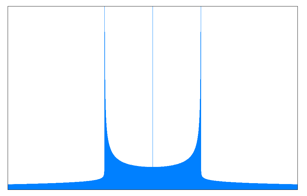
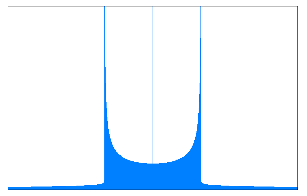
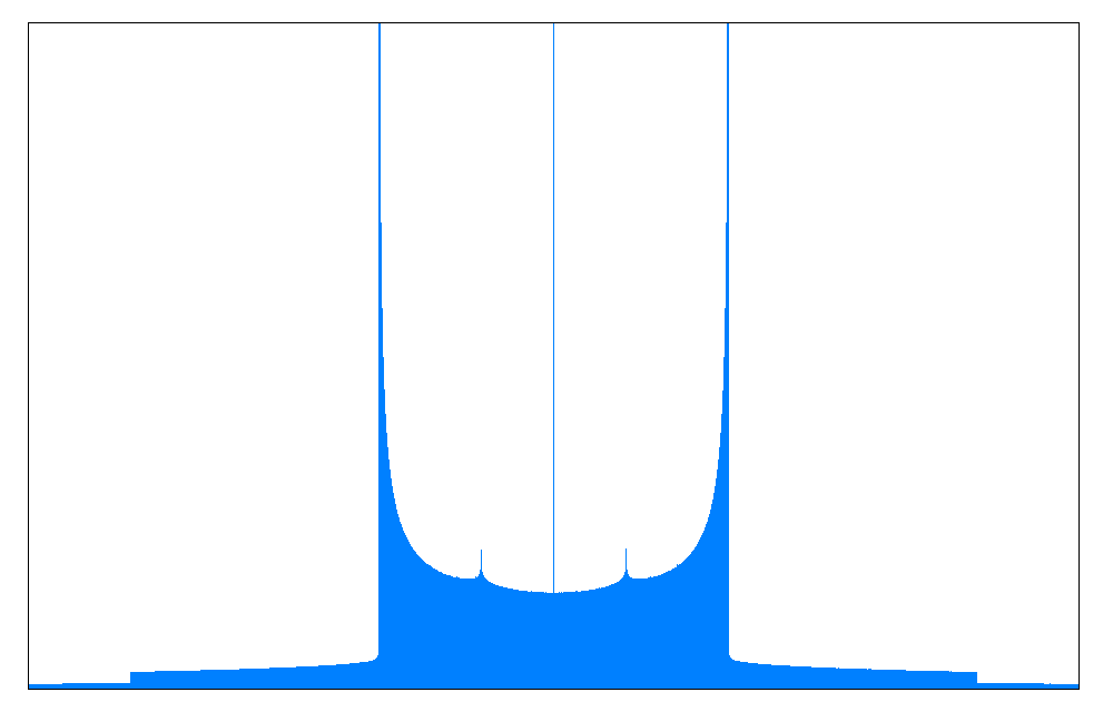
$y^{2}=x^{8}+1$                        $y^{2}=x^{8}+2$                        $y^{2}=x^{8}+3$

Figure 1. $a_{1}$-histograms for three representative curves $C_{1}$.

Based on the data in Table 1, we expect $K_{C_{1}}$ to contain $\mathbb{Q}(i,\sqrt{2},\sqrt[4]{c})$. If we now require $c$ to be a fourth-power and restrict to primes $p\equiv 1\bmod 8$, we can investigate the Sato-Tate distribution of $C_{1}$ over the number field $\mathbb{Q}(i,\sqrt{2},\sqrt[4]{c})$. For $c=1$ we obtain the moments listed below:

$c$	$M_{2}$	$M_{4}$	$M_{6}$	$M_{8}$	$M_{10}$
$1$	10.000	197.997	4899.892	134466.452	3912182.569

The corresponding histogram is shown in Figure 2.

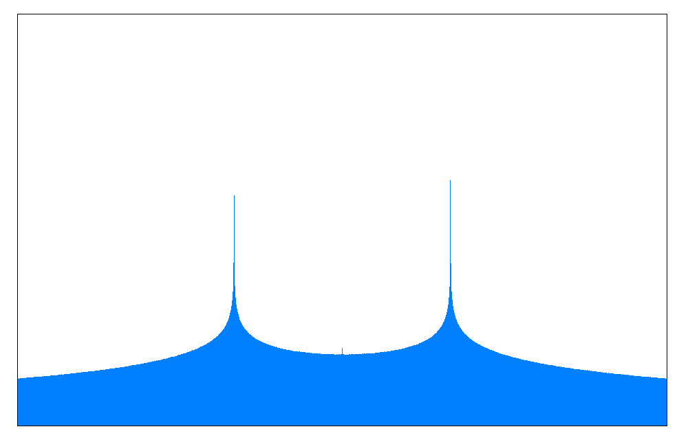
Figure 2. $a_{1}$-histogram for $y^{2}=x^{8}+1$ over $\mathbb{Q}(i,\sqrt{2})$.

We claim that this distribution corresponds to a connected Sato-Tate group, namely, the group

$${\rm U}(1)_{2}\times{\rm U}(1):=\left\langle\begin{bmatrix}U(u)&0&0\\ 0&U(u)&0\\ 0&0&U(v)\end{bmatrix}:u,v\in{\rm U}(1)\right\rangle,$$

where for $u\in{\rm U}(1):=\{e^{i\theta}:\theta\in[0,2\pi)\}$ the matrix $U(u)$ is defined by

(4) $$U(u):=\begin{bmatrix}u&0\\ 0&\overline{u}\end{bmatrix}.$$

The $a_{1}$-moment sequence for ${\rm U}(1)_{2}\times{\rm U}(1)$ can be computed as the binomial convolution of the $a_{1}$-moment sequences for ${\rm U}(1)_{2}$ and ${\rm U}(1)$ given in [FKRS12]. Explicitly, if $M_{n}(G)$ denotes the $n$th moment of $a_{1}$ (or any class function), for $G=H_{1}\times H_{2}$, we have

(5) $$M_{n}(G)=\sum_{k=0}^{n}\binom{n}{k}M_{k}(H_{1})M_{n-k}(H_{2}).$$

Applying this to $G={\rm U}(1)_{2}\times{\rm U}(1)$ yields:

	$M_{0}$	$M_{1}$	$M_{2}$	$M_{3}$	$M_{4}$	$M_{5}$	$M_{6}$	$M_{7}$	$M_{8}$	$M_{9}$	$M_{10}$
${\rm U}(1)_{2}$	1	0	8	0	96	0	1280	0	17920	0	258048
${\rm U}(1)$	1	0	2	0	6	0	20	0	70	0	252
${\rm U}(1)_{2}\times{\rm U}(1)$	1	0	10	0	198	0	4900	0	1344700	0	3912300

This is in close agreement (within $0.1\%$) with the moment statistics for $y^{2}=x^{8}+1$ over $\mathbb{Q}(i,\sqrt{2})$. We thus conjecture that the identity component is

$$\operatorname{ST}^{0}(C_{1})={\rm U}(1)_{2}\times{\rm U}(1),$$

up to conjugacy in ${\rm USp}(6)$, and

$$K_{C_{1}}=\mathbb{Q}(i,\sqrt{2},\sqrt[4]{c}).$$

For generic $c$ the component group of $\operatorname{ST}(C_{1})$ is then isomorphic to

$${\rm Gal}(K_{C_{1}}/\mathbb{Q})\simeq\rm D_{4}\times\rm C_{2},$$

where $\rm D_{4}$ is the dihedral group of order $8$ and $\rm C_{2}$ is the cyclic group of order $2$.

4.2. The Sato-Tate distribution of $C_{2}$

The possible shapes of the Hasse-Witt matrix for $C_{2}$ at a primes $p\equiv 1,5,7,11\bmod 12$ are depicted below, with the residue class of $p\bmod 12$ in parentheses:

$$\begin{bmatrix}*&0&0\\ 0&*&0\\ 0&0&*\end{bmatrix}(1),\quad\begin{bmatrix}0&0&*\\ 0&*&0\\ {*}&0&0\end{bmatrix}(5),\quad\begin{bmatrix}0&0&0\\ 0&0&0\\ 0&0&0\end{bmatrix}(7),\quad\begin{bmatrix}0&0&0\\ 0&0&0\\ 0&0&0\end{bmatrix}(11).$$

From this information we can conclude that:

1. the order of the component group $\operatorname{ST}(C_{2})/\operatorname{ST}^{0}(C_{2})$ is a multiple of $4$;

2. we have $s(p)\in\operatorname{ST}^{0}(C_{2})$ only if $p\equiv 1\bmod 12$;

3. the field $K_{C_{2}}$ contains $\mathbb{Q}(i,\sqrt{3})$.

We note that (c) follows immediately from (b): a prime $p>3$ splits completely in $\mathbb{Q}(i,\sqrt{3})$ if and only if $p\equiv 1\bmod 12$.

$c$	$M_{2}$	$M_{4}$	$M_{6}$	$M_{8}$	$M_{10}$
1	3.000	62.999	1829.927	57434.041	1860104.868
2	2.000	29.999	719.982	20649.366	641569.043
3	2.000	29.999	719.972	20649.083	641561.180
4	2.000	30.000	719.985	20649.447	641572.217
5	2.000	30.000	719.988	20649.586	641578.161
6	2.000	30.000	720.004	20650.090	641593.419
7	2.000	30.000	719.991	20649.656	641579.324
8	3.000	62.999	1829.978	57434.221	1860110.123
9	2.000	29.999	719.973	20649.084	641561.181
$2^{4}$	2.000	30.000	719.985	20649.447	641572.217
$3^{3}$	3.000	62.999	1829.972	57434.041	1860104.867
$2^{5}$	2.000	29.999	719.982	20649.366	641569.043
$2^{6}$	3.000	62.999	1829.972	57434.041	1860104.868
$3^{4}$	2.000	29.999	719.973	20649.084	641561.181

Table 2. Trace moment statistics for $C_{2}\colon y^{2}=x^{7}-cx$ for $p\leq 2^{40}$.

Table 2 lists moment statistics $M_{n}$ for the curve $C_{2}\colon y^{2}=x^{7}-cx$ for various values of $c$. There now appear to be just two distinct trace distributions that arise, depending on whether the integer $c$ is a cube or not; these can be distinguished by whether the nearest integer to $M_{2}$ is 2 or 3, respectively. Histogram plots of three representative examples are shown for $c=1,2$ in Figure 3. In the histogram for $c=1$ the central spike at $0$ has area 1/2 and the spikes at $-2$ and $2$ have area zero, but in the histogram for $c=2$ the central spike has area 7/12, while the spikes at $-4,-2,2,4$ have area zero. This gives us a further piece of information: the order of the component group $\operatorname{ST}(C_{2})/\operatorname{ST}^{0}(C_{2})$ should be divisible by 12.

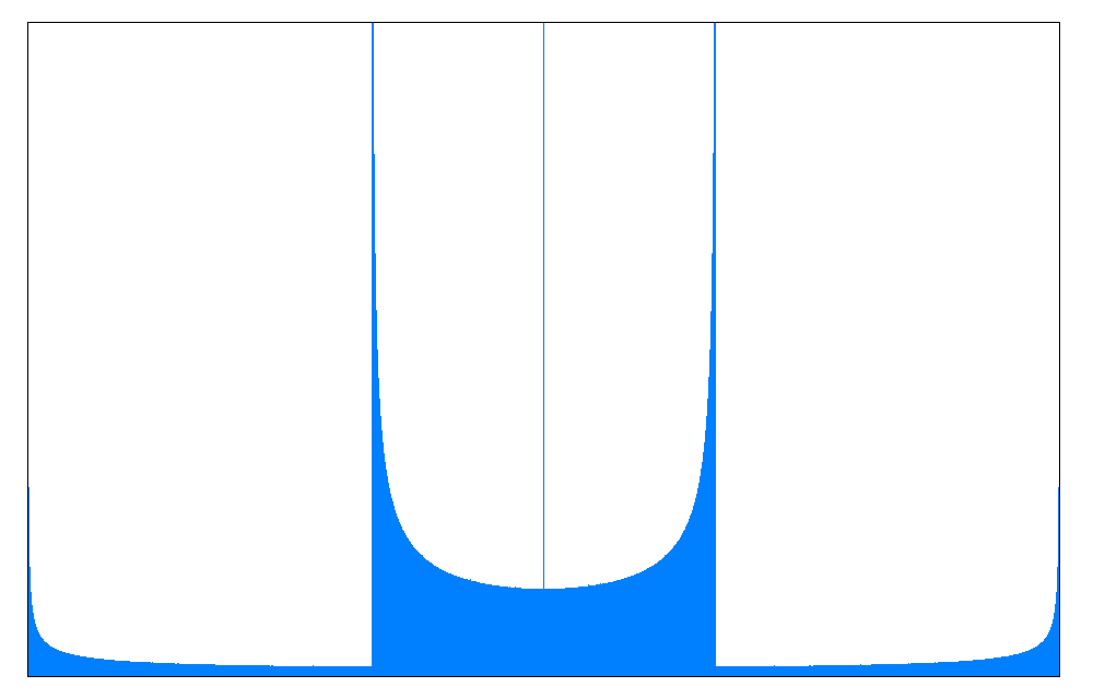
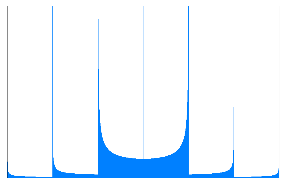
$y^{2}=x^{7}-x$                                      $y^{2}=x^{7}-2x$

Figure 3. $a_{1}$-histograms for two representative curves $C_{2}$.

Based on the data in Table 1, we expect $K_{C_{2}}$ to contain $\mathbb{Q}(i,\sqrt{3},\sqrt[3]{c})$. We now require $c$ to be a cube and restrict to primes $p\equiv 1\bmod 12$ in order to investigate the Sato-Tate distribution of $C_{2}$ over the number field $\mathbb{Q}(i,\sqrt{3},\sqrt[3]{c})$. For $c=1$ we obtain the moments listed below:

$c$	$M_{2}$	$M_{4}$	$M_{6}$	$M_{8}$	$M_{10}$
$1$	10.000	245.997	7299.909	229666.846	7440189.620

The corresponding histogram is shown in Figure 4, and is clearly not the distribution of the identity component; one can see directly that there are (at least) two components.

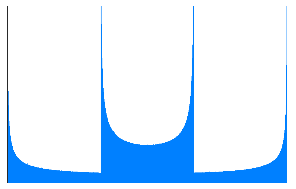
Figure 4. $a_{1}$-histogram for $y^{2}=x^{7}-x$ over $\mathbb{Q}(i,\sqrt{3})$.

This suggests that we should try computing the Sato-Tate distribution over a quadratic extension of $\mathbb{Q}(i,\sqrt{3})$. After a bit of experimentation, one finds that $\mathbb{Q}(i,\sqrt[4]{-3})$ works. With $c=1$ we obtain the moments statistics:

$c$	$M_{2}$	$M_{4}$	$M_{6}$	$M_{8}$	$M_{10}$
$1$	18.000	485.994	14579.770	459261.673	14880044.545

The corresponding histogram is shown in Figure 5.

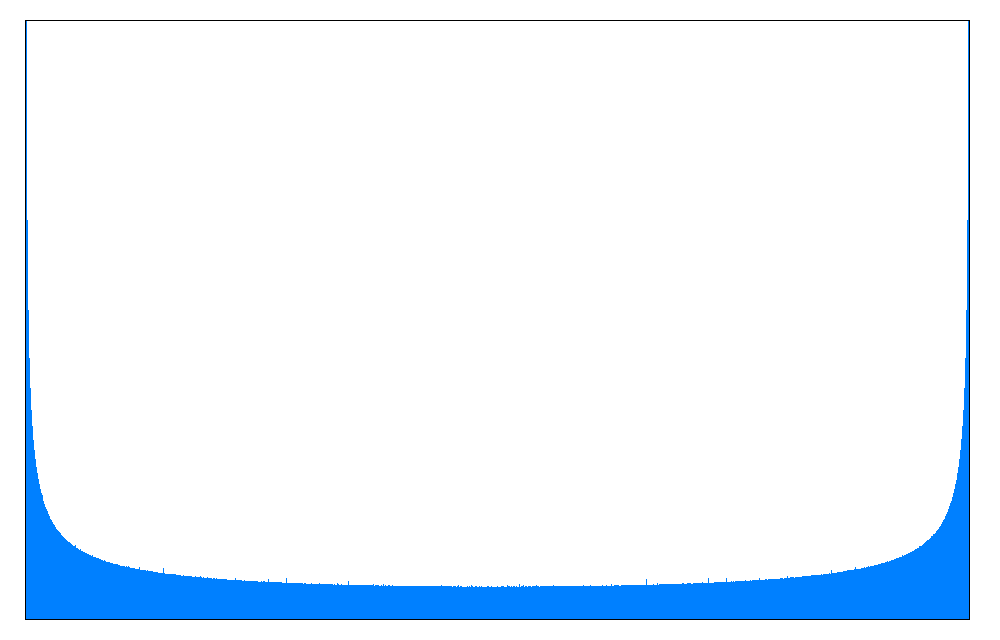
Figure 5. $a_{1}$-histogram for $y^{2}=x^{7}-x$ over $\mathbb{Q}(i,\sqrt[4]{-3})$.

We claim that this distribution corresponds to a connected Sato-Tate group, namely, the group

$${\rm U}(1)_{3}:=\left\langle\begin{bmatrix}U(u)&0&0\\ 0&U(u)&0\\ 0&0&U(u)\end{bmatrix}:u\in{\rm U}(1)\right\rangle.$$

The $a_{1}$-moment sequence for ${\rm U}(1)_{3}$ can be computed as the $3a_{1}$-moment sequence for ${\rm U}(1)$, which simply scales the $n$th moment by $3^{n}$. This yields the moments:

	$M_{2}$	$M_{4}$	$M_{6}$	$M_{8}$	$M_{10}$
${\rm U}(1)_{3}$	18	486	14580	459270	14880348

which are in close agreement (better than 0.1%) with the moment statistics for $y^{2}=x^{7}-x$ over the field $\mathbb{Q}(i,\sqrt[4]{-3})$.

A complication arises if we repeat the experiment using a cube $c\neq 1$; we no longer get a connected Sato-Tate group! Taking $c$ to be a sixth-power works, but we now need to ask whether, generically, the degree 48 extension $\mathbb{Q}(i,\sqrt[4]{-3},\sqrt[6]{c})$ is the minimal extension required to get a connected Sato-Tate group. We have good reason to believe that a degree 24 extension is necessary, since $K_{C_{2}}$ appears to properly contain the degree 12 field $\mathbb{Q}(i,\sqrt{3},\sqrt[3]{c})$, but it is not clear that a degree 48 extension is required. We thus check various quadratic subextensions of $\mathbb{Q}(i,\sqrt[4]{-3},\sqrt[6]{c})$ and find that $\mathbb{Q}(i,\sqrt[3]{c},\sqrt{c\sqrt{-3}})$ works consistently.

We thus conjecture that

$$K_{C_{2}}=\mathbb{Q}(i,\sqrt[3]{c},\sqrt{c\sqrt{-3}}).$$

This implies that for generic $c$, the component group of $\operatorname{ST}(C_{2})$ is isomorphic to

$${\rm Gal}(K_{C_{2}}/\mathbb{Q})\simeq\rm C_{3}\rtimes\rm D_{4}\qquad(\text{GAP id}:\langle 24,8\rangle).$$

As noted above, we conjecture that the identity component is

$$\operatorname{ST}^{0}(C_{2})={\rm U}(1)_{3},$$

up to conjugacy in ${\rm USp}(6)$.

Remark 4.1.

While we are able to give a general description of the Sato-Tate group in both cases just by looking at the $a_{1}$-distribution of the curves $C_{i}$, it should be noted that our characterization of the Sato-Tate group in terms of its identity component and the isomorphism type of its component group is far from sufficient to determine the Sato-Tate distribution. For this we need an explicit description of the Sato-Tate group as a subgroup (up to conjugacy) of ${\rm USp}(6)$; this is addressed in the next section.

5. Determining Sato-Tate groups

In this section we compute the Sato-Tate groups of the curves $C_{1}\colon y^{2}=x^{8}+c$ and $C_{2}\colon y^{2}=x^{7}-cx$ for generic values of $c\in\mathbb{Q}^{*}$. The meaning of generic will be specified in each case, but it ensures that the order of the group of components of the Sato-Tate group is as large as possible. The Sato-Tate groups for the non-generic cases can then be obtained as subgroups.

The description of the Sato-Tate group in terms of the twisted Lefschetz group introduced by Banaszak and Kedlaya [BK15, BK16] is a useful tool for explicitly determining Sato-Tate groups (see [FGL16], for example, where this is exploited), but here we take a different approach that is better suited to our special situation. Our strategy is to identify an elliptic quotient of each of the curves $C_{1}$ and $C_{2}$ and then use the classification results of [FKRS12] to identify the Sato-Tate group of the complement abelian surface. We then reconstruct the Sato-Tate group of the curves $C_{1}$ and  $C_{2}$ from this data.

To determine the splitting of the Jacobians of $C_{1}$ and $C_{2}$ we benefit from the fact that these are curves with large automorphism groups. For generic $c$, the automorphism group of $C_{1}$ over $K_{C_{1}}$ has order 32 (GAP id $\langle 32,9\rangle$), and the automorphism group of $C_{2}$ over $K_{C_{2}}$ has order 24 (GAP id $\langle 24,5\rangle$).

We start by fixing the following matrix notations:

$$I:=\begin{bmatrix}1&0\\ 0&1\end{bmatrix},\,J:=\begin{bmatrix}0&1\\ -1&0\end{bmatrix},\,K:=\begin{bmatrix}0&i\\ i&0\end{bmatrix},\,Z_{n}:=\begin{bmatrix}e^{2\pi i/n}&0\\ 0&e^{-2\pi i/n}\end{bmatrix}.$$

Also, for $u\in{\rm U}(1)$, recall the notation $U(u)$ introduced in (4). Whenever we consider matrices of the unitary symplectic group ${\rm USp}(6)$, we do it with respect to the symplectic form given by the matrix

(6) $$H:=\begin{bmatrix}J&0&0\\ 0&J&0\\ 0&0&J\end{bmatrix}\,.$$

If $A$ and $A^{\prime}$ are two abelian varieties defined over $k$, we write $A\sim A^{\prime}$ to indicate that $A$ and $A^{\prime}$ are related by an isogeny defined over $k$. Finally, we let $\zeta_{3}$ denote a primitive third root of unity in $\overline{\mathbb{Q}}$.

5.1. Sato-Tate group of $C_{1}\colon y^{2}=x^{8}+c$

Lemma 5.1.

Let $c\in\mathbb{Q}^{*}$ and $C_{1}\colon y^{2}=x^{8}+c$. Then

$$\operatorname{Jac}(C_{1})\sim E\times\operatorname{Jac}(C)\,,$$

where $E\colon y^{2}=x^{4}+c$ and $C\colon y^{2}=x^{5}+cx$ over $\mathbb{Q}$. Thus $K_{C_{1}}=\mathbb{Q}(i,\sqrt{-2},c^{1/4})$.

Proof.

First note that we can write nonconstant morphisms defined over $\mathbb{Q}$:

(7) $$\begin{array}[]{l}\phi_{E}:C_{1}\rightarrow E\,,\qquad\phi_{E}(x,y)=(x^{2},y)\,,\\[6.0pt] \phi_{C}:C_{1}\rightarrow C\,,\qquad\phi_{C}(x,y)=(x^{2},xy)\,.\end{array}$$

We clearly have that $K_{E}=\mathbb{Q}(i)$. To see that $K_{C}=\mathbb{Q}(i,\sqrt{-2},c^{1/4})$, first set $F=\mathbb{Q}(c^{1/4})$, and consider the automorphism

$$\alpha\colon C_{F}\rightarrow C_{F},\qquad\alpha(x,y)=\left(\frac{c^{1/2}}{x},\frac{c^{3/4}}{x^{3}}\,y\right).$$

Since $\alpha$ has order $2$ and is nonhyperelliptic, $C_{F}/\langle\alpha\rangle$ is an elliptic curve $E^{\prime}$ defined over $F$. Poincaré’s decomposition theorem implies that $\operatorname{Jac}(C)_{F}\sim E^{\prime}\times E^{\prime\prime}$, where $E^{\prime\prime}$ is an elliptic curve defined over $F$. Observe that we also have the automorphism

$$\gamma\colon C_{F(i)}\rightarrow C_{F(i)},\qquad\gamma(x,y)=(-x,iy)\,.$$

Since $\alpha$ and $\gamma$ do not commute, we deduce that ${\rm End}(\operatorname{Jac}(C)_{F(i)})$ is nonabelian. It follows that $E^{\prime}_{F(i)}$ and $E^{\prime\prime}_{F(i)}$ are $F(i)$-isogenous and that $\operatorname{Jac}(C)_{F(i)}\sim E^{\prime 2}_{F(i)}$. One may readily find an equation for the quotient curve $E^{\prime}=C_{F}/\langle\alpha\rangle$, and, by computing its $j$-invariant, determine that $E^{\prime}$ has complex multiplication by $\mathbb{Q}(\sqrt{-2})$. From this we may conclude that $K_{C}=F(i,\sqrt{-2})$. The asserted splitting of the Jacobian $\operatorname{Jac}(C_{1})$ follows from the existence of the morphisms of equation (7) and the fact that $E$ and $E^{\prime}$ are not $\overline{\mathbb{Q}}$-isogenous. This latter fact also implies that $K_{C_{1}}$ is the compositum of $K_{E}$ and $K_{C}$. ∎

Definition 5.2.

In this subsection, we say that $c\in\mathbb{Q}^{*}$ is generic if $[K_{C_{1}}:\mathbb{Q}]$ is maximal, that is, $[K_{C_{1}}:\mathbb{Q}]=16$. Equivalently, $c\not\in\mathbb{Q}(i,\sqrt{-2})^{*2}$.

Corollary 5.3.

For generic $c\in\mathbb{Q}^{*}$, the Sato-Tate group of $\operatorname{Jac}(C_{1})$ is

$$\left\langle\begin{bmatrix}J&0&0\\ 0&J&0\\ 0&0&J\\ \end{bmatrix},\,\begin{bmatrix}0&J&0\\ -J&0&0\\ 0&0&I\\ \end{bmatrix},\,\begin{bmatrix}Z_{8}&0&0\\ 0&\overline{Z}_{8}&0\\ 0&0&I\\ \end{bmatrix},\,\begin{bmatrix}U(u)&0&0\\ 0&U(u)&0\\ 0&0&U(v)\\ \end{bmatrix}:\,u,v\in{\rm U}(1)\right\rangle\,.$$

Proof.

Recall the notations of Lemma 5.1. It follows from the description of $\operatorname{Jac}(C)$ given in the proof of the lemma and the results of [FKRS12] that $\operatorname{ST}(C)$ can be presented as

$$\left\langle R:=\begin{bmatrix}J&0\\ 0&J\\ \end{bmatrix},\,S:=\begin{bmatrix}0&J\\ -J&0\\ \end{bmatrix},\,T:=\begin{bmatrix}Z_{8}&0\\ 0&\overline{Z}_{8}\\ \end{bmatrix},\,\begin{bmatrix}U(u)&0\\ 0&U(u)\\ \end{bmatrix}:\,u\in{\rm U}(1)\right\rangle\,.$$

This is the group named $J(D_{4})$ in [FKRS12]. Since $E/\mathbb{Q}$ has CM, we also have

$$\operatorname{ST}(E)=\left\langle J,\,U(u):u\in{\rm U}(1)\right\rangle\,.$$

Since $E$ is not a $\overline{\mathbb{Q}}$-isogeny factor of $\operatorname{Jac}(C)$, we have $\operatorname{ST}^{0}(C_{1})\simeq\operatorname{ST}^{0}(E)\oplus\operatorname{ST}^{0}(C)$, which proves the part of the corollary concerning the identity component. By Proposition 2.3, we have isomorphisms

(8) $$\begin{array}[]{l}\psi_{E}\colon\operatorname{ST}(E)/\operatorname{ST}^{0}(E)\overset{\sim}{\longrightarrow}{\rm Gal}(K_{E}/\mathbb{Q})\,,\\[6.0pt] \psi_{C}\colon\operatorname{ST}(C)/\operatorname{ST}^{0}(C)\overset{\sim}{\longrightarrow}{\rm Gal}(K_{C}/\mathbb{Q})\,,\\[6.0pt] \psi_{C_{1}}\colon\operatorname{ST}(C_{1})/\operatorname{ST}^{0}(C_{1})\overset{\sim}{\longrightarrow}{\rm Gal}(K_{C_{1}}/\mathbb{Q})\,.\end{array}$$

The isomorphism $\psi_{E}$ identifies $J$ with the nontrivial automorphism of $K_{E}$, whereas the isomorphism $\psi_{C}$ identifies the images of the generators $g=R,S,T$ in

$$\operatorname{ST}(C)/\operatorname{ST}^{0}(C)\simeq\langle R,S,T\rangle/\langle-1\rangle$$

with automorphisms $\sigma=r,s,t\in{\rm Gal}(K_{C_{1}}/\mathbb{Q})={\rm Gal}(K_{C}/\mathbb{Q})$ as indicated below:

$g$	$\sigma=\psi_{C}(g)$	$\sigma(i)$	$\sigma(\sqrt{-2})$	$\sigma(c^{1/4})$
$R$	$r$	$-i$	$\sqrt{-2}$	$c^{1/4}$
$S$	$s$	$i$	$-\sqrt{-2}$	$c^{1/4}$
$T$	$t$	$i$	$\sqrt{-2}$	$ic^{1/4}$

Let $\mathpzc R,\mathpzc S,\mathpzc T$ be the three first generators of $\operatorname{ST}(C_{1})$. To check the part of the theorem concerning the group of components of $\operatorname{ST}(C_{1})$, one only needs to verify that $\mathpzc R,\mathpzc S,\mathpzc T$ generate a group of components isomorphic to

$${\rm Gal}(K_{C_{1}}/\mathbb{Q})\simeq\langle\mathcal{R},\,\mathcal{S},\,\mathcal{T}\,|\,\mathcal{R}^{2},\,\mathcal{S}^{2},\,\mathcal{T}^{4},\,\mathcal{RSRS},\,\mathcal{RTRT},\,\mathcal{STS}\mathcal{T}^{3}\,\rangle,$$

and that their natural projections onto $\operatorname{ST}(E)/\operatorname{ST}^{0}(E)$ and onto $\operatorname{ST}(C)/\operatorname{ST}^{0}(C)$ are compatible with the isomorphisms of (8). In this case, this amounts to noting that $\mathpzc R,\mathpzc S,\mathpzc T$ project onto $R,S,T$ in $\operatorname{ST}(C)$; that the automorphism $r$ restricts to the non-trivial element of ${\rm Gal}(K_{E}/\mathbb{Q})$, while $\mathpzc R$ projects down to $J$ in $\operatorname{ST}(E)$; and that the restrictions of $s$ and $t$ to $K_{E}$ are trivial, as are the projections of $\mathpzc S$ and $\mathpzc T$ to $\operatorname{ST}(E)$. ∎

Remark 5.4.

We note that even though $\operatorname{Jac}(C_{1})\sim E\times\operatorname{Jac}(C)$, in the generic case the Sato-Tate group $\operatorname{ST}(C_{1})$ is not isomorphic to the direct sum of $\operatorname{ST}(E)$ and $\operatorname{ST}(C)$, because ${\rm Gal}(K_{C_{1}}/\mathbb{Q})$ is not isomorphic to the direct product of ${\rm Gal}(K_{E}/\mathbb{Q})$ and ${\rm Gal}(K_{C}/\mathbb{Q})$. This highlights the importance of being able to write down an explicit description for $\operatorname{ST}(C_{1})$ in terms of generators.

Remark 5.5.

To treat non-generic values of $c$, one replaces $Z_{8}$ in the third generator for $\operatorname{ST}(C_{1})$ in Corollary 5.3 with $Z_{4}$ or $Z_{2}$ when $c\in\mathbb{Q}(i,\sqrt{2})^{*2}\setminus\mathbb{Q}(i,\sqrt{2})^{*4}$ or $c\in\mathbb{Q}(i,\sqrt{2})^{*4}$, respectively (in the latter case one can simply remove $\mathpzc T$ since it is already realized by $u=-1$ and $v=1$).

Using the explicit representation of $\operatorname{ST}(C_{1})$ given in Corollary 5.3 one may compute moment sequences using the techniques described in §3.2 of [FKS13]. The table below lists moments not only for $a_{1}$, but also for $a_{2}$ and $a_{3}$, where $a_{i}$ denotes the coefficient of $T^{i}$ in the characteristic polynomial of a random element of $\operatorname{ST}(C_{1})$ distributed according to the Haar measure (these correspond to normalized $L$-polynomial coefficients of $\operatorname{Jac}(C_{1})$):

	$M_{1}$	$M_{2}$	$M_{3}$	$M_{4}$	$M_{5}$	$M_{6}$	$M_{7}$	$M_{8}$
$a_{1}\colon$	0	2	0	24	0	470	0	11235
$a_{2}\colon$	2	9	56	492	5172	59691	726945	9178434
$a_{3}\colon$	0	9	0	1245	0	284880	0	79208745

The $a_{1}$ moments closely match the corresponding moment statistics listed in Table 1 in the cases where $c$ is generic, as expected. For a further comparison, we computed moment statistics for $a_{1},a_{2}$ $a_{3}$ by applying the algorithm of [HS14b] to the curve $y^{2}=x^{8}+3$ over primes $p\leq 2^{30}$. The $a_{1}$-moment statistics listed below have less resolution than those in Table 1, which covers $p\leq 2^{40}$ (with this higher bound we get $M_{8}\approx 11234$, an even better match to the value $11235$ predicted by the Sato-Tate group $\operatorname{ST}(C_{1})$).

	$M_{1}$	$M_{2}$	$M_{3}$	$M_{4}$	$M_{5}$	$M_{6}$	$M_{7}$	$M_{8}$
$a_{1}\colon$	0.00	2.00	0.00	23.98	0.04	469.26	1	11210
$a_{2}\colon$	2.00	9.00	55.95	491.22	5160.77	59527.55	724556	9143413
$a_{3}\colon$	0.00	8.99	0.04	1242.59	10.30	283980.23	2972	78866094

5.2. Sato-Tate group of $C_{2}\colon y^{2}=x^{7}-cx$

Lemma 5.6.

Let $c\in\mathbb{Q}^{*}$ and $C_{2}\colon y^{2}=x^{7}-cx$. Set $F:=\mathbb{Q}(\zeta_{3},c^{1/3})$. Then

$$\operatorname{Jac}(C_{2})\sim E\times A\,,$$

where $E\colon y^{2}=x^{3}-cx$ and $A$ is an abelian surface defined over $\mathbb{Q}$ for which $A_{F}\sim E^{\prime}\times E^{\prime\prime}$, where $E^{\prime}$ and $E^{\prime\prime}$ are elliptic curves defined over $F$ by the equations

$$E^{\prime}\colon y^{2}=x^{3}+3c^{1/3}x\,,\qquad E^{\prime\prime}\colon y^{2}=x^{3}+3\zeta_{3}c^{1/3}x\,.$$

Thus $K_{C_{2}}=\mathbb{Q}(i,c^{1/3},\sqrt{c\sqrt{-3}})$.

Proof.

We can write nonconstant morphisms:

$$\begin{array}[]{l}\phi_{E}\colon(C_{2})_{F}\rightarrow E_{F}\,,\qquad\qquad\hskip 3.0pt\phi_{E}(x,y)=(x^{3},xy)\,,\\[6.0pt] \phi_{E^{\prime}}\colon(C_{2})_{F}\rightarrow E^{\prime}\,,\qquad\qquad\hskip 4.0pt\phi_{E^{\prime}}(x,y)=\left(\frac{x^{2}-c^{1/3}}{x},\frac{y}{x^{2}}\right),\\[6.0pt] \phi_{E^{\prime\prime}}\colon(C_{2})_{F}\rightarrow E^{\prime\prime}\,,\qquad\qquad\phi_{E^{\prime\prime}}(x,y)=\left(\frac{x^{2}-\zeta_{3}c^{1/3}}{x},\frac{y}{x^{2}}\right).\end{array}$$

Note that the morphisms $\phi_{E}$, $\phi_{E^{\prime}}$, and $\phi_{E^{\prime\prime}}$ are quotient maps given by automorphisms $\alpha_{E}$, $\alpha_{E^{\prime}}$, and $\alpha_{E^{\prime\prime}}$ of $(C_{2})_{F}$:

$$\alpha_{E}(x,y):=(\zeta_{3}x,\zeta_{3}^{2}y)\,,\quad\alpha_{E^{\prime}}(x,y):=\left(\frac{-c^{1/3}}{x},\frac{c^{2/3}y}{x^{4}}\right)\,,\quad\alpha_{E^{\prime\prime}}:=\alpha_{E}\circ\alpha_{E^{\prime}}\,.$$

To see that $\operatorname{Jac}(C_{2})_{F}\sim E_{F}\times E^{\prime}\times E^{\prime\prime}$, it is enough to check that we have an isomorphism of $F$-vector spaces of regular differential forms

$$\Omega_{(C_{2})_{F}}=\phi_{E}^{*}(\Omega_{E_{F}})\oplus\phi_{E^{\prime}}^{*}(\Omega_{E^{\prime}})\oplus\phi_{E^{\prime\prime}}^{*}(\Omega_{E^{\prime\prime}})\,,$$

But this follows from the fact that $\omega_{1}=dx/y$, $\omega_{2}=x\cdot dx/y$, and $\omega_{3}=x^{2}\cdot dx/y$ constitute a basis for $\Omega_{(C_{2})_{F}}$, together with the easy computation

$$\phi_{E}^{*}\left(\frac{dx}{y}\right)=3\omega_{2},\quad\phi_{E^{\prime}}^{*}\left(\frac{dx}{y}\right)=c^{1/3}\omega_{1}+\omega_{3},\quad\phi_{E^{\prime\prime}}^{*}\left(\frac{dx}{y}\right)=\zeta_{3}c^{1/3}\omega_{1}+\omega_{3}.$$

Since $E$ is defined over $\mathbb{Q}$, there exists an abelian surface $A$ defined over $\mathbb{Q}$ such that $A_{F}\sim E^{\prime}\times E^{\prime\prime}$. To see that $K_{C_{2}}=\mathbb{Q}(i,c^{1/3},\sqrt{c\sqrt{-3}})$, first note that $F(i)\subseteq K_{C_{2}}$ and that $E^{\prime}\sim E^{\prime\prime}$. Therefore, $K_{C_{2}}$ is the minimal extension of $F(i)$ over which $E$ and $E^{\prime}$ become isomorphic. Now observe that we have an isomorphism

(9) $$\psi\colon E_{F(i,\sqrt{c\sqrt{-3}})}\rightarrow E^{\prime}_{F(i,\sqrt{c\sqrt{-3}})}\,,\qquad\psi(x,y)=\left(\frac{\sqrt{-3}}{c^{1/3}}x,\frac{\sqrt{-3}\sqrt{c\sqrt{-3}}}{c}y\right),$$

from which we see that $K_{C_{2}}$ is the extension of $F(i)$ obtained by adjoining the element $\sqrt{c\sqrt{-3}}$ to $F(i)$ (note: one needs to write formula in (9) carefully, otherwise one may be tempted to make $K_{C_{2}}$ too large). ∎

Definition 5.7.

In this subsection, we say that $c\in\mathbb{Q}^{*}$ is generic if $[K_{C_{2}}:\mathbb{Q}]$ is maximal, that is, $[K_{C_{2}}:\mathbb{Q}]=24$. Equivalently, $c$ is not a cube in $\mathbb{Q}^{*}$.

Corollary 5.8.

For generic $c\in\mathbb{Q}^{*}$, the Sato-Tate group of $\operatorname{Jac}(C_{2})$ is

$$\left\langle\begin{bmatrix}J&0&0\\ 0&J&0\\ 0&0&J\\ \end{bmatrix},\,\begin{bmatrix}0&K&0\\ K&0&0\\ 0&0&J\\ \end{bmatrix},\,\begin{bmatrix}Z_{3}&0&0\\ 0&\overline{Z}_{3}&0\\ 0&0&I\\ \end{bmatrix},\,\begin{bmatrix}U(u)&0&0\\ 0&U(u)&0\\ 0&0&U(u)\\ \end{bmatrix}:\,u\in{\rm U}(1)\right\rangle\,.$$

Proof.

We assume the notations of Lemma 5.6. Since $E$, $E^{\prime}$, and $E^{\prime\prime}$ are $K_{C_{2}}$-isogenous, we have $\operatorname{ST}^{0}(C_{2})\simeq{\rm U}(1)$. Note that $K_{A}=\mathbb{Q}(i,\zeta_{3},c^{1/3})$. We claim that $\operatorname{ST}(A)$ is the group named $D_{6,1}$ in [FKRS12]. As may be seen in [FKRS12, Table 8], there are three Sato-Tate groups with identity component ${\rm U}(1)$ and group of components isomorphic to ${\rm Gal}(K_{A}/\mathbb{Q})\simeq D_{6}$, namely, $J(D_{3})$, $D_{6,1}$, and $D_{6,2}$. We can rule out the latter option, since by [FKRS12, Table 2] this would imply that ${\rm Gal}(K_{A}/\mathbb{Q}(i))$ is a cyclic group of order $6$, which is false. To rule out $J(D_{3})$, we need to argue along the lines of [FKRS12, §4.6]: Let $F$ denote $\mathbb{Q}(\zeta_{3},c^{1/3})$ as in Lemma 5.6; if $\operatorname{ST}(A)=J(D_{3})$, then $\operatorname{ST}(A_{F})=J(C_{1})$, whereas if $\operatorname{ST}(A)=D_{6,1}$, then $\operatorname{ST}(A_{F})=C_{2,1}$. By the dictionary between Sato-Tate groups and Galois endomorphism types in dimension $2$ given by Theorem 2.5 (see [FKRS12, Table 8]), the first option would imply that ${\rm End}(A_{F})\otimes_{\mathbb{Z}}\mathbb{R}$ is isomorphic to the Hamilton quaternion algebra $\mathbb{H}$, whereas the second option would yield ${\rm End}(A_{F})\otimes_{\mathbb{Z}}\mathbb{R}\simeq\mathrm{M}_{2}(\mathbb{R})$. Since Lemma 5.6, ensures that we are in the latter case, we must have $\operatorname{ST}(A)=D_{6,1}$.

For convenience, we take the following presentation of $D_{6,1}$, which is conjugate to the one given in [FKRS12]:

$$\left\langle R:=\begin{bmatrix}J&0\\ 0&J\\ \end{bmatrix},\,S:=\begin{bmatrix}0&K\\ K&0\\ \end{bmatrix},\,T:=\begin{bmatrix}Z_{3}&0\\ 0&\overline{Z}_{3}\\ \end{bmatrix},\,\begin{bmatrix}U(u)&0\\ 0&U(u)\\ \end{bmatrix}:u\in{\rm U}(1)\right\rangle\,.$$

Since $E/\mathbb{Q}$ has CM, we have

$$\operatorname{ST}(E)=\left\langle J,\,U(u):u\in{\rm U}(1)\right\rangle\,.$$

By Proposition 2.3, we have isomorphisms

$$\begin{array}[]{l}\psi_{E}\colon\operatorname{ST}(E)/\operatorname{ST}^{0}(E)\overset{\sim}{\longrightarrow}{\rm Gal}(K_{E}/\mathbb{Q})\,,\\[6.0pt] \psi_{A}\colon\operatorname{ST}(A)/\operatorname{ST}^{0}(A)\overset{\sim}{\longrightarrow}{\rm Gal}(K_{A}/\mathbb{Q})\,,\\[6.0pt] \psi_{C_{2}}\colon\operatorname{ST}(C_{2})/\operatorname{ST}^{0}(C_{2})\overset{\sim}{\longrightarrow}{\rm Gal}(K_{C_{2}}/\mathbb{Q})\,.\end{array}$$

To prove the corollary it suffices to make these isomorphisms explicit and show that they are compatible with the projections from $\operatorname{ST}(C_{2})$ to $\operatorname{ST}(E)$ and $\operatorname{ST}(A)$, and with the restriction maps from ${\rm Gal}(K_{C_{2}}/\mathbb{Q})$ to ${\rm Gal}(K_{E}/\mathbb{Q})$ and ${\rm Gal}(K_{A}/\mathbb{Q})$.

The isomorphism $\psi_{E}$ identifies the image of $J$ in $\operatorname{ST}(E)/\operatorname{ST}^{0}(E)$ with the non-trivial element of ${\rm Gal}(K_{E}/\mathbb{Q})$, while the isomorphism $\psi_{A}$ identifies the images of the generators $g=R,S,T$ in

$$\operatorname{ST}(A)/\operatorname{ST}^{0}(A)\simeq\langle R,S,T\rangle/\langle-1\rangle$$

with automorphisms $\sigma=r,s,t\in{\rm Gal}(K_{A}/\mathbb{Q})$ as indicated below:

$g$	$\sigma=\psi_{A}(g)$	$\sigma(i)$	$\sigma(\zeta_{3})$	$\sigma(c^{1/3})$
$R$	$r$	$-i$	$\zeta_{3}^{2}$	$c^{1/3}$
$S$	$s$	$-i$	$\zeta_{3}$	$c^{1/3}$
$T$	$t$	$i$	$\zeta_{3}$	$\zeta_{3}c^{1/3}$

If we now let $\mathpzc R,\mathpzc S,\mathpzc T$ denote the first three generators of $\operatorname{ST}(C_{2})$ listed in the corollary, $\psi_{C_{2}}$ identifies their images in $\operatorname{ST}(C_{2})/\operatorname{ST}^{0}(C_{2})$ with elements of ${\rm Gal}(K_{A}/\mathbb{Q})$ as indicated below, where $\delta=\sqrt{c\sqrt{-3}}$:

$g$	$\sigma=\psi_{C_{2}}(g)$	$\sigma(i)$	$\sigma(\zeta_{3})$	$\sigma(c^{1/3})$	$\sigma(\delta)$
$\mathpzc R$	$\mathpzc r$	$-i$	$\zeta_{3}^{2}$	$c^{1/3}$	$i\delta$
$\mathpzc S$	$\mathpzc s$	$-i$	$\zeta_{3}$	$c^{1/3}$	$\delta$
$\mathpzc T$	$\mathpzc t$	$i$	$\zeta_{3}$	$\zeta_{3}\,c^{1/3}$	$\delta$

We note that, unlike their restrictions $r$ and $s$, the automorphisms $\mathpzc r$ and $\mathpzc s$ do not commute, they generate a dihedral group of order $8$ inside ${\rm Gal}(K_{C_{2}}/\mathbb{Q})$. The three automorphisms $\mathpzc r,\mathpzc s,\mathpzc t$ together generate ${\rm Gal}(K_{C_{2}}/\mathbb{Q})$. Their restrictions to $K_{A}$ are the generators $r,s,t$ for $K_{A}$, and $R,S,T$ are the projections of $\mathpzc R,\mathpzc S,\mathpzc T$ to $\operatorname{ST}(A)$. The automorphisms $\mathpzc r$ and $\mathpzc s$ both restrict to the non-trivial element of ${\rm Gal}(K_{E}/\mathbb{Q})$, and both $\mathpzc R$ and $\mathpzc S$ project down to $J$ in $\operatorname{ST}(E)$. The restriction of $\mathpzc t$ to $K_{E}$ is trivial, as is the projection of $\mathpzc T$ to $\operatorname{ST}(E)$. To complete the proof it suffices to verify that the map

$$\operatorname{ST}(C_{2})/\operatorname{ST}^{0}(C_{2})\simeq\langle\mathpzc R,\mathpzc S,\mathpzc T\rangle/\langle-1\rangle\xrightarrow{\quad\psi_{C_{2}}\quad}\langle\mathpzc r,\mathpzc s,\mathpzc t\rangle\simeq{\rm Gal}(K_{C_{2}}/\mathbb{Q})$$

we have explicitly defined is indeed an isomorphism. One can check that both sides are isomorphic to the finitely presented group

$$\langle\mathcal{R,S,T}\,|\,\mathcal{R}^{2},\mathcal{S}^{2},\mathcal{T}^{3},\mathcal{RSRSRSRS,RTRT,STST}^{2}\rangle,$$

via maps that send generators to corresponding generators (in the order shown). ∎

Remark 5.9.

To treat non-generic values of $c$, simply remove the third generator containing $Z_{3}$ from the list of generators for $\operatorname{ST}(C_{2})$ in Corollary 5.8 when $c$ is a cube in $\mathbb{Q}^{*}$.

Using the explicit representation of $\operatorname{ST}(C_{2})$ given in Corollary 5.8, one may compute moments sequences for the characteristic polynomial coefficients $a_{1},a_{2},a_{3}$ using the techniques described in §3.2 of [FKS13]; the first eight moments are listed below:

	$M_{1}$	$M_{2}$	$M_{3}$	$M_{4}$	$M_{5}$	$M_{6}$	$M_{7}$	$M_{8}$
$a_{1}\colon$	0	2	0	30	0	720	0	20650
$a_{2}\colon$	2	10	75	784	9607	126378	1721715	23928108
$a_{3}\colon$	0	11	0	2181	0	660790	0	224864661

The $a_{1}$ moments closely match the corresponding moment statistics listed in Table 2 in the cases where $c$ is generic, as expected. We also computed moment statistics for $a_{1},a_{2}$ and $a_{3}$ by applying the algorithm of [HS14b] to the curve $y^{2}=x^{7}-2x$ over primes $p\leq 2^{30}$. The $a_{1}$-moment statistics listed below have less resolution than Table 2, which covers $p\leq 2^{40}$ (with this higher bound we get $M_{8}\approx 20649$, very close to the value $20650$ predicted by $\operatorname{ST}(C_{2})$).

	$M_{1}$	$M_{2}$	$M_{3}$	$M_{4}$	$M_{5}$	$M_{6}$	$M_{7}$	$M_{8}$
$a_{1}\colon$	0.00	2.00	0.00	30.00	0.04	719.62	2	20636
$a_{2}\colon$	2.00	10.00	74.97	783.59	9600.64	126281.75	1720266	23906297
$a_{3}\colon$	0.00	11.00	0.04	2179.67	19.68	660247.53	8549	224645654

6. Galois endomorphism types

As recalled in §2, up to dimension 3, the Galois endomorphism type of an abelian variety over a number field is determined by its Sato-Tate group. In this section, we derive the Galois endomorphism type of $\operatorname{Jac}(C_{2})$ from $\operatorname{ST}(C_{2})$ for generic values of $c$ (in the sense of §5.2). The case of $\operatorname{Jac}(C_{1})$, although leading to slightly larger diagrams, is completely analogous.

Let $G:=\operatorname{ST}(C_{2})$ and $V:={\rm End}(\operatorname{Jac}(C_{2})_{K_{C_{2}}})$, and set $V_{\mathbb{C}}:=V\otimes_{\mathbb{Z}}\mathbb{C}$ and $V_{\mathbb{R}}:=V\otimes_{\mathbb{Z}}\mathbb{R}$. As described in the proof of [FKRS12, Prop. 2.19]:

• $V_{\mathbb{C}}$ is the subspace of $\mathrm{M}_{6}(\mathbb{C})$ fixed by the action of $G^{0}$;

• $V_{\mathbb{R}}$ is the subspace of $V_{\mathbb{C}}$, of half the dimension, over which the Rosati form is positive definite;

• If $L/\mathbb{Q}$ is a subextension of $K_{C_{2}}/\mathbb{Q}$, corresponding to the subgroup $N\subseteq{\rm Gal}(K_{C_{2}}/\mathbb{Q})\simeq G/G^{0}$, then ${\rm End}(\operatorname{Jac}(C_{2})_{L})\otimes_{\mathbb{Z}}\mathbb{R}\simeq V_{\mathbb{R}}^{N}$.

The matrices $\Phi\in\mathrm{M}_{6}(\mathbb{C})$ commuting with $G^{0}\simeq{\rm U}(1)$, embedded in ${\rm USp}(6)$, are matrices of the form $\Phi=(\phi_{i,j})$ with $i,j\in[1,6]$ such that $\phi_{i,j}\in\mathbb{C}$ is $0$ unless $i\equiv j\mod 2$. The condition of the Rosati form being positive definite on $V_{\mathbb{R}}$ amounts to requiring that

$$\operatorname{Trace}(\Phi H^{t}\Phi^{t}H)\geq 0$$

for every $\Phi\in V_{\mathbb{R}}$, where $H$ is the symplectic matrix given in (6). Imposing the above condition on $\Phi$, we find that

$$\Phi=\begin{pmatrix}\alpha&0&\beta&0&\gamma&0\\ 0&\overline{\alpha}&0&\overline{\beta}&0&\overline{\gamma}\\ \delta&0&\epsilon&0&\phi&0\\ 0&\overline{\delta}&0&\overline{\epsilon}&0&\overline{\phi}\\ \lambda&0&\mu&0&\nu&0\\ 0&\overline{\lambda}&0&\overline{\mu}&0&\overline{\nu}\\ \end{pmatrix}\qquad\text{with }\alpha,\beta,\dots,\mu,\nu\in\mathbb{C}\,.$$

We thus deduce that $V_{\mathbb{R}}\simeq\mathrm{M}_{3}(\mathbb{C})$.

We now proceed to determine the sub-$\mathbb{R}$-algebras of $V_{\mathbb{R}}$ fixed by each of the subgroups of ${\rm Gal}(K_{C_{2}}/\mathbb{Q})\simeq G/G^{0}$. With notations as in the proof of Corollary 5.8, these subgroups are listed (up to conjugation) in Figure 6, where normal subgroups are marked with a ^∗. We can then reconstruct the Galois type of $\operatorname{Jac}(C_{2})$ (see Figure 7) from the information in Table 3.

Figure 6. Lattice of subgroups of ${\rm Gal}(K_{C_{2}}/\mathbb{Q})$.

$N$	Condition on $\Phi$	$V_{\mathbb{R}}^{N}$
$\langle\mathpzc R\rangle$	$\alpha,\beta,\dots,\mu,\nu\in\mathbb{R}$	$\mathrm{M}_{3}(\mathbb{R})$
$\langle\mathpzc S\rangle$	$\alpha=\overline{\epsilon},\beta=\overline{\delta},\phi=i\overline{\gamma},\mu=-i\overline{\lambda},\nu\in\mathbb{R}$	$\mathrm{M}_{3}(\mathbb{R})$
$\langle\mathpzc T\rangle$	$\beta=\gamma=\delta=\phi=\lambda=\mu=0$	$\mathbb{C}\times\mathbb{C}\times\mathbb{C}$
$\langle(\mathpzc{RS})^{2}\rangle$	$\gamma=\phi=\lambda=\mu=0$	$\mathrm{M}_{2}(\mathbb{C})\times\mathbb{C}$
$\langle(\mathpzc{RS})^{2},\mathpzc S\rangle$	$\gamma=\phi=\lambda=\mu=0,\alpha=\overline{\epsilon},\beta=\overline{\delta},\nu\in\mathbb{R}$	$\mathrm{M}_{2}(\mathbb{R})\times\mathbb{R}$
$\langle\mathpzc{RS}\rangle$	$\gamma=\phi=\lambda=\mu=0,\alpha=\epsilon,\beta=\delta$	$\mathbb{C}\times\mathbb{C}\times\mathbb{C}$

Table 3. Some subgroups of ${\rm Gal}(K_{C_{2}}/\mathbb{Q})$ with the respective fixed sub-$\mathbb{R}$-algebras of $V_{\mathbb{R}}$.

Obtaining the data in Table 3 is a straight-forward exercise, let us make just a few specific comments:

• $N=\langle\mathpzc S\rangle$: One easily checks that the matrices $\Phi$ satisfying the required condition form a simple nondivision $\mathbb{R}$-algebra; by Wedderburn’s structure theorem, it is of the form $\mathrm{M}_{d}(D)$, for some division algebra $D$ and $d>1$; since its real dimension is $9$, we must have $d=3$ and $D=\mathbb{R}$.

• $N=\langle(\mathpzc{RS})^{2},\mathpzc S\rangle$: Note that the $\mathbb{R}$-algebra

  $$\mathpzc H:=\left\{A_{\alpha,\beta}:=\begin{pmatrix}\alpha&\beta\\ \overline{\beta}&\overline{\alpha}\end{pmatrix}:\alpha,\beta\in\mathbb{C}\right\}$$

  is isomorphic to $\mathrm{M}_{2}(\mathbb{R})$. Indeed, if $\alpha=\alpha_{1}+i\alpha_{2}$ and $\beta=\beta_{1}+i\beta_{2}$, then

  $$\psi\colon\mathpzc H\rightarrow\mathrm{M}_{2}(\mathbb{R})\,,\qquad\psi(A_{\alpha,\beta})=\begin{pmatrix}\alpha_{1}+\beta_{1}&-\alpha_{2}+\beta_{2}\\ \alpha_{2}+\beta_{2}&\alpha_{1}-\beta_{1}\end{pmatrix}$$

  provides the required isomorphism. Alternative, one can reach the same conclusion by noting that $\mathpzc H$ is the only non-commutative $\mathbb{R}$-algebra of dimension 4 with zero divisors.

• $N=\langle\mathpzc{RS}\rangle$: Note that the $\mathbb{R}$-algebra

  $$\mathpzc H:=\left\{A_{\alpha,\beta}:=\begin{pmatrix}\alpha&\beta\\ \beta&\alpha\end{pmatrix}:\alpha,\beta\in\mathbb{C}\right\}$$

  is isomorphic to $\mathbb{C}\times\mathbb{C}$ by means of

  $$\psi\colon\mathpzc H\rightarrow\mathrm{\mathbb{C}}\times\mathbb{C}\,,\qquad\psi(A_{\alpha,\beta})=(\alpha+\beta,\alpha-\beta)\,.$$

Figure 7. Galois endomorphism types of $\operatorname{Jac}(C_{2})$. Lattice of fixed sub-$\mathbb{R}$-algebras corresponding to the subgroups of Figure 6.

References

- [Bac90] E. Bach, Explicit bounds for primality testing and related problems, Math. Comp. 55 (1990), 335–380.
- [Bas04] J.M. Basilla, On the solution of , Proc. Japan Acad. Ser. A Math. Sci. 80 (2004), 40–41.
- [BEW98] B. Berndt, R. Evans, K. Williams, Gauss and Jacobi sums, Wiley, 1998.
- [BK15] G. Banaszak and K.S. Kedlaya, An algebraic Sato-Tate group and Sato-Tate conjecture, Indiana Univ. Math. J. 64 (2015), 245–274.
- [BZ10] R.P. Brent and P. Zimmerman, An algorithm for the Jacobi symbol, Algorithmic Number Theory 9th International Symposium (ANTS IX), LNCS 6197, Springer, 2010, 83–95.
- [Coh93] H. Cohen, A course in computational algebraic number theory, Springer, 1993.
- [Erd61] P. Erdös, Remarks on number theory. I, Mat. Lapok 12 (1961) 10–17.
- [FKRS12] F. Fité, K.S. Kedlaya, V. Rotger, and A.V. Sutherland, Sato-Tate distributions and Galois endomorphism modules in genus , Compos. Math. 148 (2012), 1390–1442.
- [FGL16] F. Fité, J. González, J-C. Lario, Frobenius distribution for quotients of Fermat curves of prime exponent, Canad. J. Math, published online 2016-02-05, to appear in print.
- [FKS13] F. Fité, K.S. Kedlaya, and A.V. Sutherland, Sato-Tate groups of some weight motives, arXiv:1212.0256.
- [FKT04] E. Furukawa, M. Kawazoe, and T. Takahashi, Counting points for hyperelliptic curves of type over finite prime fields, in Selected Areas in Cryptography, LNCS 3006, Springer, 2004, 26–41.
- [GG13] J. von zur Gathen and J. Gerhard, Modern computer algebra, 3rd ed., Cambridge University Press, 2013.
- [HS14a] D. Harvey and A.V. Sutherland, Computing Hasse–Witt matrices of hyperelliptic curves in average polynomial time, in Algorithmic Number Theory 11th International Symposium (ANTS XI), LMS J. Comput. Math. (2014), 257-273.
- [HS14b] D. Harvey and A.V. Sutherland, Computing Hasse–Witt matrices of hyperelliptic curves in average polynomial time, II, arXiv:1410.5222.
- [Man61] Yu. I. Manin, The Hasse-Witt matrix of an algebraic curve, AMS Translations, Series 2 45 (1965), 245–264, (originally published in Izv. Akad. Nauk SSSR Ser. Mat. 25 (1961) 153–172).
- [PW03] X. Wang and V. Pan, Acceleration of Euclidean algorithm and rational number reconstruction, SIAM J. Comput. 32 (2003), 548–556.
- [SS71] A. Schönhage and V. Strassen, Schnelle Multiplikation grosser Zahlen, Computing (Arch. Elektron. Rechnen) 7 (1971), 281–292.
- [Sch85] R. Schoof, Elliptic curves over finite fields and the computation of square roots mod , Math. Comp. 44 (1985), 483–494.
- [SS14] I. Shparlinski and A.V. Sutherland, On the distribution of Atkin and Elkies primes for reductions of elliptic curves on average, LMS J. Comput. Math. 15 (2015), 308–322.
- [Ser12] J.-P. Serre, Lectures on , A.K. Peters/CRC Press, 2012.
- [Sil94] J. Silverman, Advanced topics in the arithmetic of elliptic curves, Springer, 1994.
- [Sut11] A.V. Sutherland, Structure computation and discrete logarithms in finite abelian -groups, Math. Comp. 80 (2011), 477-500.
- [Yui78] Noriko Yui, On the Jacobian varieties of hyperelliptic curves over fields of characteristic , J. Algebra 52 (1978), 378–410.