Action-based distribution functions for spheroidal galaxy components

Abstract

We present an approach to the design of distribution functions that depend on the phase-space coordinates through the action integrals. The approach makes it easy to construct a dynamical model of a given stellar component. We illustrate the approach by deriving distribution functions that self-consistently generate several popular stellar systems, including the Hernquist, Jaffe, and Navarro, Frenk and White models. We focus on non-rotating spherical systems, but extension to flattened and rotating systems is trivial. Our distribution functions are easily added to each other and to previously published distribution functions for discs to create self-consistent multi-component galaxies. The models this approach makes possible should prove valuable both for the interpretation of observational data and for exploring the non-equilibrium dynamics of galaxies via N-body simulations.

1 Introduction

Axisymmetric equilibrium models are extremely useful tools for the study of galaxies. A real galaxy will never be in perfect dynamical equilibrium – it might be accreting dwarf satellites, or being tidally disturbed by the gravitational field of the group or cluster to which it belongs, or displaying spiral structure – but an axisymmetric equilibrium model will usually provide a useful basis from which a more realistic model can be constructed by perturbation theory.

By Jeans (1915) theorem, every equilibrium model can be described by a distribution function (DF) that depends on the phase-space coordinates $({\bf x},{\bf v})$ only through isolating integrals of motion. In an axisymmetric potential, most orbits prove to be quasiperiodic, with the consequence that they admit three isolating integrals (Arnold, 1978). Consequently, a generic DF for an axisymmetric equilibrium galaxy is a function of three variables.

The major obstacle to exploiting this insight is that we have analytic expressions for only two isolating integrals of motion in a general axisymmetric potential, namely the energy $E={\textstyle{1\over 2}}v^{2}+\Phi({\bf x})$ and the component of the angular momentum about the symmetry axis, $J_{\phi}=({\bf x}\times{\bf v})_{z}$. Several authors have examined model galaxies with DFs of the two-integral form $f(E,J_{\phi})$ (Prendergast & Tomer, 1970; Wilson, 1975; Rowley, 1988; Evans, 1994), but in such models the velocity dispersions $\sigma_{R}$ and $\sigma_{z}$ in the radial and vertical directions are inevitably equal. This condition is seriously violated in our Galaxy and we have no reason to suppose that the condition is better satisfied in any external galaxy. Hence it is mandatory to extend the DF’s argument list to include a “non-classical” integral, $I_{3}$, for which we do not have a convenient expression.

Since any function $J(E,J_{\phi},I_{3})$ of three isolating integrals is itself an isolating integral, we actually have an enormous amount of freedom as to what integrals to use as arguments of the DF. Given that we must use at least one integral for which we lack an expression for its dependence on $({\bf x},{\bf v})$, there is a powerful case for making the DF’s arguments action integrals. These integrals are alone capable as serving as the three momenta $J_{i}$ of a canonical coordinate system – this property makes them the bedrock of perturbation theory. Their canonically conjugate variables, the angles $\theta_{i}$, have two remarkable properties: (i) along any orbit they increase linearly with time at rates $\Omega_{i}({\bf J})$, so

$$\theta_{i}(t)=\theta_{i}(0)+\Omega_{i}({\bf J})\,t,$$ (1)

and (ii) they make the ordinary phase-space coordinates periodic functions

$${\bf x}({\mathchoice{\hbox{{\gkvecten\char 18\relax}}}{\hbox{{\gkvecten\char 18\relax}}}{\hbox{{\gkvecseven\char 18\relax}}}{\hbox{{\gkvecseven\char 18\relax}}}}+2\pi{\bf m},{\bf J})={\bf x}({\mathchoice{\hbox{{\gkvecten\char 18\relax}}}{\hbox{{\gkvecten\char 18\relax}}}{\hbox{{\gkvecseven\char 18\relax}}}{\hbox{{\gkvecseven\char 18\relax}}}},{\bf J})\quad(\hbox{integer }m_{i}).$$ (2)

The actions $J_{i}$ also have nice properties. In particular, (i) any triple of finite numbers $(J_{r},J_{\phi},J_{z})$ with $J_{r},J_{z}\geq 0$ corresponds to a bound orbit with the orbit ${\bf J}=0$ being that on which a star is stationary at the middle of the galaxy, and (ii) the volume of phase space occupied by orbits with actions in ${\rm d}^{3}{\bf J}$ is $(2\pi)^{3}{\rm d}^{3}{\bf J}$. Consequently, any non-negative function $f({\bf J})$ that tends to zero as $|{\bf J}|\to\infty$ and has a finite integral $\int{\rm d}^{3}{\bf J}\,f({\bf J})$ specifies a valid galaxy model of mass

$$M=(2\pi)^{3}\int{\rm d}^{3}{\bf J}\,f({\bf J}).$$ (3)

The actions are defined by integrals

$$J_{i}={1\over 2\pi}\oint_{\gamma_{i}}{\rm d}{\bf x}\cdot{\bf v},$$ (4)

where $\gamma_{i}$ is a closed path in phase space. If we require that the first action $J_{r}$ quantifies the extent of a star’s radial excursions and the third action $J_{z}$ quantifies the extent of its excursions either side of the potential’s equatorial plane, then the actions are unambiguously defined. What we here call $J_{r}$ is sometimes called $J_{R}$ or $J_{u}$, and what we call $J_{z}$ is sometimes called $J_{\vartheta}$ or $J_{v}$, but no significance attaches to these different notations. In a spherical potential $J_{z}=L-|J_{\phi}|$, where $L$ is the magnitude of the angular momentum vector.

To obtain the observable properties of a model defined by $f({\bf J})$, for example its density distribution $\rho({\bf x})=\int{\rm d}^{3}{\bf v}\,f({\bf J})$ and its velocity dispersion tensor $\sigma^{2}_{ij}({\bf x})$, one has to be able to evaluate ${\bf J}({\bf x},{\bf v})$ in an arbitrary gravitational potential. Recently a number of techniques have been developed for doing this (Binney, 2012a; Sanders & Binney, 2014, 2015). Consequently, while the last word on action evaluation has likely not yet been written, we now have algorithms that enable one to extract the observables from a DF $f({\bf J})$ with reasonable accuracy.

DFs $f({\bf J})$ that depend on the phase-space coordinates only through the actions were first used to model the disc of our Galaxy in an assumed gravitational potential (Binney, 2010, 2012b). Recently Binney (2014, hereafter B14) showed how to derive the self-consistent gravitational potential that is implied by a given $f({\bf J})$ by exploring a family of flattened, rotating models that he derived from the “ergodic” DF of the isochrone model: that is the DF $f(H)$ that depends on the phase-space coordinates only through the Hamiltonian $H=\frac{1}{2}v^{2}+\Phi({\bf x})$. Hénon (1960) derived the isochrone’s ergodic DF, and in the case of the isochrone potential explicit expressions are available for ${\bf J}({\bf x},{\bf v})$ and $H({\bf J})$ (Gerhard & Saha, 1991). Substituting $H({\bf J})$ in $f(H)$ B14 obtained the DF $f({\bf J})$ of the isotropic isochrone model. In this paper we present simple analytic functions $f({\bf J})$ that generate nearly isotropic models of other widely used models, such as the Hernquist (1990), Jaffe (1983), and Navarro, Frenk, & White (1996, hereafter NFW) models.

Once a DF of the form $f({\bf J})$ is available for a spherical, non-rotating model, the procedure B14 used to flatten the isochrone sphere and to set it rotating can be used to flatten and/or set rotating one’s chosen model. So DFs for spherical models in the form $f({\bf J})$ are valuable starting points from which quite general axisymmetric models are readily constructed.

Galaxies are generally considered to consist of a number of components, such as a disc, a bulge, and a dark halo, that cohabit a single gravitational potential. If we represent each component by a DF of the form $f({\bf J})$, it is straightforward to find the gravitational potential in which they are all in equilibrium (e.g., Piffl et al., 2014, 2015). An analogous composition using DFs of the form $f(E,J_{\phi},I_{3})$ has never been achieved and may be impossible, because when components are added, their potentials must be added, and the energies of physically similar orbits in a given component are quite different before and after we add in the potential of another component. For example, the orbit on which a star sits at the centre of the galaxy will have different energies before and after addition. If $E$ is used as an argument of the DF, the change in $E$ will change the density of stars on the given orbit, which is contrary to the fundamental idea of building up the galaxy by adding components. By contrast, the actions of the orbit on which a star sits at the galactic centre vanish in any potential, and if a component is defined by $f({\bf J})$, it contributes the same density of stars to this orbit regardless of the external potential in which that component finds itself. This fact is a major motivation for discovering what DF of the form $f({\bf J})$ is required to generate each component of a galaxy.

The DF of an isotropic spherical model must depend on the actions only via the Hamiltonian $H({\bf J})$. The dependence of $f$ on $H$ is readily obtained from the inversion formula of Eddington (1916), but an exact expression for $H({\bf J})$ is only available for the isochrone potential and its limiting cases, the harmonic oscillator and Kepler potentials. Our ignorance of $H({\bf J})$ for potentials other than the isochrone amounts to a barrier to the extension of B14’s approach to model building. One way to break through this barrier is to devise numerical approximations to $H({\bf J})$ and some success has been had in this direction by Fermani (2013) and Williams, Evans, & Bowden (2014). In this paper we pursue a slightly different strategy, which is to develop simple algebraic expressions for DFs $f({\bf J})$ that generate self-consistent models that closely resemble popular spherical systems. We also show that a very simple form of $f({\bf J})$ generates a model that is almost identical to the isochrone sphere and we give a useful analytic expression for the radial action as a function of energy and angular momentum for a Hernquist sphere.

The paper is organised as follows. In Section 2 we use analytic arguments to infer $f({\bf J})$ for scale-free models. These models are not physically realisable as they stand, so in Section 3 we consider models that consist of two power-law sections joined at a break radius. In Section 4 we extract realisable models from scale-free models by the alternative strategy of adding a core to the system and/or tidally truncating the model. Section 5 sums up.

2 Power-law models

Consider a gravitational potential that scales as a power of the distance from the galactic centre, i.e. $\Phi(\xi{\bf x})\propto\xi^{a}\Phi({\bf x})$ with $a\not=0$: in the limit $a\to 0$ the gravitational potential tends to a logarithmic potential, which is an interesting special case that we will treat in Section 2.1.

An orbit in a power-law potential has time-averaged kinetic and potential energies, $K$ and $W$ respectively, that are related by the virial theorem: $2K=aW$. The instantaneous total energy, given by the sum of the instantaneous kinetic and potential energies, is conserved along the orbit and consequently is given by

$$E=K+W=\left(\frac{a}{2}+1\right)W.$$ (5)

In any power-law potential we need only to study orbits of one arbitrarily chosen energy $E$ because each of these orbits can be rescaled to a similar orbit at any given energy $E^{\prime}$. Indeed, if an orbit is rescaled by a spatial factor, i.e., ${\bf x}\to{\bf x}^{\prime}=\xi{\bf x}$, then the orbit’s total energy scales as

$$E\to E^{\prime}=\xi^{a}E,$$ (6)

since obviously $W\to W^{\prime}=\xi^{a}W$. Further $v^{2}\propto K={\textstyle{1\over 2}}aW$, so under rescaling ${\bf v}\to{\bf v}^{\prime}=\xi^{a/2}{\bf v}$.

Given the scalings derived above for ${\bf x}$ and ${\bf v}$ it follows that

$${\bf J}\to{\bf J}^{\prime}=\xi^{1+a/2}{\bf J}.$$ (7)

Thus both the energy and the actions of an orbit that is rescaled by the spatial factor $\xi$ are rescaled by powers of this factor.

From equations (6) and (7) we deduce that the Hamiltonian is of the form

$$H({\bf J})=[h({\bf J})]^{a/(1+a/2)},$$ (8)

where $h({\bf J})$ is a homogeneous function of degree one, i.e. $h(\zeta{\bf J})=\zeta h({\bf J})$ for every constant $\zeta$. In particular, $H$ is itself a homogeneous function of the three actions of degree $a/(1+a/2)$. It is easy to check that equation (8) gives the correct scalings $H\propto|{\bf J}|$ and $H\propto|{\bf J}|^{-2}$ for the harmonic oscillator ($a=2$) and Kepler $(a=-1$) potentials. Williams, Evans, & Bowden (2014) derive a closely related result in which a specific form is proposed for $h({\bf J})$.

The homogeneous function $h$ is strongly constrained by the orbital frequencies. Indeed

$${\Omega_{i}\over\Omega_{j}}={\partial H/\partial J_{i}\over\partial H/\partial J_{j}}={{\partial h/\partial J_{i}}\over{\partial h/\partial J_{j}}}.$$ (9)

In a scale-free model the frequency ratio on the left is a homogeneous function of degree zero, i.e., scale-independent, in agreement with the right side. A natural choice for $h$ that we will use extensively is

$$h({\bf J})=J_{r}+{\Omega_{\phi}({\bf J})\over\Omega_{r}({\bf J})}|J_{\phi}|+{\Omega_{z}({\bf J})\over\Omega_{r}({\bf J})}J_{z}.$$ (10)

In a scale-free model this is homogeneous of degree one, as required. Moreover so long as the frequency ratios do not change rapidly within a surface of constant energy in action space, the derivatives of $h$ satisfy equation (9) to good precision.

In the definition (10) of $h({\bf J})$ the modulus of the angular momentum $J_{\phi}$ appears because we are concerned with the construction of the part of the DF that is even in $J_{\phi}$. If we wish to set the model rotating, we will add to this even part an odd part as discussed by B14.

Consider now the density distribution that generates a power-law potential. In the spherical case we have

$${{\rm d}\Phi(r)\over{\rm d}r}={\partial\Phi(\xi r)\over r\partial\xi}\bigg{|}_{\xi=1}={a\over r}\Phi(r).$$ (12)

Hence

$$4\pi G\rho={1\over r^{2}}{{\rm d}\over{\rm d}r}\left(r^{2}{{\rm d}\Phi\over{\rm d}r}\right)={1\over r^{2}}{{\rm d}\over{\rm d}r}\left(ar\Phi\right)={a+a^{2}\over r^{2}}\Phi.$$ (13)

If $a=-1$ we recover the expected result $\rho=0$, but for $a\neq 0$ we obtain the polytropic relation for index $n=1-2/a$ (e.g Binney & Tremaine, 2008, §4.3.3a):

$$\rho\propto|\Phi|^{1-2/a}.$$ (14)

From this relation it is easy to derive the ergodic DF

$$f(E)\propto E^{-(4+a)/2a}$$ (15)

from Eddington’s formula (e.g. Evans, 1994). From equations (8) and (15) it follows that the distribution function of a power-law model is

$$f({\bf J})=[h({\bf J})]^{-(4+a)/(2+a)}.$$ (16)

The DF of a power-law model is itself a power-law of the three actions and the exponent is completely determined by that of $\Phi({\bf x})$.

2.1 Logarithmic potentials

Now consider the limit $a\to 0$ when the scaling of $\Phi$ becomes additive

$$\Phi(\xi{\bf x})=\Phi({\bf x})+v_{\rm c}^{2}\log(\xi),$$ (17)

where $v_{\rm c}$ is a constant that one can easily show is the circular speed. Since galaxies have quite flat circular-speed curves, potentials of this form are very useful.

The kinetic energy $K$ does not change on rescaling, while the potential energy $W\to W^{\prime}=W+v_{\rm c}^{2}\log(\xi)$, so

$$E\to E^{\prime}=E+v_{\rm c}^{2}\log(\xi).$$ (18)

The invariance of $K$ implies invariance of ${\bf v}$ under orbit rescaling, so the scaling of the actions is

$${\bf J}\to{\bf J}^{\prime}=\xi{\bf J}=\exp\left(\frac{E^{\prime}-E}{v_{\rm c}^{2}}\right){\bf J}.$$ (19)

We now use each side of this equation as the argument of a homogeneous function of degree one, $h({\bf J})$, and obtain

$$h({\bf J}^{\prime})=\exp\left(\frac{E^{\prime}-E}{v_{\rm c}^{2}}\right)h({\bf J}),$$ (20)

or on rearrangement

$$E^{\prime}=E+v_{\rm c}^{2}\log[h({\bf J}^{\prime})/h({\bf J})].$$ (21)

Here $E^{\prime}$ and $E$ are the energies of any two orbits whose actions ${\bf J}^{\prime}$ and ${\bf J}$ are proportional to each other. We can choose to make ${\bf J}$ an orbit with vanishing energy, and we can choose $h$ to be the homogeneous function that satisfies $h({\bf J})=1$ as ${\bf J}$ moves over the surface $E=0$ in action space. With these choices, we have

$$H({\bf J}^{\prime})=v_{\rm c}^{2}\log[h({\bf J}^{\prime})].$$ (22)

The ergodic DF that self-consistently generates the spherical logarithmic potential is well known to be

$$f(H)=\exp\left(\frac{E_{0}-H}{\sigma^{2}}\right),$$ (23)

where $\sigma^{2}=v_{\rm c}^{2}/2$ and $E_{0}$ is a constant (e.g. Binney & Tremaine, 2008, §4.3.3b). Using equation (22) it follows that the ergodic DF is

$$f({\bf J})=\hbox{constant}\times[h({\bf J})]^{-2}.$$ (24)

This result is consistent with the limit $a\to 0$ of equation (16) for a power-law model.

Note that equation (24) implies that the phase-space density diverges as ${\bf J}\to 0$. It follows that this DF unambiguously specifies the singular isothermal sphere, in contrast to the DF (23), from which one can derive both cored and singular isothermal spheres (e.g. Binney & Tremaine, 2008, §4.3.3b). It is characteristic of DFs of the form $f({\bf J})$ that they uniquely and transparently specify the phase-space density both at the centre of the model (${\bf J}=0$) and for marginally bound orbits $({\bf J}\to\infty)$. From a DF that depends on energy, by contrast, the phase-space density at the centre of the model is implicitly specified by the boundary condition adopted at $r=0$ when solving Poisson’s equation for the self-consistent potential.

The considerations of the last paragraph apply equally to the power-law DFs (16): although we used the standard form (15) of the energy-based DF of the polytropes to derive this DF, it implies infinite phase-space density at the system’s centre, so it is inconsistent with familiar cored polytropes, such as the Plummer model.

3 Two-power models

Any power-law model is problematic in the sense that the mass interior to radius $r$ diverges as $r\to\infty$ if the density declines as $r^{-b}$ with $b\leq 3$, and the mass outside radius $r$ diverges as $r\to 0$ when $b\geq 3$. Hence there is no value of $b$ for which the model is physically reasonable at both large and small $r$. One way we can address this problem is to assume that $\rho$ scales as different powers of radius at small and large radii. A widely used family of models of this type is given by the density profile

$$\rho(r)={\rho_{0}\over(r/r_{\rm b})^{\alpha}(1+r/r_{\rm b})^{\beta-\alpha}},$$ (25)

where $r_{\rm b}$ is the break radius (e.g., Binney & Tremaine, 2008). Three particular cases of importance are the Jaffe (1983) model $(\alpha,\beta)=(2,4)$, the Hernquist (1990) model $(\alpha,\beta)=(1,4)$, which belong to the family of Dehnen (1993) models $(\beta=4)$, and the NFW model $(\alpha,\beta)=(1,3)$ (Navarro, Frenk, & White, 1996). The ergodic DFs of the Jaffe and Hernquist models are known analytic function, but that of the NFW model is not. Our goal in this section is to find analytic functions $f({\bf J})$ that generate models that closely resemble these three classic models.

In the regime $r\ll r_{\rm b}$ the mass $M(r)$ enclosed by the sphere of radius $r$ is $M\propto r^{3-\alpha}$, so the gravitational acceleration is ${\rm d}\Phi/{\rm d}r\propto r^{1-\alpha}$ and thus the potential drop between radius $r$ and the centre is

$$\Phi(r)-\Phi(0)\propto r^{2-\alpha}\quad\hbox{or}\quad\log(r)\hbox{ when }\alpha=2.$$ (26)

Setting $a=2-\alpha$ we can now employ the results we derived above for power-law potentials to conclude that

$$f({\bf J})=[h({\bf J})]^{-(6-\alpha)/(4-\alpha)}.$$ (27)

The Hernquist and NFW models both have $\alpha=1$ so we expect their DFs to have asymptotic behaviour

$$f({\bf J})=[h({\bf J})]^{-5/3}\hbox{ as }|{\bf J}|\to 0.$$ (28)

A Jaffe model has $\alpha=2$, so the asymptotic behaviour of the Jaffe model’s DF as ${\bf J}\to 0$ is given by equation (24).

Consider now the asymptotic behaviour of a two-power model as $r\to\infty$. If the model has finite mass, the potential will asymptote to the Kepler potential, $\Phi\propto r^{-1}$, so $\rho\propto|\Phi|^{\beta}$. In the Kepler regime the dependence of the Hamiltonian on the actions is (e.g. Binney & Tremaine, 2008, eq. 3.226a)

$$H({\bf J})=[g({\bf J})]^{-2},$$ (29)

where $g({\bf J})$ is a homogeneous function of degree one. Although $\rho$ is a simple power of $|\Phi|$ we cannot employ the polytropic formula (15), because that rests on Poisson’s equation, which does not apply in this case: the model’s envelope is a collection of test particles that move in the Kepler potential generated by its core. We instead go back to Eddington’s formula

$$f({\cal E})\propto{{\rm d}\over{\rm d}{\cal E}}\int_{0}^{{\cal E}}{{\rm d}\Psi\over\sqrt{{\cal E}-\Psi}}{{\rm d}\rho\over{\rm d}\Psi},$$ (30)

where ${\cal E}=-E$ and $\Psi=-\Phi$. From this formula it is easy to show that $\rho\propto\Psi^{\beta}$ implies

$$f({\cal E})\propto{\cal E}^{\beta-3/2}.$$ (31)

Combining this with equation (29) we conclude that for $\beta>3$ the asymptotic behaviour of a double-power DF is

$$f({\bf J})=[g({\bf J})]^{-2\beta+3}\hbox{ as }|{\bf J}|\to\infty.$$ (32)

For the Jaffe and Hernquist models $\beta=4$, so for these models

$$f({\bf J})=[g({\bf J})]^{-5}\hbox{ as }|{\bf J}|\to\infty.$$ (33)

Now that we have the asymptotic behaviour of $f$ in the limits of both small and large ${\bf J}$, it is straightforward to devise a suitable form of the DF

$$f({\bf J})={M_{0}\over J_{0}^{3}}{[1+J_{0}/h({\bf J})]^{(6-\alpha)/(4-\alpha)}\over[1+g({\bf J})/J_{0}]^{2\beta-3}}.$$ (34)

Here $M_{0}$ is a constant that has the dimensions of a mass and $J_{0}$ is a characteristic action. If the two homogeneous functions are normalised such that $h({\bf J})\simeq g({\bf J})\simeq|{\bf J}|$, orbits that linger near the break radius $r_{\rm b}$ have $|{\bf J}|\simeq J_{0}$. These conditions ensure that $f$ tends to the required powers of $h$ and $g$ when $|{\bf J}|\ll J_{0}$ and $|{\bf J}|\gg J_{0}$, respectively.

We use different homogeneous functions for the regimes of small and large ${\bf J}$ because the frequency ratios in these two regimes will differ. In the Kepler regime, which is handled by $g$, all frequencies are equal, so if we require an isotropic model we choose

$$g({\bf J})=J_{r}+|J_{\phi}|+J_{z}.$$ (35)

In the regime of small ${\bf J}$, $\Omega_{r}>\Omega_{\phi}=\Omega_{z}$, and we take $h$ to be of the form (10) with a frequency ratio that is less than unity. Unfortunately, in this regime the frequency ratio does vary over a surface of constant energy and an exactly isotropic model cannot be constructed using constant ratios. We simply use $\Omega_{\phi}/\Omega_{r}=\Omega_{z}/\Omega_{r}=1/2$, which are the frequency ratios of a harmonic oscillator.

The DF (34) is infinite on the orbit ${\bf J}=0$ of a star that is stationary at the model’s centre. Cuspy models such as the Hernquist, Jaffe and NFW models do have such centrally divergent DFs, while in other cored systems the phase space density reaches a finite maximum. Cored systems will be treated in Section 4.

Table 1: The ratio of the half-mass radius $r_{\rm h}$ to the scale radius $r_{0}$, defined by equation (38), for the $f({\bf J})$ Isochrone, $f({\bf J})$ Hernquist and $f({\bf J})$ Jaffe models. For comparison we list also the ratio $r_{\rm h}/r_{\rm b}$, where $r_{\rm b}$ is the break radius, of the corresponding classical models.

	Isochrone	Hernquist	Jaffe
$r_{\rm h}/r_{0}$	$3.4$	$2.42$	$0.76$
$r_{\rm h}/r_{\rm b}$	$3.06$	$2.41$	$1$

3.1 Technicalities

Here we touch on some technical issues that arise when one sets out to recover the observable properties of a model from the DF that defines it. The first step is to normalise the DF to the desired total mass by evaluating the integral (3). When the DF depends only on the function $h({\bf J})$ defined by equation (10) [i.e., the case $g({\bf J})=h({\bf J})$] with the frequency ratios $\omega\equiv\Omega_{\phi}/\Omega_{r}=\Omega_{z}/\Omega_{r}$ taken to be constant, it is convenient to change coordinates from $(J_{r},J_{\phi},J_{z})$ to $(J_{r},L,J_{z})$ and integrate out $J_{z}$, and then to change coordinates to $(h,L)$ and integrate out $L$. Then one finds

$${M\over(2\pi)^{3}}=\int{\rm d}h\,f(h)\int_{0}^{h/\omega}{\rm d}L\,L={1\over 2\omega^{2}}\int_{0}^{\infty}{\rm d}h\,h^{2}f(h).$$ (36)

In the more general case, when $h({\bf J})\neq g({\bf J})$, the integral (3) cannot be reduced to one-dimension. Equation (36) can be written

$${M\over(2\pi)^{3}}=M_{0}\int{\rm d}{\bf y}{[1+1/h({\bf y})]^{(6-\alpha)/(4-\alpha)}\over[1+g({\bf y})]^{2\beta-3}},$$ (37)

where ${\bf y}\equiv{\bf J}/J_{0}$. The integral in equation (37) is dimensionless and depends only on the model’s parameters $\alpha,\beta$ and on the forms of the homogeneous functions $h$ and $g$. It can therefore be computed at the outset. Then the value of $M_{0}$ can be set that ensures that the model has whatever mass is required.

The physical scales of the models are determined by the action scale $J_{0}$ and by the mass scale $M_{0}$, so the natural length scale is

$$r_{0}\equiv{J_{0}^{2}\over GM_{0}}.$$ (38)

In following sections we will present $f({\bf J})$ analogues of three classic models that have a finite mass: the Hernquist, Jaffe and isochrone models. For our analogue models the top row of Table  LABEL:tab:models gives the ratio $r_{\rm h}/r_{0}$ of half-mass radius to the scale radius defined by equation (38). The second row gives for the classical models the ratio of $r_{\rm h}$ to the break radius, and we see that for the Hernquist model $r_{0}=r_{\rm b}$ to good precision, while in the other two cases the difference between $r_{0}$ and $r_{\rm b}$ is less than 25 per cent.

Once $f({\bf J})$ has been normalised, we are able to determine the potential $\Phi({\bf x})$ that the model self-consistently generates by the iterative procedure described by B14.

3.2 Worked Examples

3.2.1 The Hernquist model

The Hernquist (1990) model is an interesting example both because it is a widely used model and because we can derive its ergodic DF as a function of the actions for comparison with the $f({\bf J})$ model given by equation (34) with $(\alpha,\beta)=(1,4)$, which hereafter we refer to as $f({\bf J})$ Hernquist model.

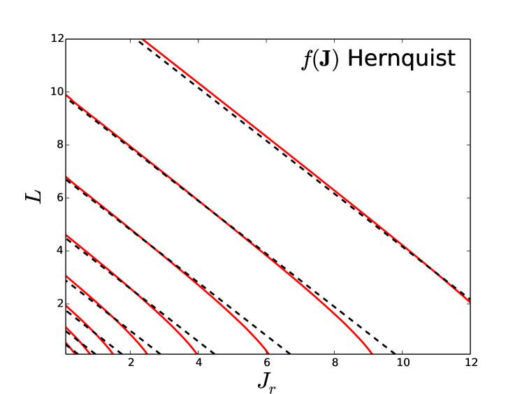
Figure 1: The red full curves show surfaces on which the DF  of the classical isotropic Hernquist sphere is constant in the $(J_{r},L)$ plane of action space, while the black dashed curves show surfaces on which the corresponding $f({\bf J})$ distribution function is constant.

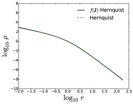
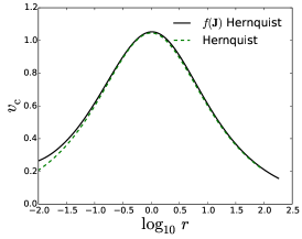
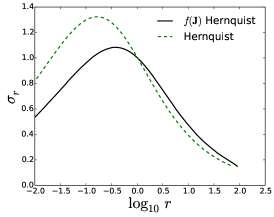
Figure 2: Density (left-hand panel), circular velocity (central panel), and radial velocity dispersion (left-hand panels) profiles for the classical isotropic Hernquist sphere (normalized to $r_{\rm b}$) and for the $f({\bf J})$ Hernquist model (normalized to $r_{0}$).

In Appendix A we derive an analytic expression for $J_{\rm r}=J_{\rm r}(H,L)$ in the spherical Hernquist potential. By numerically inverting this expression, we arrive at $H=H(J_{\rm r},L)$ for the Hernquist sphere. Combining this with the sphere’s ergodic DF, which was given already by Hernquist (1990), we have the exact $f=f[H({\bf J})]$. In Fig. 1 we show surfaces in action space on which this DF  is constant together with surfaces on which DF of the $f({\bf J})$ Hernquist model is constant. The differences are small but apparent and arise because the surfaces of constant energy are not exactly planar.

Fig. 2 compares the radial profiles of density, circular speed and radial component of velocity dispersion in the exact isotropic model and in the $f({\bf J})$ Hernquist model. The largest discrepancy is in the velocity dispersion and reflects the fact that the model is significantly radially biased around $r_{0}$. The long-dashed curve in Fig. 3 shows that the $f({\bf J})$ Hernquist model has a slight radial bias at all radii by plotting the anisotropy parameter

$$\beta_{\rm a}=1-{\sigma_{\phi}^{2}+\sigma_{z}^{2}\over 2\sigma_{r}^{2}}.$$ (39)

By virtue of the adopted form of $g$ (equation 35), $\beta_{\rm a}\to 0$ in the Keplerian regime. Even though the potential is not harmonic at the centre, still the model tends to isotropy also at small radii, which justifies our simple choice for $h({\bf J})$.

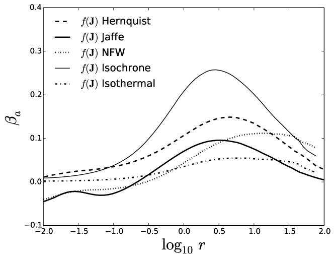
Figure 3: Anisotropy profiles for $f({\bf J})$ Hernquist, $f({\bf J})$ Jaffe, $f({\bf J})$ NFW, $f({\bf J})$ isochrone and $f({\bf J})$ isothermal models. The profiles are normalized to $r_{0}$ (eq.  38).

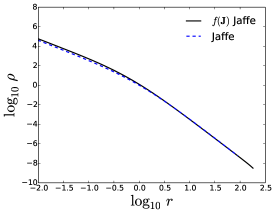
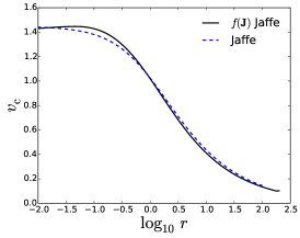
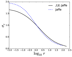
Figure 4: Same as Fig.  2, but for the classical isotropic Jaffe sphere and for the $f({\bf J})$ Jaffe model.

3.2.2 The Jaffe model

The Jaffe (1983) model behaves as Hernquist’s at large radii, while tending to $\rho\propto r^{-2}$ close to the centre. Fig. 4 shows the radial profiles of the $f({\bf J})$ Jaffe model defined by setting $(\alpha,\beta)=(2,4)$ in the DF (34), and compares them with the classical isotropic model. The discrepancies in $\sigma_{r}$ are due to the slight radial bias of the $f({\bf J})$ model around $r_{0}$. The full curve in Fig. 3 shows that this bias actually quite mild – $|\beta_{\rm a}|<0.1$.

3.2.3 NFW halo

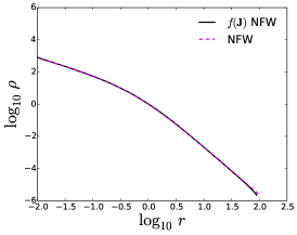
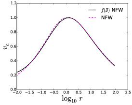
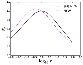
Figure 5: Same as Fig.  2, but for the classical isotropic NFW sphere and for the $f({\bf J})$ NFW model defined by equation (41).

The NFW model has $\beta=3$ with the consequence that its mass diverges logarithmically as $r\to\infty$ and its potential is never Keplerian. Consequently, the reasoning used to construct a DF above equation (34) does not apply. If we nevertheless adopt equation (34) with $(\alpha,\beta)=(1,3)$, we obtain a DF that implies that as $J\to\infty$ the mass with actions less than $J$ diverges like $\log J$. Asymptotically the circular speed of the standard NFW model is

$$v_{\rm c}\sim\sqrt{{\log(1+r/r_{0})\over r}},$$ (40)

so in this model the action of a circular orbit is $J_{\phi}\sim\sqrt{r\log r}$. This shows that mass diverging like $\log J$ in action space corresponds, to leading order, to divergence of the mass in real space like $\log r$. Hence it is plausible that the DF (34) with $(\alpha,\beta)=(1,3)$ generates a model similar to the NFW model.

Computation of $\rho(r)$ for the $f({\bf J})$ model with $(\alpha,\beta)=(1,3)$ bears out this expectation. However the slope of the model’s density profile at large $r$ is slightly steeper than desired, and a better fit to the classical NFW profile is obtained by adopting

$$f({\bf J})={M_{0}\over J_{0}^{3}}{[1+J_{0}/h({\bf J})]^{5/3}\over[1+g({\bf J})/J_{0}]^{2.9}}.$$ (41)

Fig. 5 shows the radial profiles of the classical NFW model and those of the model generated by the DF (41), which we shall call $f({\bf J})$ NFW model. The dotted curve in Fig. 3 shows that this model is mildly radially biased at radii larger than $r_{0}$ and it becomes very slightly tangentially biased for $r<r_{0}$. These anisotropies account for the difference between the $\sigma_{\rm r}$ profiles of the $f({\bf J})$ and classical NFW models.

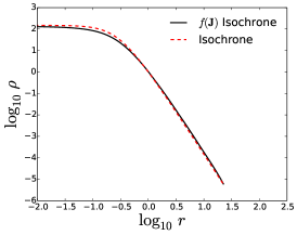
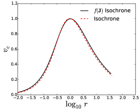
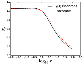
Figure 6: Same as Fig.  2, but for the classical isotropic isochrone sphere and for the $f({\bf J})$ isochrone model.

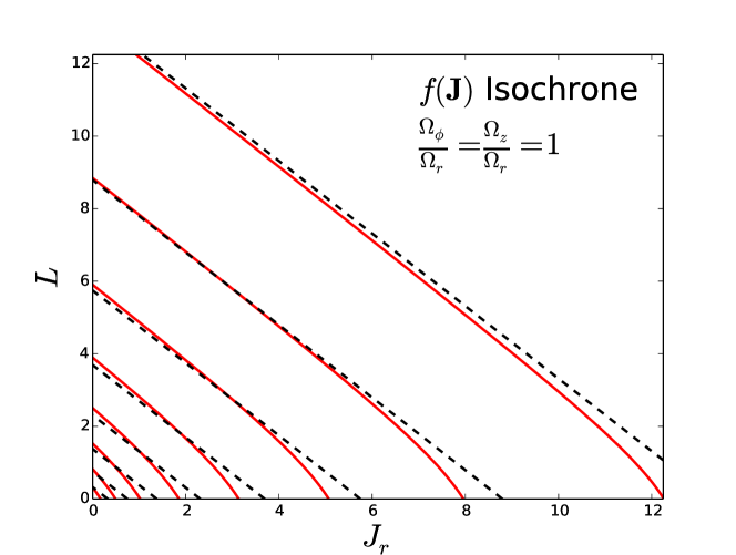
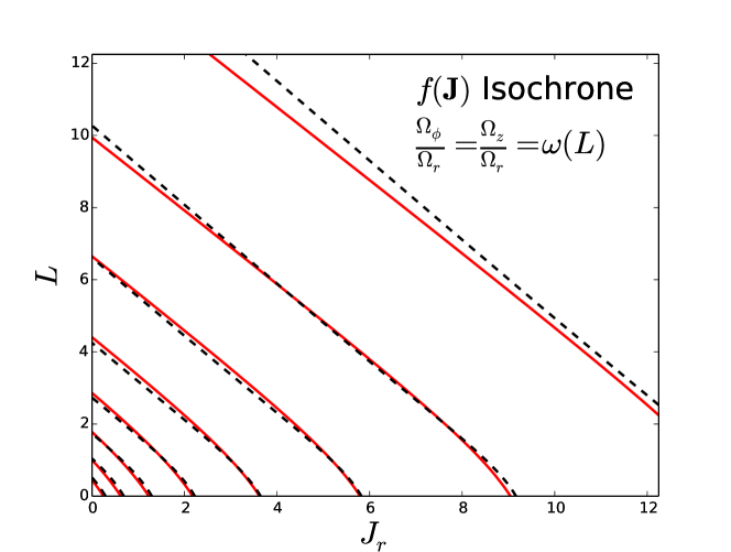
Figure 7: Surfaces of constant $H({\bf J})$ (red) and of constant $f({\bf J})$ black in action space for two $f({\bf J})$ isochrone models with different choice of the function $g$ appearing in the DF (42). In the upper panel $g$ is $J_{r}+L$ whereas in the lower panel it is $J_{r}+(\Omega_{\phi}/\Omega_{r})L$ where the frequency ratio is a function of $L$.

4 Cores and cuts

In the last section we addressed the problematic nature of power-law models – that their mass diverges at either small or large radii – by introducing separate slopes of the dependence of $f$ on ${\bf J}$ at small and large ${\bf J}$. The recovered models had central density cusps similar to those of the Hernquist, Jaffe and NFW models. If a homogeneous core is required, the natural DF to adopt is

$$f({\bf J})={M_{0}\over J_{0}^{3}}{1\over[1+g({\bf J})/J_{0}]^{2\beta-3}},$$ (42)

for then the phase-space density has the finite value $M_{0}/J_{0}^{3}$ at the centre of the model, and the asymptotic density profile is expected to be $\rho\propto r^{-\beta}$. For $\beta\leq 3$ the system has infinite mass, so for these models we taper the DF by subtracting a constant from the value given by equation (42)

$$f({\bf J})\mapsto f^{\prime}({\bf J})=\max\left[0,f({\bf J})-f({\bf J}_{\rm t})\right],$$ (43)

where ${\bf J}_{\rm t}$ is some large action, which defines a truncation radius

$$r_{\rm t}={|{\bf J}_{\rm t}|^{2}\over GM}.$$ (44)

4.1 Isochrone model

Fig. 6 compares the density profiles of the model equation (42) generates for $\beta=4$ (black curves) with those of the isochrone (Hénon, 1960). The two models are extremely similar, so we shall refer to the model generated by the DF (42) when $\beta=4$ as the $f({\bf J})$ isochrone model. The density profiles of the two models are essentially identical, but at $r\simeq r_{0}$ $\sigma_{r}$ is slightly smaller in the $f({\bf J})$ isochrone than in the classical isochrone because the $f({\bf J})$ isochrone is mildly radially biased near $r_{0}$ – the thin full curve in Fig. 3 shows $\beta_{\rm a}(r)$ for this model. It is non-zero because in action space surfaces of $f({\bf J})$ do not quite coincide with surfaces of constant $H({\bf J})$, as the upper panel of Fig. 7 shows by plotting contours of $f$ and $H$. For the isochrone potential we have an analytic expression for the frequency ratio $\Omega_{\phi}/\Omega_{r}$ as a function of $L$. The lower panel of Fig. 7 shows that the constant-energy and constant-DF contours are more closely aligned when the argument of the homogeneous function uses the exact frequency ratio.

Given that the exact DF of the isochrone is a complicated function of ${\bf J}$, it is astonishing that the trivial DF (42) provides such a good approximation to it.

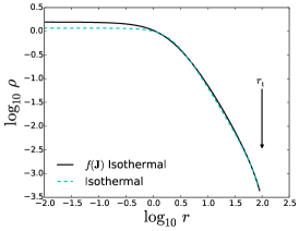
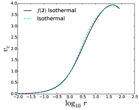
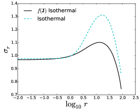
Figure 8: Same as Fig.  2, but for the truncated isotropic cored isothermal sphere (equation 46) and for the $f({\bf J})$ truncated isothermal model. We show the location of the truncation radius defined by equation (44).

4.2 Cored isothermal sphere

In Section 2.1 we derived an approximation (24) to the DF of the singular isothermal sphere. Here we modify this model into one that is numerically tractable by (i) adding a core, and (ii) tapering its density at large radii so the model’s mass becomes finite. Then the DF is

$$f({\bf J})={M_{0}\over J_{0}^{3}}\max\left(0,[1+J_{0}/h({\bf J})]^{2}-{[1+J_{0}/h({\bf J}_{\rm t})]^{2}}\right),$$ (45)

where $h({\bf J})$ is given by equation (10) with both frequency ratios set to $1/\surd 2$ and ${\bf J}_{\rm t}=(0,v_{\rm c}r_{\rm t},0)$. As full curves in Fig. 8 show, this DF generates a model that has a core that extends to $r_{0}$ and a density profile that plunges to zero near the truncation radius $r_{\rm t}$. The short-dashed curve in Fig. 3 shows the model’s anisotropy parameter $\beta_{\rm a}$, which is always small ($|\beta_{\rm a}|<0.04$).

An ergodic model with a simple functional form of $\rho(r)$ to which we can compare our $f({\bf J})$ model has

$$\rho(r)={v_{\rm c}^{2}\over 2\pi G(r^{2}+r_{\rm b}^{2})}{\rm e}^{-r^{2}/r_{\rm t}^{2}}.$$ (46)

The dashed curve in the left panel-hand of Fig. 8 shows that the model defined by the DF (46) provides an excellent fit to the density profile of our $f({\bf J})$ model. Curiously, in the $f({\bf J})$ model $\sigma_{r}(r)$ is more nearly constant within $r_{\rm t}$ than in either of the models with analytic density profiles. The dashed curve in the right-hand panel of Fig. 8 shows that the model defined by the DF (46) has a significantly deeper central depression in $\sigma_{r}$ than the $f({\bf J})$ model.

5 Conclusions

Studies of both our own and external galaxies will benefit from the availability of a flexible array of dynamical models of galactic components such as disc, bulge and dark halo. The construction of general models of this type is rather straightforward when one decides to start from an expression for the component’s DF as a function of the action integrals $J_{i}$. In this paper we have illustrated this fact by deriving simple analytic forms for DFs that self-consistently generate models that closely resemble the isochrone, Hernquist, Jaffe, NFW and truncated isothermal models. In previous papers Binney (2010, 2012b) has given simple analytic DFs that provide excellent fits to the structure of the Galactic disc, so now DFs are available for all commonly occurring galactic components.

Our models are tailored to minimise velocity anisotropy at both small and large radii. In all of them the anisotropy parameter $\beta_{\rm a}$ peaks at intermediate radii. The peak is by far sharpest in the $f({\bf J})$ isochrone, but even in this model $\beta_{\rm a}$ stays below $0.25$.

Our presentation has been elementary in the sense that we have confined ourselves to spherical, almost isotropic components that live in isolation. However, B14 showed that given a near-ergodic DF $f({\bf J})$ of a component such as those presented here, it is trivial to modify it so it generates a system that is flattened by velocity anisotropy, or by rotation, or by a combination of the two. Equally important, when the DF of an individual component is given as $f({\bf J})$, it is straightforward to add components. Such addition was exploited by Piffl et al. (2014) in a study of the contribution of dark matter to the gravitational force on the Sun: in that study the models fitted to data comprised a sum of DFs $f({\bf J})$ for the disc and the stellar halo. The dark halo was assigned a density distribution rather than a DF, but Piffl et al. (2015) represent the dark halo by the $f({\bf J})$ NFW model, making the Galaxy a completely self-consistent object. A key point for such work is that the mass of each component can be specified at the outset.

Our approach has several points of contact with that of Williams, Evans, & Bowden (2014) and Evans & Williams (2014), who derive approximations to $H({\bf J})$ for models that are defined by DFs of the form $f(E,L)$. In particular, they show that for their models better approximations to the iso-energy surfaces in action space can be obtained if one’s homogeneous function has as its argument the sum of a linear function of the actions, as used here, and a small term $\epsilon\sqrt{LJ_{r}}$. We expect that the anisotropy of our models could be enhanced by adding such a term.

In addition to assisting in the dynamical interpretation of observations of galaxies, the models that the present work makes possible could provide useful initial conditions for N-body simulations. The first step would be the construction of a self-consistent galaxy model from a judiciously chosen DF. Then one could Monte-Carlo sample the action space using the DF as the sampling density, and torus mapping (e.g. Binney & McMillan, 2011) could be used to generate an orbital torus at each of the selected actions. Finally some number $n$ of initial conditions $({\bf x},{\bf v})$ would be selected on each torus, uniformly space in the angles $\theta_{i}$. The resulting simulation would be in equilibrium to whatever precision had been used in the solution of Poisson’s equation, and it would experience a “cold start” (Sellwood, 1987). Moreover, given that it would be possible to evaluate the original DF at any phase-space point, the model would lend itself to the method of perturbation particles (Leeuwin et al., 1993) in which the simulation particles represent the difference between a dynamically evolving model and an underlying equilibrium rather than the whole model. This method has been little used in the past on account of the lack of interesting models with known DFs, which is precisely the need that we have here supplied.

Appendix A Analytical expression for the radial action in the Hernquist sphere

The radial action is defined as

$$J_{\rm r}=\frac{1}{2\pi}\oint p_{r}{\rm d}r={1\over\pi}\int_{r_{1}}^{r_{2}}{\rm d}r\,\sqrt{2E-2\Phi(r)-\frac{L^{2}}{r^{2}}},$$ (47)

where $\Phi(r)=-GM/(r+r_{\rm b})$ and $r_{1},r_{2}$ are the pericentric and apocentric radii for the given energy $E$ and angular momentum $L$, i.e., the two roots of the integrand in equation (47). Introducing the dimensionless quantities $s\equiv r/r_{\rm b}$, $\mathcal{E}\equiv-Er_{\rm b}/GM$ and $l=L/\sqrt{2GMr_{\rm b}}$, equation (47) can be rewritten get

$$J_{\rm r}=\frac{\sqrt{2GMr_{\rm b}}}{\pi}\int_{s_{1}}^{s_{2}}{\rm d}s\,\sqrt{-\mathcal{E}+\Psi(s)-\frac{l^{2}}{s^{2}}},$$ (48)

where $\Psi(s)\equiv 1/(1+s)$ is the relative dimensionless potential. We now change the integration variable variable from $s=(1-\Psi)/\Psi$ to $\Psi$ (Ciotti, 1996), and have

$$J_{\rm r}=\frac{\sqrt{2GMr_{\rm b}}}{\pi}\int_{\Psi_{2}}^{\Psi_{1}}{\rm d}\Psi\,\frac{\sqrt{\mathcal{P}(\Psi)}}{(1-\Psi)\Psi^{2}},$$ (49)

where $\Psi_{1}\equiv\Psi(s_{1})$, $\Psi_{2}\equiv\Psi(s_{2})$ and

$$\mathcal{P}(\Psi)=-\mathcal{E}(1-\Psi)^{2}+\Psi(1-\Psi)^{2}-l^{2}\Psi^{2}$$ (50)

is a cubic in $\Psi$, the roots of which can be found by standard methods (e.g., Dickson, 1914). $\Psi_{1},\Psi_{2}$ are two roots in the physical range $0\leq\Psi\leq 1$. Let $A$ be the third real root, so

$$\mathcal{P}(\Psi)=(\Psi_{1}-\Psi)(\Psi-\Psi_{2})(A-\Psi).$$ (51)

While it is physically obvious that two of the three real solutions of equation (50) are in the range $(0,1)$ and the remaining one is outside $(A>1)$, we remark that the same conclusion can be reached by purely algebraic arguments by using the Routh-Hurwitz theorem (see e.g., Gantmacher, 1959). By evaluating equations (50) and (51) at $\Psi=0$ one gets $A=\mathcal{E}/\Psi_{1}\Psi_{2}>0$. By splitting into its partial fractions the integrand in equation (49), it is possible to express the integral for $J_{\rm r}$ in terms of complete elliptic integrals (see Byrd and Friedman, 1971):

$$\begin{array}[]{l}\displaystyle J_{r}=\frac{\sqrt{2GMa}}{\pi}D_{5}\left[D_{1}\Pi\left(\alpha_{1},k^{2}\right)+D_{2}{\rm E}\left(k^{2}\right)+\right.\\ \\ \displaystyle\quad\left.+D_{3}{\rm K}\left(k^{2}\right)+D_{4}\Pi\left(\alpha_{2},k^{2}\right)\right],\end{array}$$ (52)

where ${\rm K},{\rm E},\Pi$ are respectively the complete elliptic integral of the first, second and third kind,

$$\alpha_{1}\equiv\frac{\Psi_{1}-\Psi_{2}}{\Psi_{2}},\quad\alpha_{2}\equiv\frac{\Psi_{1}-\Psi_{2}}{1-\Psi_{2}},\quad k^{2}\equiv\frac{\Psi_{1}-\Psi_{2}}{A-\Psi_{2}}$$ (53)

and finally

$$\begin{array}[]{l}\displaystyle D_{1}=[(1-2\Psi_{1})\Psi_{2}+\Psi_{1}]A+\Psi_{1}\Psi_{2},\\ \displaystyle D_{2}=\Psi_{2}(\Psi_{2}-A),\\ \displaystyle D_{3}=\Psi_{2}(A-2),\\ \displaystyle D_{4}=2\Psi_{2}(A-1)(\Psi_{1}-1),\\ \displaystyle D_{5}=-\sqrt{A-\Psi_{2}}/D_{2}.\end{array}$$ (54)

We have tested the formula (52) for consistency by numerically integrating equation (47) for a large set of orbits at different $(E,L)$ and the numerical and analytical results agree within the error of the employed routine.

References

- Arnold (1978) Arnold V.I., 1978, The Mathematical Methods of Classical Mechanics, Springer, New York
- Binney (2010) Binney J., 2010, MNRAS, 401, 231
- Binney (2012a) Binney J., 2012a, MNRAS, 426, 1324
- Binney (2012b) Binney J., 2012b, MNRAS, 426, 1328
- Binney & McMillan (2011) Binney J., McMillan P.J., 2011, MNRAS, 413, 1889
- Binney (2014) Binney J., 2014, MNRAS, 440, 787 (B14)
- Binney & Tremaine (2008) Binney, J., & Tremaine, S. 2008, Galactic Dynamics, 2nd edn. Princeton Univ. Press, Princeton, NJ
- Byrd and Friedman (1971) Byrd P.F., Friedman M. D., 1971, Handbook of elliptic integrals for engineers and scientists, Springer-Verlag, Berlin
- Ciotti (1996) Ciotti L., 1996, ApJ, 471, 68
- Dehnen (1993) Dehnen W., 1993, MNRAS, 265, 250
- Dickson (1914) Dickson L.E., 1914, Elementary Theory of Equations, J. Wiley & Sons Incorporated, Hoboken, New Jersey, USA
- Eddington (1916) Eddington A. S., 1916, MNRAS, 76, 572
- Evans (1994) Evans N. W., 1994, MNRAS, 267, 333
- Evans & Williams (2014) Evans N. W., Williams A. A., 2014, MNRAS, 443, 791
- Fermani (2013) Fermani F., 2013, DPhil Thesis, University of Oxford
- Gantmacher (1959) Gantmacher F.R., 1959, The Theory of Matrices Vol.2, American Mathematical Society, Providence, Rhode Island, USA
- Gerhard & Saha (1991) Gerhard O.E., Saha P., 1991, MNRAS, 251, 449
- Hénon (1960) Hénon M., 1960, AnAp, 23, 474
- Hernquist (1990) Hernquist L., 1990, ApJ, 356, 359
- Jaffe (1983) Jaffe W., 1983, MNRAS, 202, 995
- Jeans (1915) Jeans J. H., 1915, MNRAS, 76, 70
- Leeuwin et al. (1993) Leeuwin F., Combes F., Binney J., 1993, MNRAS, 262, 1013
- Navarro, Frenk, & White (1996) Navarro J. F., Frenk C. S., White S. D. M., 1996, ApJ, 462, 563
- Piffl et al. (2014) Piffl T., et al., 2014, MNRAS, 445, 3133
- Piffl et al. (2015) Piffl T., Penoyre Z., Binney J., 2015, MNRAS, to be submitted
- Prendergast & Tomer (1970) Prendergast K.H., Tomer E., 1970, AJ, 75, 647
- Rowley (1988) Rowley G., 1988, ApJ, 331, 124
- Sanders & Binney (2014) Sanders J.L., Binney J., 2014, MNRAS, 441, 3284
- Sanders & Binney (2015) Sanders J.L., Binney J., 2015, MNRAS, in press
- Sellwood (1987) Sellwood J.A., ARA&A, 25, 151
- Williams, Evans, & Bowden (2014) Williams A. A., Evans N. W., Bowden A. D., 2014, MNRAS, 442, 1405
- Wilson (1975) Wilson C.P., 1975, ApJ, 80, 175