Activation of effector immune cells promotes tumor stochastic extinction: A homotopy analysis approach

Abstract

In this article we provide homotopy solutions of a cancer nonlinear model describing the dynamics of tumor cells in interaction with healthy and effector immune cells. We apply a semi-analytic technique for solving strongly nonlinear systems - the Step Homotopy Analysis Method (SHAM). This algorithm, based on a modification of the standard homotopy analysis method (HAM), allows to obtain a one-parameter family of explicit series solutions. By using the homotopy solutions, we first investigate the dynamical effect of the activation of the effector immune cells in the deterministic dynamics, showing that an increased activation makes the system to enter into chaotic dynamics via a period-doubling bifurcation scenario. Then, by adding demographic stochasticity into the homotopy solutions, we show, as a difference from the deterministic dynamics, that an increased activation of the immune cells facilitates cancer clearance involving tumor cells extinction and healthy cells persistence. Our results highlight the importance of therapies activating the effector immune cells at early stages of cancer progression.

I Introduction

Exact solutions for nonlinear equations are difficult to obtain, and a handful of novel methods and techniques, either analytical or numerical, have been developed. The nature of the interactions in biological systems gives place to nonlinear dynamics that can generate, for some parameter values, very complicated dynamics e.g. chaos. Hence, advances to better characterize the dynamics for nonlinear systems turn out to be extremely useful to analyze and understand such systems. As far as analytical approaches are concerned, various perturbation techniques are frequently applied in science and engineering, and they do help us to enhance our understanding of nonlinear phenomena. Nevertheless, many perturbation methods are only valid and effective for weakly nonlinear problems, due to their strongly dependence upon small/large physical parameters. On the other hand, the so called traditional non-perturbation methods, such as the artificial small parameter method Lyap1992 , the $\delta$-expansion method Karm1990 ; Awr1998 , and the Adomian’s decomposition method Adomian1976 ; Adomian1991 ; Rach1984 ; Adomian1984a , are known to be formally independent of small/large physical parameters. However, all of these non-perturbation techniques are, in fact, valid for weakly nonlinear problems and they can not ensure the convergence of solutions series for strongly nonlinear systems. As a consequence, in recent years there has been a growing interest in obtaining continuous solutions for nonlinear dynamical systems by means of analytical or semi-analytical techniques. The homotopy analysis method (HAM), initially proposed by Liao Liao1992 ; Liao2003 , can be used to obtain convergent series solutions of strongly nonlinear problems (including e.g., ordinary differential equations, partial differential equations, algebraic equations, and differential-integral equations).

Unlike perturbation methods, the HAM is independent of small/large physical parameters. Differently from perturbation and non-perturbation methods, the HAM is valid even for strongly nonlinear problems and it is characterized by two central aspects: (i) a great freedom to choose proper linear operators and base functions to approximate a nonlinear problem, and (ii) the use of an artificial parameter that represents a simple way to adjust and control the convergence region and rate of convergence of the series solution. Based on homotopy, a fundamental concept in topology and differential geometry Sen1983 , the HAM allows us to construct a continuous mapping of an initial guess approximation to the exact solutions of the considered equations, using a chosen linear operator. Indeed, the method enjoys considerable freedom in choosing auxiliary linear operators. The HAM represents a truly significant milestone that converts a complicated nonlinear problem into an infinite number of simpler linear sub-problems Liao2007 . Since Liao’s work Liao2003 , the HAM has been successfully employed in the fractional Lorenz system Alomari2010 , in fluid dynamics Hayat2005 , in the Fitzhugh-Nagumo model Li2006 , as well as to obtain soliton solutions also for the Fitzhugh-Nagumo system Abbasbandy2008 . This semi-analytical technique has been also used in complex systems in ecology Arafa2011 ; Putcha2012 , in epidemiology Liao2009 , as well as in models of interactions between tumors and oncolytic viruses Usha2012 .

In the present article we apply the HAM to obtain solutions of a cancer growth model proposed by Itik and Banks Itik2010 . Such a model, based on Volterra-Lotka predator-prey dynamics, describes the interactions between tumor, healthy, and effector immune cells (CD8 T cells i.e., cytotoxic lymphocytes, CTLS). Predator-prey or competition Volterra-Lotka systems are known to display deterministic chaos for systems with three or more dimensions Hastings1991 ; Vano2006 ; Gakkhar2003 ; Tang2002 . Together with the model by Itik and Banks, several other theoretical models have addressed the dynamics of cancer and tumor cells Kuznetsov1994 ; dePillis2003 ; Kirschner1998 . Interestingly, the model by Itik and Banks can be considered as being qualitatively validated with experimental data, because its parameter values were chosen to match with some biological evidences. This model could be thus considered as being qualitatively validated with experimental data dePillis2003 ; Letellier2013 . Motivated by the characterization of chaos provided by Itik and Banks, a collection of questions pertaining to chaotic tumor behavior in terms of symbolic dynamics and predictability as well as to the control of healthy cells behavior corresponding to physiological relevant parameter regions, have been recently addressed in Refs. Duarte2013 and Duarte2014 , respectively. In fact, chaos in tumor dynamics and its property of sensitivity to initial conditions have been suggested to have numerous analogies to clinical evidences Denis2012a ; Denis2012b .

Numerical algorithms have been extremely important to investigate complex dynamical systems such as cancer. However, they allow us to analyze the dynamics at discrete points only, thereby making impossible to obtain continuous solutions. By means of the HAM, accurate approximations allow a good semi-analytical description of the time variables, making also possible to use the homotopy solutions to explore the model dynamics, as well as to investigate possible scenarios of tumor clearance, either deterministic or stochastic. This is the aim that we pursue in this contribution. Specifically, we will calculate the homotopy solutions of the cancer model by means of the step homotopy analysis method (SHAM, see Alomari2010 ). Then, the homotopy solutions will be used to explore the effect of a key parameter in the population dynamics: the activation of the immune system cells due to tumor antigen recognition, given by parameter $r_{3}$ (see next Section). As we will show, the system is very sensitive to this parameter, and its change can involve the shift from order to chaos. This key parameter is especially interesting because modulates the response of the immune system against tumor cells and, as we will show, the dynamics is especially sensitive to $r_{3}$. Despite its importance, the dependence of the dynamics of the model under investigation on $r_{3}$ remains poorly explored (see Duarte2014 for the analysis of a narrow range of $r_{3}$ values within the framework of chaotic crises and chaos control). Moreover, the impact of this parameter on possible extinction scenarios of tumor cells due to demographic fluctuations has, as far as we know, not being investigated. Interestingly, several therapeutic methods, that will be discussed in this article, are currently available to clinically manipulate this parameter, thus being a realistic candidate to fight against tumor progression.

Finally, we will use the homotopy solutions to investigate the role of demographic stochasticity in the dynamics of the model, paying special attention to the role of noise in potential scenarios of tumor clearance and persistence of healthy cells due to changes in the activation levels of effector immune cells.

II Cancer mathematical model

In this article we analyze a cancer mathematical model initially studied by Itik and Banks Itik2010 . The model describes the dynamics of three interacting cell populations: tumor cells, healthy cells and effector immune cells i.e., CD8 cytotoxic T-cells, CTLs. Effector cells are the relative short-lived activated cells of the immune system that defend the body in an immune response. Similarly to previous cancer models Kuznetsov1994 ; dePillis2003 ; Kirschner1998 ; Kuznetsov2001 ; dePillis2006 ; Itik2009 ; Baizer1996 , this model describes the competition dynamics of these three interacting cell types in a well-mixed system (e.g., liquid cancers such as leukemias or multiple lymphomas). Among several biologically-meaningful assumptions (see Itik2010 ), the model assumes that the antitumor effect of the immune system response is carried out by cytotoxic T-cells i.e., mediated by the T-cell based adaptive arm. Alpha-beta T-cells are activated upon recognition of their cognate tumor specific antigens by the cell surface T-Cell Receptor (TCR) in the form of small peptides presented in the context of the major histocompatibility complex (MHC) molecules. CD8 T-cells are responsible for direct cell mediated cytotoxicity following activation by antigen presenting cells (APCs) and are thought to be central players in the anti-tumor immune response. To achieve full activation, the signal emanating from the TCR has to be enhanced by messages sent by costimulatory molecules such as CD28 also present in the surface of the T-cell. Failure of the engagement of costimulatory proteins, activation of coinhibitory receptors such as CTLA-4 or PD-1 or the presence of CD4 regulatory ($T_{reg}$) T cells may lead to the failure of the activation of the T-cell or to the downregulation of the immune response. Disarming these inhibitory mechanisms off may lead to the reactivation of the antitumor immune response and to supraphysiological levels of T-cell activation useful in the clinical setting (see Discussion Section).

In order to simplify the mathematical analysis, the initial model was non-dimensionalized Itik2010 . The scaled resulting system of differential equations is given by:

$$\frac{dx_{1}}{dt}=x_{1}\left(1-x_{1}\right)-a_{12}x_{1}x_{2}-a_{13}x_{1}x_{3},$$ (1)

$$\frac{dx_{2}}{dt}=r_{2}x_{2}\left(1-x_{2}\right)-a_{21}x_{1}x_{2},$$ (2)

$$\frac{dx_{3}}{dt}=\frac{r_{3}x_{1}x_{3}}{x_{1}+k_{3}}-a_{31}x_{1}x_{3}-d_{3}x_{3}.$$ (3)

The variables $x_{1}$, $x_{2}$ and $x_{3}$ denote, respectively, the population numbers of tumor cells, healthy cells and effector immune cells against their specific maxima carrying capacities $k_{1}$, $k_{2}$ and $k_{3}$ (see Section 4 in Itik2010 ). Parameter $a_{12}$ is the tumor cells inactivation rate by the healthy cells; $a_{13}$ is the tumor cells inactivation rate by the effector cells; $r_{2}$ is the intrinsic growth rate of the healthy tissue cells; $a_{21}$ is the healthy cells inactivation rate by the tumor cells; $r_{3}$ corresponds to the activation rate of effector cells due to tumor cells’ antigen recognition; $a_{31}$ is the effector cells inactivation rate by the tumor cells. Finally, $d_{3}$ is the density-dependent death rate of the effector cells (see Itik2010 for a detailed description of the model parameters).

We want to notice that the inactivation rate (or the elimination rate) of tumor cells by the action of the effector immune cells (modeled with the last term in Eq. (1)) is assumed to be proportional to the number of effector immune cells, and no saturation is considered. A mechanism of elimination of tumor cells is given by the release of cytotoxic granules by the effector cells that impair or destroy tumor cells. Effector cells can clonally expand after antigen recognition, so the model assumes that they can be present in excess if needed. Hence, no saturation is considered for this term. The activation of effector immune cells due to antigen recognition used in the first term of Eq. (3) can be viewed as a Holling-II functional response, typically used to model predator feeding saturation in ecological dynamical systems. For our system, it is assumed a decelerating activation rate at increasing number of tumor cells since the activation of effector immune cells is limited by their requirement to recognize the tumor antigens in the context of the Antigen Presenting Cells (APCs). In this case, a process of cell-cell interaction and receptor recognition is required between APCs and tumor cells prior to activation, and thus an increasing number of tumor cells does not necessarily involve an increasing activation of effector cells.

The dynamics of this model is very rich, and both ordered (e.g., stable points or periodic orbits) and disordered (i.e., chaos) dynamics can be found for different parameter values Itik2010 ; Duarte2013 .

The model parameters will be fixed, if not otherwise specified, following Itik2010 , i.e., $a_{12}=1$; $a_{21}=1.5$; $d_{3}=0.5$; $k_{3}=1$; $r_{2}=0.6$; $a_{13}=2.5$; $a_{31}=0.2$. This set of parameter values can involve chaos for a wide range of $r_{3}$ values (see below).

III Homotopy analysis method

As in the cancer model explored in this article, many practical situations can be modeled with different types of systems of ordinary differential equations of the form

$$\overset{.}{x}_{i}=f_{i}\left(t,x_{1},...,x_{n}\right),\text{ }x_{i}(t_{0})=x_{i,0},\text{ }i=1,2,...,n.$$ (4)

Firstly, according to homotopy analysis method (HAM) Liao2003 , each equation of the system (4) is written in the form

$$N_{i}\left[x_{1}(t),x_{2}(t)...,x_{n}(t)\right]=0,\text{ }i=1,2,...,n,$$

where $N_{1},N_{2},...,N_{n}$ are nonlinear operators, $t$ denotes the independent variable and $x_{1}(t),x_{2}(t)...,x_{n}(t)$ are the unknown functions. From a generalization of the traditional homotopy method, Liao has stablished in Liao2003 the so-called zeroth-order deformation equation

$$\left(1-q\right)L\left[\phi_{i}\left(t;q\right)-x_{i,0}(t)\right]=qh_{0}N_{i}\left[\phi_{1}\left(t;q\right),...,\phi_{n}\left(t;q\right)\right],$$ (5)

where $q\in\left[0,1\right]$ is an embedding parameter, $h_{0}$ is a non-zero auxiliary artifitial parameter, $L$ is an auxiliary linear operator, $x_{i,0}(t)$ are initial guesses and $\phi_{i}\left(t;q\right)$ are unknown functions. It is important to emphasize that, in the frame of HAM, there is a great freedom to choose auxiliary entities such as $h_{0}$, $L$ and base functions for the representation of the solution $x_{i}(t)$. Specifically, we can use in the construction of the solution $x_{i}(t)$ base functions such as polynomials, exponentials, rational functions, etc. It is obvious that when $q=0$ and $q=1$, both

$$\phi_{i}\left(t;0\right)=x_{i,0}(t)\text{ and }\phi_{i}\left(t;1\right)=x_{i}(t)$$

hold. According to (5), as $q$ increases from $0$ to $1$, the function $\phi_{i}\left(t;q\right)$ varies from the initial guess $x_{i,0}(t)$ to the solution $x_{i}(t)$. Expanding $\phi_{i}\left(t;q\right)$ in Taylor series with respect to $q$, we obtain

$$\phi_{i}\left(t;q\right)=x_{i,0}(t)+\sum\limits_{m=1}^{+\infty}x_{i,m}(t)q^{m},$$ (6)

where

$$x_{i,m}(t)=\left.\frac{1}{m!}\frac{\partial^{m}\phi_{i}\left(t;q\right)}{\partial q^{m}}\right|_{q=0}.$$ (7)

As stated by Liao Liao2003 , if the auxiliary linear operators, the base functions and the auxiliary parameter $h_{0}$ are properly chosen, then the series (6) converges at $q=1$ and

$$x_{i}(t)=\phi_{i}\left(t;1\right)=x_{i,0}(t)+\sum\limits_{m=1}^{+\infty}x_{i,m}(t),$$

which is one of the solutions of the original nonlinear equations. Taking the $m^{th}$-order homotopy-derivative of the $zero^{th}$-order Eqs. (5), and using the corresponding properties, we have the $m^{th}$-order deformation equations

$$L\left[x_{i,m}(t)-\chi_{m}x_{i,m-1}(t)\right]=h_{0}R_{i,m}\left[x_{1,m-1}(t),...,x_{n,m-1}\left(t\right)\right],\text{ \ }i=1,2,...,n,$$ (8)

where

$$R_{i,m}\left[x_{1,m-1}(t),...,x_{n,m-1}\left(t\right)\right]=\left.\frac{1}{(m-1)!}\frac{\partial^{m-1}N_{i}\left[\phi_{1}\left(t;q\right),...,\phi_{n}\left(t;q\right)\right]}{\partial q^{m-1}}\right|_{q=0}$$

and

$$\chi_{m}=\left\{\begin{array}[]{c}0,\text{ \ }m\leq 1\\ \\ 1,\text{ \ }m>1\end{array}\right..$$

It is important to notice that each function $x_{i,m}(t)$ $(m\geq 1)$ is governed by the linear family of equations (8). This way the HAM converts a complicated nonlinear problem into simpler linear sub-problems. For some strongly nonlinear problems it is appropriate to use the step homotopy analysis method (SHAM). This analytical technique is based on a modification of the standard HAM, that we have just described, which allows us to obtain a one-parameter family of explicit series solutions in a sequence of intervals. For more details, we refer the reader to Ref. Alomari2010 (and references therein), where the SHAM is also explained in detail for the fractional Lorenz system. At this moment, after the previous considerations, we are able to apply the HAM and the SHAM for solving analytically the Itik-Banks cancer growth model.

Let us consider the Eqs. (1)-(3) subject to the initial conditions

$$x_{1}(0)=IC_{1},\text{ \ \ }x_{2}(0)=IC_{2},\text{ \ \ }x_{3}(0)=IC_{3}.$$

Following the HAM, it is straightforward to choose

$$x_{1,0}(t)=IC_{1},\text{ \ \ }x_{2,0}(t)=IC_{2},\text{ \ \ }x_{3,0}(t)=IC_{3},$$

as our initial approximations of $x_{1}(t),$ $x_{2}\left(t\right)$ and $x_{3}\left(t\right)$, respectively. In this work we will use $IC_{1}=0.13858...,$ $IC_{2}=0.69568...,$ $IC_{3}=0.01380...$. We choose the auxiliary linear operators

$$L\left[\phi_{i}\left(t;q\right)\right]=\frac{\partial\phi_{i}\left(t;q\right)}{\partial t}+\phi_{i}\left(t;q\right),$$

with the property $L\left[C_{i}e^{-t}\right]=0$, where $C_{i}$ are integral constants (hereafter $i=1,2,3$). The Eqs. (1)-(3) suggest the definition of the nonlinear operators $N_{1},$ $N_{2}$ and $N_{3}$ as

$$N_{1}\left[\phi_{1}\left(t;q\right),\phi_{2}\left(t;q\right),\phi_{3}\left(t;q\right)\right] = \frac{\partial\phi_{1}\left(t;q\right)}{\partial t}-\phi_{1}\left(t;q\right)+\phi_{1}^{2}\left(t;q\right)+a_{12}\phi_{1}\left(t;q\right)\phi_{2}\left(t;q\right)+$$

$$+a_{13}\phi_{1}\left(t;q\right)\phi_{3}\left(t;q\right),$$

$$N_{2}\left[\phi_{1}\left(t;q\right),\phi_{2}\left(t;q\right),\phi_{3}\left(t;q\right)\right]=\frac{\partial\phi_{2}\left(t;q\right)}{\partial t}-r_{2}\phi_{2}\left(t;q\right)+r_{2}\phi_{2}^{2}\left(t;q\right)+a_{21}\phi_{1}\left(t;q\right)\phi_{2}\left(t;q\right),$$

$$N_{3}\left[\phi_{1}\left(t;q\right),\phi_{2}\left(t;q\right),\phi_{3}\left(t;q\right)\right] = \phi_{1}\left(t;q\right)\frac{\partial\phi_{3}\left(t;q\right)}{\partial t}+k_{3}\frac{\partial\phi_{3}\left(t;q\right)}{\partial t}-r_{3}\phi_{1}\left(t;q\right)\phi_{3}\left(t;q\right)+$$

$$+a_{31}\phi_{1}^{2}\left(t;q\right)\phi_{3}\left(t;q\right)+a_{31}k_{3}\phi_{1}\left(t;q\right)\phi_{3}\left(t;q\right)+$$

$$+d_{3}\phi_{1}\left(t;q\right)\phi_{3}\left(t;q\right)+d_{3}k_{3}\phi_{3}\left(t;q\right).$$

If $q\in\left[0,1\right]$ and $h_{0}$ the non-zero auxiliary parameter, the $zero^{th}$-order deformation equations are of the following form

$$\left(1-q\right)L\left[\phi_{i}\left(t;q\right)-x_{i,0}(t)\right]=qh_{0}N_{i}\left[\phi_{1}\left(t;q\right),\phi_{2}\left(t;q\right),\phi_{3}\left(t;q\right)\right],$$ (9)

subject to the initial conditions

$$\phi_{1}\left(0;q\right)=0.13858...,\phi_{2}\left(0;q\right)=0.69568...,\text{ }\phi_{3}\left(0;q\right)=0.01380....$$

For $q=0$ and $q=1$, the above $zero^{th}$-order equations (9) have the solutions

$$\phi_{1}\left(t;0\right)=x_{1,0}(t),\text{ }\phi_{2}\left(t;0\right)=x_{2,0}(t),\text{ }\phi_{3}\left(t;0\right)=x_{3,0}(t)$$ (10)

and

$$\phi_{1}\left(t;1\right)=x_{1}(t),\text{ }\phi_{2}\left(t;1\right)=x_{2}(t),\text{ }\phi_{3}\left(t;1\right)=x_{3}(t).$$ (11)

When $q$ increases from $0$ to $1$, the functions $\phi_{1}\left(t;q\right)$, $\phi_{2}\left(t;q\right)$ and $\phi_{3}\left(t;q\right)$ vary from $x_{1,0}(t)$, $x_{2,0}(t)$ and $x_{3,0}(t)$ to $x_{1}(t)$, $x_{2}(t)$ and $x_{3}(t)$, respectively. Expanding $\phi_{1}\left(t;q\right)$, $\phi_{2}\left(t;q\right)$ and $\phi_{3}\left(t;q\right)$ in Taylor series with respect to $q$, we have the homotopy-Maclaurin series

$$\phi_{i}\left(t;q\right)=x_{i,0}(t)+\sum\limits_{m=1}^{+\infty}x_{i,m}(t)q^{m},$$ (12)

in which

$$x_{i,m}(t)=\left.\frac{1}{m!}\frac{\partial^{m}\phi_{i}\left(t;q\right)}{\partial q^{m}}\right|_{q=0},$$ (13)

where $h_{0}$ is chosen in such a way that these series are convergent at $q=1$. Thus, through Eqs (10)-(13), we have the homotopy series solutions

$$x_{i}(t)=x_{i,0}(t)+\sum\limits_{m=1}^{+\infty}x_{i,m}(t),$$ (14)

Taking the $m$th-order homotopy derivative of $zero$th-order Eqs. (9), and using the properties

$$D_{m}\left(\phi_{i}\right)=x_{i,m},\text{ }D_{m}\left(q^{k}\phi_{i}\right)=D_{m-k}\left(\phi_{i}\right)=\left\{\begin{array}[]{ll}x_{i,m-k},&\text{ \ \ }0\leq k\leq m\\ &\\ 0,&\text{ \ \ otherwise}\end{array}\right.,$$

$$D_{m}\left(\phi_{i}^{2}\right)=\sum\limits_{k=0}^{m}x_{i,m-k}~{}x_{i,k},$$

and

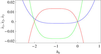
Figure 1: Samples of $h_{0}$-curves for the Itik-Banks system under $12^{th}$-order approximation for $t=0$, $a_{13}=5.0$, $a_{31}=1.3$ and $r_{3}=4.5$ (red - $\overset{\cdot}{x}_{1}\left(h_{0}\right)$, green - $\overset{\cdot}{x}_{2}\left(h_{0}\right)$ and blue - $\overset{\cdot}{x}_{3}\left(h_{0}\right)$).

$$D_{m}\left(\phi_{i}\psi_{i}\right)=\sum\limits_{k=0}^{m}D_{k}\left(\phi_{i}\right)~{}D_{m-k}\left(\psi_{i}\right)=\sum\limits_{k=0}^{m}x_{i,k}~{}y_{i,m-k},$$

where $D_{m}$ means the $m$th-order derivative in order to $q$, we obtain the $m^{th}$-order deformation equations

$$L\left[x_{i,m}(t)-\chi_{m}x_{i,m-1}(t)\right]=h_{0}R_{i,m}\left[x_{1,m-1}(t),x_{2,m-1}(t),x_{3,m-1}(t)\right],$$ (15)

with

$$\chi_{m}=\left\{\begin{array}[]{c}0,\text{ \ }m\leq 1\\ \\ 1,\text{ \ }m>1\end{array}\right.$$

and the following initial conditions

$$x_{1,m}(0)=0,\text{ }x_{2,m}(0)=0,\text{ }x_{3,m}(0)=0.$$ (16)

Defining the vector $\overrightarrow{x}_{m-1}=\left(x_{1,m-1}(t),x_{2,m-1}(t),x_{3,m-1}(t)\right),$

$$R_{1,m}\left[\overrightarrow{x}_{m-1}\right] = \overset{.}{x}_{1,m-1}(t)-x_{1,m-1}(t)+\sum\limits_{k=0}^{m-1}x_{1,m-1-k}(t)~{}x_{1,k}(t)+$$

$$a_{12}\sum\limits_{k=0}^{m-1}x_{1,k}(t)~{}x_{2,m-1-k}(t)+a_{13}\sum\limits_{k=0}^{m-1}x_{1,k}(t)~{}x_{3,m-1-k}(t),$$

$$R_{2,m}\left[\overrightarrow{x}_{m-1}\right] = \overset{.}{x}_{2,m-1}(t)-r_{2}x_{2,m-1}(t)+r_{2}\sum\limits_{k=0}^{m-1}x_{2,m-1-k}(t)~{}x_{2,k}(t)+$$

$$+a_{21}\sum\limits_{k=0}^{m-1}x_{1,k}(t)~{}x_{2,m-1-k}(t),$$

and

$$R_{3,m}\left[\overrightarrow{x}_{m-1}\right] = \sum\limits_{k=0}^{m-1}\left(x_{1,k}(t)\overset{.}{x}_{3,m-1-k}(t)\right)+k_{3}\overset{.}{x}_{3,m-1}(t)-$$

$$-r_{3}\sum\limits_{k=0}^{m-1}\left(x_{1,k}(t)~{}x_{3,m-1-k}(t)\right)+$$

$$+a_{31}\sum\limits_{k=0}^{m-1}\left[\left(\sum\limits_{j=0}^{k}x_{1,k-j}(t)~{}x_{1,j}(t)\right)x_{3,m-1-k}\right]+$$

$$+a_{31}k_{3}\sum\limits_{k=0}^{m-1}\left(x_{1,k}(t)~{}x_{3,m-1-k}(t)\right)+d_{3}\sum\limits_{k=0}^{m-1}\left(x_{1,k}(t)~{}x_{3,m-1-k}(t)\right)+$$

$$+d_{3}k_{3}x_{3,m-1}(t).$$

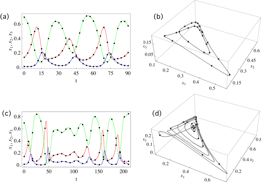
Figure 2: Comparison between the homotopy solutions (solid lines) obtained with the Step Homotopy Analysis Method (SHAM) developed in Section 3, and the numerical simulations (black dots) for Eqs. (1)-(3). Time series of the dynamical variables [$x_{1}$ (red), $x_{2}$ (green) and $x_{3}$ (blue)], and the corresponding attractors, represented in the phase space ($x_{1},x_{2},x_{3}$). In (a) and (b) we display the period 2 dynamics, using $a_{13}=5$, $a_{31}=1.3$, and $r_{3}=4$. In (c) and (d) we show the chaotic attractor obtained setting $(a_{13},a_{31},r_{3})=(5,0.9435,4.5)$.

Proceeding in this way, it is easy to solve the linear non-homogeneous Eqs. (15) at initial conditions (16) for all $m\geq 1$, obtaining:

$$x_{i,m}(t)=\chi_{m}~{}x_{i,m-1}(t)+h_{0}~{}e^{-t}\int\limits_{0}^{t}e^{\tau}R_{i,m}\left[\overrightarrow{x}_{m-1}\right]d\tau,$$ (20)

As an example, for $m=1$, we have:

$$x_{1,1}(t) = 0.13858-0.119376h_{0}+0.0964073a_{12}h_{0}+0.0019124a_{13}h_{0}+0.119376e^{-t}h_{0}-$$

$$-0.0964073a_{12}e^{-t}h_{0}-0.0019124a_{13}e^{-t}h_{0},$$

$$x_{2,1}(t) = 0.69568+0.0964073a_{21}h_{0}-0.0964073a_{21}e^{-t}h_{0}-0.211709h_{0}r_{2}+0.211709e^{-t}h_{0}r_{2},$$

$$x_{3,1}(t) = 0.0138+0.000265021a_{31}h_{0}+0.0019124d_{3}h_{0}-0.000265021a_{31}e^{-t}h_{0}-$$

$$-0.0019124d_{3}e^{-t}h_{0}+0.0019124a_{31}h_{0}k_{3}+0.0138d_{3}h_{0}k_{3}-$$

$$-0.0019124a_{31}e^{-t}h_{0}k_{3}-0.0138d_{3}e^{-t}h_{0}k_{3}-0.0019124h_{0}r_{3}+$$

$$+0.0019124e^{-t}h_{0}r_{3}.$$

It is straightforward to obtain terms for other values of $m$. In order to have an effective analytical approach of Eqs. (1)-(3) for higher values of $t$, we use the step homotopy analysis method, in a sequence of subintervals of time step $\Delta t$ and the $12^{th}$-order HAM approximate solutions of the form:

$$x_{i}(t)=x_{i,0}(t)+\sum\limits_{m=1}^{11}x_{i,m}(t),\phantom{x}{\rm{with}}\phantom{x}i=1,2,3.$$ (21)

at each subinterval. With the purpose of determining the value of $h_{0}$ for each subinterval, we plot the $h_{0}$-curves for Eqs. (1)-(3) (see an example for $t=0$ in Fig. 1).

Accordingly to SHAM, the initial values $x_{1,0}$, $x_{2,0}$ and $x_{3,0}$ will be changed at each subinterval, i.e., $x_{1}(t^{\ast})=IC_{1}^{\ast}=x_{1,0}$, $x_{2}(t^{\ast})=IC_{2}^{\ast}=x_{2,0}$ and $x_{3}(t^{\ast})=IC_{3}^{\ast}=x_{3,0}$ and we should satisfy the initial conditions $x_{1,m}(t^{\ast})=0$, $x_{2,m}(t^{\ast})=0$ and $x_{3,m}(t^{\ast})=0$ for all $m\geq 1$. So, the terms $x_{1,1}$, $x_{2,1}$ and $x_{3,1},$ presented before as an example for $m=1$, take the form:

$$x_{1,1}(t) = 0.13858-0.119376h_{0}+0.0964073a_{12}h_{0}+0.0019124a_{13}h_{0}+0.119376e^{-(t-t^{\ast})}h_{0}-$$

$$-0.0964073a_{12}e^{-(t-t^{\ast})}h_{0}-0.0019124a_{13}e^{-(t-t^{\ast})}h_{0},$$

$$x_{2,1}(t) = 0.69568+0.0964073a_{21}h_{0}-0.0964073a_{21}e^{-(t-t^{\ast})}h_{0}-0.211709h_{0}r_{2}+$$

$$+0.211709e^{-(t-t^{\ast})}h_{0}r_{2},$$

$$x_{3,1}(t) = 0.0138+0.000265021a_{31}h_{0}+0.0019124d_{3}h_{0}-0.000265021a_{31}e^{-(t-t^{\ast})}h_{0}-$$

$$-0.0019124d_{3}e^{-(t-t^{\ast})}h_{0}+0.0019124a_{31}h_{0}k_{3}+0.0138d_{3}h_{0}k_{3}-$$

$$-0.0019124a_{31}e^{-(t-t^{\ast})}h_{0}k_{3}-0.0138d_{3}e^{-(t-t^{\ast})}h_{0}k_{3}-0.0019124h_{0}r_{3}+$$

$$+0.0019124e^{-(t-t^{\ast})}h_{0}r_{3}.$$

Identical changes occur naturally for the other terms. As a consequence, the semi-analytical solutions are:

$$x_{i}(t)=x_{i}(t^{\ast})+\sum\limits_{m=1}^{11}x_{i,m}(t-t^{\ast}),\phantom{x}{\rm{with}}\phantom{x}i=1,2,3.$$ (22)

In general, we only have information about the values of $x_{1}(t^{\ast})$, $x_{2}(t^{\ast})$ and $x_{3}(t^{\ast})$ at $t^{\ast}=0$, but we can obtain these values by assuming that the new initial conditions is given by the solutions in the previous interval. Our previous calculations are in perfect agreement with numerical simulations (computed with an adaptive Runge-Kutta-Fehlberg method of order $7-8$). In Fig. 2 we show the comparison of the SHAM analytical solutions and the numerical solutions of the system under study, considering two dynamical regimes: period-2 dynamics (Fig. 2a and b) and chaos (Fig. 2c and d).

IV Impact of effector immune cells activation in the dynamics

The calculations developed in the previous section allow us to provide analytical approximations to the solutions of the cancer model given by Eqs. (1-3). In this section we will use the homotopy solutions to explore the role of a key parameter of the model: the stimulation and activation of the immune system cells (cytotoxic lymphocytes, CTLs) via the recognition of tumor cells antigens. This recognition process is parametrized in the model by means of $r_{3}$ and $k_{3}$. We will here focus on parameter $r_{3}$, which can be interpreted as the density-dependent activation rate of effector cells due to the recognition of the antigens present in the surface of tumor cells. The constant $k_{3}$ is a saturation parameter, and will be fixed following Itik2010 . By using the time trajectories obtained from Eq. (21), we will first investigate the effect of increasing the activation rate of effector cells in the deterministic dynamics. Then, we will add stochasticity to the homotopy solutions in order to explore the impact of demographic fluctuations in the overall dynamics of the system under investigation.

Figure 3: Bifurcation diagrams obtained from the deterministic homotopy solutions, using the activation rate of efector immune cells (within the range $2.4\leq r_{3}\leq 7$) as the control parameter. We plot the local maxima and minima of the homotopy solutions for the three model variables: (a) tumor cells: $x_{1}$, (b) healthy cells: $x_{2}$, and (c) effector immune cells: $x_{3}$. Panel (d) shows the maximum Lyapunov exponent, $\Lambda$, for the same range $2.4\leq r_{3}\leq 7$. The first red dashed line indicates a Hopf bifurcation, while the second one indicates the lowest value of $r_{3}$ where $\Lambda>0$ i.e., chaos. Further increase of parameter $r_{3}$ involves other bifurcations e.g., $r_{3}\sim 4.21$ or $r_{3}\sim 5.35$.

The deterministic dynamics tuning $r_{3}$ are displayed in Fig. 3 by means of bifurcation diagrams built with the homotopy solutions. To build the bifurcation diagrams we computed a time series using the homotopy solutions for each value of $r_{3}$, and we recorded the local maxima and minima after discarding some transient. By using this approach it is shown that the increase of $r_{3}$ involves a period-doubling bifurcation scenario i.e., Feigenbaum cascade, that causes the entry of the cell populations into chaotic dynamics. For $r_{3}\gtrsim 2.6$ the dynamics suffers the first bifurcation which switches the dynamics from a stable equilibrium towards a periodic orbit (dashed red line at the left in Fig. 3d). Further increase of $r_{3}$ involves period-doubling bifurcations, and, for $r_{3}\gtrsim 3.5$ the dynamics undergo irregular fluctuations, which are confirmed to be chaotic with the computation of the maximal Lyapunov exponent, $\Lambda$ (Fig. 3d). $\Lambda$ has been computed within the range $2.4\leq r_{3}\leq 7$ from the model Eqs. (1-3) using a standard method Chua1989 . The bifurcation diagrams reveal that the population of cells undergoes larger fluctuations at increasing $r_{3}$, and populations can, at a given time point, be close to zero population values (extinction), as discussed for single-species chaotic dynamics Berryman1989 . That is, one might expect extinctions at increasing values of $r_{3}$.

In order to analyze extinction scenarios for the populations of cells in our model, we will use the homotopy solutions developed in Section 3, including a noise term simulating demographic stochasticity. Demographic stochasticity may play an important role at the initial stages of tumor progression, where the number of tumor cells is low compared to the population of healthy cells. Hence, we will assume that noise in tumor cells populations and in effector cells populations is larger than in healthy cells populations. Hence, we will include an additive stochastic term, $\xi_{i}(t)$, to the homotopy solutions, now given by:

$$x_{i}(t)=x_{i}(t^{\ast})+\sum\limits_{m=1}^{11}x_{i,m}(t-t^{\ast})+\xi_{i}(t)\cdot(t-t^{*}),\phantom{x}{\rm{with}}\phantom{x}i=1,2,3.$$ (23)

Here $\xi_{i}(t)$ is a time-dependent random variable with uniform distribution i.e., $\xi_{i=1,2,3}(t)\in U(-\sigma_{i},\sigma_{i})$ that simulates demographic fluctuations, where parameter $\sigma_{i}$ corresponds to the amplitude of the fluctuations. Previous works followed this approach to simulate decorrelating demographic noise in metapopulations Allen1993 and host-parasitoid Sardanyes2011 dynamics. Notice that the noise term is scaled by the time-step used to compute the homotopy solutions. As mentioned, in our model approach we will assume that the population of healthy cells is much larger than the populations of tumor and effector immune cells, setting $\sigma_{2}=0$. Hence, noise terms will be introduced to tumor and effector cells populations by means of $\sigma_{1,3}>\sigma_{2}=0$. We notice that we can analyze the deterministic dynamics setting $\sigma_{1,2,3}=0$. Furthermore, the initial population numbers (initial conditions) for healthy cells populations are fixed to their carrying capacity $x_{2}(0)=k_{2}=1$, using $x_{1,3}(0)<x_{2}(0)$.

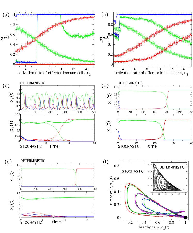
Figure 4: Extinction probabilities, $P_{i}^{ext}$, of tumor ($i=1$, red), healthy ($i=2$, green), and effector immune ($i=3$, blue) cells at increasing activation rates of the immune cells (parameter $r_{3}$), fixing all other model parameters following Itik2010 . (a) Extinction probabilities for the deterministic dynamics (solid triangles), and for the stochastic dynamics using $\sigma_{1,3}=0.1>\sigma_{2}=0$ (open circles). (b) Extinction probabilities using $\sigma_{1,3}=0.05$ (open circles) and $\sigma_{1,3}=0.01$ (solid circles), both also with $\sigma_{2}=0$. Each data point is the mean ($\pm SD)$ computed over $10$ replicas. Each of these replicas was obtained computing the extinction probability for each variable over $200$ time series of length $t=10^{4}$, starting from random low initial conditions for effector and tumor cells, $x_{1,3}(0)<x_{2}(0)=1$ (see Section 4). In the lower panels we display the deterministic and stochastic dynamics for different values of $r_{3}$, with: $r_{3}=3.7$ (c); $r_{3}=9$ (d); and $r_{3}=12.5$. For the stochastic dynamics we display two different runs represented with thin and thick trajectories for each variable, with: (c) $\sigma_{1,3}=0.1$; (d) $\sigma_{1,3}=0.01$; and (e) $\sigma_{1,3}=0.05$, all with $\sigma_{2}=0$. (f) Dynamics projected in the phase space $(x_{2},x_{1})$ using $r_{3}=4$. We display $10$ stochastic trajectories using $\sigma_{1,3}=0.05$. The inset in (f) displays the chaotic attractor for the same initial conditions and parameter values with $\sigma_{1...3=0}$ (i.e., deterministic dynamics).

Using the homotopy solutions, we compute the extinction probabilities, $P_{i=1,2,3}^{ext}$, for each of the cell populations at increasing values of activation rates of effector immune cells, $r_{3}$. The extinction probabilities are computed as follows: for each value of $r_{3}$ analyzed, we built $200$ different time series with the homotopy solutions using $t=10^{4}$. Over these $200$ time series, we calculated the number of time series for each variable fulfilling the extinction condition of variable $i$, assumed to occur when $x_{i}(t)\leq 10^{-30}$, normalizing the number of extinction events over $200$. Then, we repeated the same process $10$ times (replicas), and we computed the mean $(\pm SD)$ of the normalized extinction events over these $10$ replicas. Following the previous procedure, we consider random initial conditions for tumor and effector cells, setting $x_{2}(0)=1$ and $x_{1,3}(0)<x_{2}(0)$, instead of using a single initial condition for each variable for all time series. Specifically, we will consider random initial populations of tumor and effector cells following a uniform distribution within the range $(0,0.2]$. The results are displayed in Fig. 4 using parameter values from Itik2010 , except for the tuned parameter $r_{3}$. The deterministic simulations (solid triangles in Fig. 4a) reveal that extinction probabilities for tumor cells is zero within the range analyzed i.e., $2.4\leq r_{3}\leq 15.5$. For low values of $r_{3}$, the extinction probabilities for healthy and effector cells remain close and low ($P_{2,3}^{ext}\sim 0.05$). Beyond $r_{3}\gtrsim 6$, $P_{2,3}^{ext}$ drastically increases and extinctions take place with probability $1$. Such extinction value is maintained for effector cells at increasing $r_{3}$. The extinction probability of healthy cells diminishes beyond $r_{3}\gtrsim 9.8$ to $P_{2}^{ext}\sim 0.6$. Counterintuitively, these results indicate that increasing activation of effector immune cells (using the parameter values from Itik2010 ) does not involve tumor cells extinction or low extinction probabilities for healthy cells, due to the complexity of the dynamics in the chaotic or fluctuating regimes.

Now, we focus on the effect of demographic stochasticity in the overall dynamics of the system. Figure 4a displays the same analyses performed with the deterministic approach, but now using $\sigma_{1,3}=0.1$ (recall $\sigma_{2}=0$). The observed extinctions patterns drastically change. For instance, the extinction probability of tumor cells, $P_{1}^{ext}$, ranges from $P_{1}^{ext}\sim 0.3$ to $P_{1}^{ext}\sim 0.97$ within the range $2.4\leq r_{3}\leq 15.5$. Moreover, the extinction probability of healthy cells significantly decreases at increasing $r_{3}$, having values of $P_{1}^{ext}\sim 0.05$ for $r_{3}\gtrsim 12.2$. These results clearly indicate that when demographic noise is high (e.g., at initial tumor progression stages) stochastic fluctuations can involve increasing extinction probabilities of tumor cells and increasing survival probabilities of healthy cells when $r_{3}$ grows. In the stochastic simulations, effector immune cells always reached extinction, except for the cases with small $r_{3}$ and low noise amplitudes (Fig. 3b). Similar results were obtained by using $\sigma_{1,3}=0.05$ (open circles in Fig. 4b) and $\sigma_{1,3}=0.01$ (solid circles in Fig. 4b). As expected, the decrease of the noise levels involves lower extinction probabilities for both tumor and healthy cells, although the same tendencies are preserved i.e., increasing $r_{3}$ enlarges tumor cells extinctions and decreases host cells extinctions.

Figure 4(c-d) displays several time series for different values of $r_{3}$ and noise intensities, also representing the deterministic dynamics. For instance, in Fig. 4c (setting $r_{3}=3.7$) the deterministic dynamics is chaotic and no extinctions are found. However, the stochastic dynamics (here using $\sigma_{1,3}=0.1$) can cause extinction or survival of tumor and healthy cells also with $r_{3}=3.7$. In Fig. 4d we use $r_{3}=9$. The deterministic dynamics for this case involves outcompetition of healthy and effector cells by tumor cells. However, the stochastic dynamics ($\sigma_{1,3}=0.01$) can involve either the extinction or survival of tumor cells. Finally, Fig. 4e displays the dynamics using $r_{3}=12.5$. For this case, the deterministic dynamics also involves dominance of tumor cells, but the stochastic dynamics (with $\sigma_{1,3}=0.05$) involves an extinction probability of tumor cells of $P_{1}^{ext}\sim 0.8$. In Fig. 4f we display the trajectories projected in the phase space $(x_{2}(t),x_{1}(t))$ using $r_{3}=4$ and $\sigma_{1,3}=0.05$. The main plot shows ten stochastic trajectories that reach the $(0,1,0)$ attractor (solid black circle) that involves the survival of healthy cells and the extinction of both effector and tumor cells. The inset displays the deterministic dynamics also for $r_{3}=4$, which is governed by the chaotic attractor.

Finally, we want to note that the same qualitative extinction patterns were obtained using parameter values explored in Duarte2013 , setting: $a_{31}=0.9435$ and $a_{13}=5$. Moreover, all the previous simulations (using parameter values from Refs. Itik2010 and Duarte2013 ) were repeated using different extinction thresholds i.e., $x_{i}(t)\leq 10^{-10}$ and $x_{i}(t)\leq 10^{-20}$, and the extinction probabilities remained qualitatively equal for both deterministic and stochastic dynamics (results not shown).

V Discussion

In this article, a semi-analytic method to find approximate solutions for nonlinear differential equations - the step homotopy analysis method (SHAM) - is applied to solve a cancer nonlinear model initially proposed by Itik and Banks Itik2010 . With this algorithm, based on a modification of the homotopy analysis method (HAM) proposed by Liao Liao1992 ; Liao2003 ; Liao2007 , three coupled nonlinear differential equations are replaced by an infinite number of linear subproblems. This modified method has the advantage of giving continuous solutions within each time interval, which is not possible by purely numerical techniques. Associated to the explicit series solutions there is an auxiliary parameter, called convergence-control parameter, that represents a convenient way of controlling the convergence of approximation series, which is a critical qualitative difference in the analysis between HAM/SHAM and other methods.

The model by Itik and Banks Itik2010 considers the dynamics of three interacting cell types: healthy cells, tumor cells, and effector immune cells (i.e., CD8 T cells, also named cytotoxic lymphocytes, CTLs). Our analytical results are found to be in excellent agreement with the numerical simulations. To the best of our knowledge, such kind of explicit series solutions, corresponding to each of the dynamical variables, have never been reported for the Itik-Banks cancer model. The results presented in this article suggest that SHAM is readily applicable to more complex chaotic systems such as Volterra-Lotka type models applied to cancer dynamics. In this work we used the homotopy solutions to investigate the impact of a key parameter in the dynamics of tumor growth: the activation of effector immune cells due to recognition of tumor antigens (parameter $r_{3}$). Previous research has focused on other key parameters of the model by Itik and Banks. For instance, the active suppression of the immune response by the tumor cells has been recently explored in Ref. Duarte2013 . Interestingly, the dynamics were shown to be very sensitive to the suppression of the immune cells, involving an inverse period-doubling bifurcation scenario at increasing the suppression rate of immune cells Duarte2013 . For this case, strong chaos and low predictability was found at small suppression rates, and the chaotic dynamics became more predictable at increasing suppression values. The selective shutdown of the antitumor immune response can also be achieved by the escape of the recognition of the cancer cells by the immune system by selection of non-immunogenic tumor cell variants and in influencing immune cells with a negative regulatory function, such as regulatory T cells and myeloid-derived suppressor cells Thus, the cell-killing activity of the cytotoxic CD8 T cells can be inhibited by the presence within the tumor tissue of immunosuppressive CD4+ regulatory T cells ($T_{reg}$ cells). The function of the $T_{reg}$s is essential for inducing tolerance to ”self ” antigens, preventing autoimmune reactions and for the downregulation of the immune response after the elimination of the antigenic source (such as pathogens, allogenic cells or cancer cells). However, their capacity to inhibit the innate and adaptive anti-tumor immune response also constitute a major obstacle to cancer immunotherapy.

We have used the homotopy solutions to characterize changes in the dynamics at increasing activation rates of the immune cells. Such a parameter is especially important since several clinical therapies are currently available to boost immune responses (see next paragraph). The increase of the immune cells activation rate is shown to cause a period-doubling bifurcation scenario that makes the system to enter into chaotic dynamics. Interestingly, the populations of tumor cells, although undergoing large fluctuations, are able to survive for all the range of $r_{3}$ analyzed. In order to simulate demographic stochasticity that might be found at early stages of tumorigenesis, we added noise terms to the homotopy solutions for tumor and effector immune cells populations. As a difference from the deterministic dynamics, we found that an increase of $r_{3}$ increases the extinction probabilities for tumor cells, also diminishing the extinction probabilities of healthy cells. These results suggest that possible therapies enhancing the activation of effector immune cells (see next paragraph) at early stages of tumor progression could result in higher probabilities of stochastic tumor clearance. lt is worth to note that the model proposed by Itik and Banks does not explicitly model the clonal expansion of immune cells after tumor antigen recognition that could make the noise in CTLs populations to be even smaller or negligible. It is known that after being activated, the population of CTLs is expanded in order to exert strong cytotoxic effects. Then, the CD8 response is downregulated by programmed cell death mechanisms to avoid over-activation of the immune system (Raval et al., 2014). Due to the complexity of the dynamics found at increasing $r_{3}$, it is not clear if clonal expansion would favor the extinction of tumor cells, as we would expect. In this sense, the effect of immune system activation together with production of large populations of effector immune cells due to clonal expansion (burst in the population of effector immune cells) should be modeled to determine if our observed results remain the same or change the probabilities of tumor cells extinction in response to increases in $r_{3}$.

Our results could be clinically relevant since several therapies to stimulate and activate immune cells are currently available. A foundational property of the immune system is its capacity to distinguish between the ”self ” and ”non-self ” antigens. In the context of an evolving tumor, it is likely that the tumoral cells will present to the immune cells a number of new antigens product of the genetic aberrations present in their genome. This mechanism is probably involved in the control of early tumors. However, it is known that cancer cells escape innate and adaptive immune responses by selection of non-immunogenic tumor cell variants (immunoediting) or by active suppression of the immune response (immunosubversion) (see Raval2014 for a review). Tumor antigens often elicit poor adaptive immune responses because they are recognized as ”self-antigens” that induce tolerance, the natural mechanism of the body to prevent autoimmunity. The enhancement of the antitumor T cell responses by triggering TCR costimulatory molecules to break tolerance has been envisaged as a way to potentiate the antitumor immune functions. Agonists of the costimulatory tumor necrosis factor receptor (TNFR) family members, which include proteins involved in B and T cell development, survival, and immune activation, have been proven to enhance the antitumor immune responses. Preclinical and early clinical data of the use of agonists of 4-1BB (CD137) or OX40 (CD134) support further studies of these costimulatory molecules as potentiators of the antitumor response Schaer2014 . An increasingly successful anticancer strategy that aims to boost immune responses against tumor cells consists in enhancing the cell-killing activity of the cytotoxic CD8 T cells by the use of antibodies that block negative regulators of T-cell activation (”checkpoint inhibitors”). Fully humanized monoclonal antibodies blocking the inhibitory molecules Cytotoxic T-Lymphocyte antigen 4 (CTLL4, Ipilimumab, Tremelimumab) or Programmed Death Receptor-1 (PD-1, Nivolumab, MK-3475) have been proven to be useful in solid tumors such as melanoma, renal cell carcinoma, non small cell lung cancer or colorectal cancer (reviewed in Kyi2014 ). More recently, the p110$\delta$ isoform of phosphoinositide-3-OH kinase (PI(3)K) activity has been shown to be required for the proliferation and differentiation of suppressive $T_{reg}$ cells induced by tumor cells. PI(3)K $\delta$ inhibitors have been proven to be able to preferentially inhibit CD4 $T_{reg}$ cells over effector CTLs, opening new ways to unleash the power of dormant anti-tumor immune cells Ali2014 . More recent and novel approaches suggest the possibility to increase CTLs activation by means of artificial APCs (see Eggermont2014 for further details).

Summarizing, our results suggest that potential therapies increasing activation rates of effector immune cells might be much more effective at early stages of tumor progression, when demographic noise becomes important in tumor cells populations. Our results also suggest that the stimulation of immune cells may not facilitate tumor clearance in cancers with large population numbers of tumor cells, as the deterministic approach is considering. Further research should also analyze the robustness and generality of our results to changes in the other model parameters. As discussed in Duarte2013 , it would be also interesting to explore the effect of increasing the activation of effector immune cells in solid tumors by means of a spatial version of the cancer model analyzed in this article.

- (1) Lyapunov, A.M.: General problem on stability of motion. Taylor & Francis, London (1992)
- (2) Karmishin, A.V., Zhukov, A.T., Kolosov, V.G.: Methods of dynamics calculations and testing for thin-walled structures. Moscow: Mashinostroyenie (1990)
- (3) Awrejcewicz, J., Andrianoc, I.V., Manevitch, L.I.: Asymtotic approaches in nonlinear dynamics. Springer-Verlag, Berlin (1998)
- (4) Adomian, G.: Nonlinear stochastic differential equations. J. Math. Appl. 55, 441-452 (1976)
- (5) Adomian, G.: A review of the decomposition method and some recent results for nonlinear equations. Comp. and Math. Appl. 21, 101-127 (1991)
- (6) Rach, R.: On the Adomian method and comparisons with Picard’s method. J. Math. Appl. 10, 139-159 (1984)
- (7) Adomian, G., Adomian G.E.: A global method for solution of complex systems. Math. Model. 5, 521-568 (1984)
- (8) Liao, S.J.: The proposed homotopy analysis techniques for the solution of nonlinear problems. Ph.D. dissertation. Shanghai: Shanghai Jiao Tong University (1992)
- (9) Liao, S.J.: Beyond perturbation: introduction to the homotopy analysis method. CRC Press, Boca Raton, Chapman and Hall (2003)
- (10) Sen, S.: Topology and geometry for physicists. Florida: Academic Press (1983)
- (11) Liao, S.J., Tan, Y. A general approach to obtain series solutions of nonlinear differential equations. Stud. Appl. Math. 119, 297-355 (2007)
- (12) Alomari, A.K., Noorani, M.S.M., Nazar, R., Li, C.P.:Homotopy analysis method for solving fractional Lorenz system. Commun. Nonlinear Sci. Numer. Simulat. 15, 1864-1872 (2010)
- (13) Hayat, T., Khan, M. Homotopy solutions for a generalized second-grade fluid past a porous plate. Nonlinear Dyn. 42, 395-405 (2005)
- (14) Li, H., Guo, Y.: New exact solutions to the Fitzhugh-Nagumo equation. Appl. Math. Comp. 180, 524-528(2006)
- (15) Abbasbandy, S.: Soliton solutions for the Fitzhugh-Nagumo equation with the homotopy analysis method. Appl. Math. Model. 32, 2706-2714 (2008)
- (16) Arafa, A.M.M., Rida, S. Z., Mohamed, H.: Homotopy analysis method for solving biological population model. Commun. Theor. Phys. 56, 797-800 (2011)
- (17) Putcha, V.S. Two Species and Three Species Ecological Modeling - Homotopy Analysis, Diversity of Ecosystems, Prof. Mahamane Ali (Ed.), ISBN: 978-953-51-0572-5, InTech, DOI: 10.5772/37146 (2012)
- (18) Khan, H., Mohapatra, R.N., Vajravelu, K., Liao, S.J.: The explicit series solution of SIR and SIS epidemic models. Appl. Math. and Comp. 215, 653-669 (2009)
- (19) Usha, S., Abinaya, V., Loghambal, S., Rajendran, L. Non-linear mathematical model of the interaction between tumor and oncolytic viruses. Appl. Math. 3, 1-8 (2012)
- (20) Itik, M., Banks, S. P.: Chaos in a three-dimensional cancer model. Internat. J. Bifurc. Chaos 20, 71-79 (2010)
- (21) Hastings, A., Powell, T.: Chaos in a three-species food chain. Ecology 72(3), 896-903 (1991)
- (22) Vano, J.A, Wildenberg, J. C., Anderson, M.B., Nodel, J. K., Sprott, J. C.: Chaos in low-dimensional Lotka-Volterra models of competition. Nonlinearity 19, 2391-2404 (2006)
- (23) Gakkhar, S., Naji, R.K.: Existence of chaos in two-prey, one-predator system. Chaos Solit. Fract. 17, 639-649.
- (24) Tang, S., Chen, L.: Chaos in functional response host-parasitoid ecosystem models. Chaos Solit. Fract. 13, 875-884 (2002)
- (25) Kuznetsov, V. A., Makalkin, I. A., Taylor, M. A. Perelson, A. S. Nonlinear dynamics of immunogenic tumors: Parameter estimation and global bifurcation analysis,. Bull. Math. Biol. 56, 295-321 (1994)
- (26) de Pillis, L. G., Radunskaya, A.: The dynamics of an optimally controlled tumor model: A case study. Math. Comput. Model. 37, 1221-1244 (2003)
- (27) Kirschner, D., Panetta, J. C. Modeling immunotherapy of the tumor-immune interaction, J. Math. Biol. 37, 235-252 (1998)
- (28) Letellier, C., Denis, F., Aguirre, L. A. What can be learned from a chaotic cancer model? J. Theor. Biol. 322, 7-16 (2013)
- (29) Duarte, J., Januario, C., Rodrigues, C., Sardanyés, J.: Topological complexity and predictability in the dynamics of a tumour growth model with Shilnikov’s Chaos. Int. J. Bifurc. Chaos 23, 1350124 (2013)
- (30) López, A.G., Sabuco, J., Seoane, J.M., Duarte, J., Januário, C., Sanjuán, M-A.S.: Avoiding healthy cells extinction in a cancer model. J. Theor. Biol. 349, 74-81 (2014)
- (31) Denis, F., Letellier, C.: Chaos theory: a fascinating concept for oncologists. Cancer Radiotherapy 16, 230-235 (2012)
- (32) Denis, F., Letellier, C.: Radiotherapy and chaos therapy: the tit and the butterfly. Cancer Radiotherapy 16, 404-409 (2012)
- (33) Kuznetsov, V. A., Knott, G. D.: Modeling tumor regrowth and immunotherapy. Math. Comput. Model. 33, 1275-1287 (2001)
- (34) de Pillis, L. G., Gu, W.,Radunskaya, A. E. Mixed immunotherapy and chemotherapy of tumors: Modeling, applications and biological interpretations. J. Theoret. Biol. 238, 841-862 (2006)
- (35) Itik, M., Salamci, M. U., Banks, S. P. Optimal control of drug therapy in cancer treatment. Nonlin. Anal. Th. Meth. Appl. 71, e1473-e1486 (2009)
- (36) Bajzer, Z., Marusic, M., Vuk-Pavlovic, S. Conceptual frameworks for mathematical modeling of tumor growth dynamics. Math. Comput. Model. 23, 31-46 (1996).
- (37) Chua, L.O., Parker, T.S. Practical Numerical Algorithms for Chaotic Systems (Springer-Verlag New York Inc.), New York (1989)
- (38) Berryman, A.A., Millstein, J.A.: Are ecological systems chaotic - And if not, why not? Trends Ecol. Evol. 4(1), 26-28 (1989)
- (39) Allen, J.C., Schaffer, W. M., Rosko, D. Chaos reduces species extinction by amplifying local population noise. Nature 364, 229-232 (1993)
- (40) Sardanyés, J. Low-dimensional homeochaos in coevolving host-parasitoid dimorphic populations: Extinction thresholds under local noise. Comm. Nonlin. Sci. Numer. Simula 16, 3896-3903 (2011)
- (41) Raval, R.R., Sharabi, A.B., Walker, A.J., Drake. C.G., Sharma, P.: Tumor immunology and cancer immunotherapy: summary of the 2013 SITC primer. J. Immunother Cancer, textbf2:14 (2014)
- (42) Kyi, C., Postow, M.A.: Checkpoint blocking antibodies in cancer immunotherapy. FEBS Lett., 588:368-376 (2014)
- (43) Schaer, D.A., Hirschhorn-Cymerman, D., Wolchok, J.D. Targeting tumor-necrosis factor receptor pathways for tumor immunotherapy. J Immunother Cancer 2:7 (2014)
- (44) Ali, K., Soond, D.R., Pi eiro, R., Hagemann, T., Pearce, W., Lim, E.L., Bouabe, H., Scudamore, C.L., Hancox, T., Maecker, H., Friedman, L., Turner, M., Okkenhaug, K., Vanhaesebroeck, B. Inactivation of PI(3)K p110? breaks regulatory T-cell-mediated immune tolerance to cancer. Nature, 509:407-411 (2014)
- (45) Eggermont, L.J., Paulis, L.E., Tel, J., Figdor, C.G. Toward efficient cancer immunotherapy: advances in developing artificial antigen-presenting cells. Trends in Biotechnology. In Press (2014)