Higgs Phenomenology of the Supersymmetric Grand Unification with the Hosotani Mechanism

Abstract

The supersymmetric $SU(5)$ grand unified theory with the gauge symmetry broken by the Hosotani mechanism naturally solves the mass hierarchy problem between the colored Higgs triplet and the electroweak Higgs doublet, and predicts the existence of adjoint chiral superfields with masses of the order of the supersymmetry breaking scale as a byproduct. In addition to the two $SU(2)_{L}$ Higgs doublets of the minimal supersymmetric standard model, the Higgs sector is extended by an $SU(2)_{L}$ triplet chiral supermultiplet with hypercharge zero and a neutral singlet one. Such new triplet and singlet chiral supermultiplets deviate the standard model-like Higgs boson couplings and the additional Higgs boson masses from their Standard Model predictions. We show that this model can be distinguished from other new physics models using by precisely measuring such Higgs couplings and masses, and that our model is a good example of grand unification testable at the luminosity up-graded Large Hadron Collider and future electron-positron colliders.

1 Introduction

One of the most significant development in the past decades is the discovery of a new particle with mass of approximately 125 GeV, which was announced by the ATLAS and CMS collaborations at the CERN Large Hadron Collider (LHC) in 2012 [2]. The spin and CP properties as well as the couplings have been analyzed, and it has been shown that the nature of the discovered particle is consistent with the Standard Model (SM) Higgs boson. Therefore, the SM is established as a low energy effective theory that consistently explains phenomena below the TeV scale.

However, the SM have problems that should be resolved in a more fundamental theory. Since the SM Higgs boson is an elementary scalar, an unnatural cancellation between its bare mass squared and quadratically divergent contributions from radiative corrections is required. in order to keep the Higgs boson mass to the weak scale. The reason for the fact that the electric charges of the SM particles are fractionally quantized is not explained.

It is intriguing that that the above-mentioned problems can be solved by introducing the concepts of supersymmetry (SUSY) and grand unification [3, 4]. In supersymmetric extensions of the SM, the loop contributions from SM particles are canceled with those from superpartners, and the problem of the quadratic divergence in the Higgs boson mass squared is avoided. In Grand Unified Theories (GUTs), the SM gauge groups is embedded into a larger gauge group. Simultaneously, the SM fermions are also embedded into larger representations. If the GUT gauge group is (semi-)simple, quantization of the electric charges of the SM particles is automatically realised. Therefore, models of SUSY GUTs are excellent candidates for physics beyond the SM.

However, there are have several unattractive points in SUSY GUTs. It should be noticed that the typical energy scale where the three SM gauge couplings are unified is around $10^{16}$ GeV in ordinary SUSY GUTs. Due to the decoupling theorem, the effects of the GUT-scale particles are negligible at the TeV scale [5]. Remnants of physics realized at the GUT scale can be investigated only through relations among the masses and couplings of TeV-scale particles. Although the colored Higgs triplets and the electroweak Higgs doublets originate from the same multiplets, an unnaturally huge mass splitting between them are supposed for suppressing proton decay. To address this this doublet-triplet splitting problem many ideas have been proposed [6, 7, 8, 9, 10, 11].

On the contrary, in the model where the doublet-triplet mass splitting is realized by supersymmetrizing the Grand Gauge-Higgs Unification (GHU) model, the existence of new light particles whose masses are of the order of the TeV scale is predicted [12]. The Grand Gauge-Higgs Unification is constructed on an extra dimension whose compactification scale is around the GUT scale [13], and the GUT gauge symmetry is broken due to the Hosotani mechanism [14]: The non-trivial vacuum expectation value (VEV) of the extra-dimensional component of one of the gauge fields accounts for the GUT symmetry breaking.

In the Supersymmetric Grand Gauge-Higgs Unification (SGGHU) model, there appear a color octet chiral superfield, an $SU(2)_{L}$ triplet chiral superfield with hypercharge zero and a neutral singlet chiral superfield at the TeV scale as a by-product. As compared to the Minimal Supersymmetric Standard Model (MSSM), the Higgs sector is extended with the triplet and singlet chiral superfields.

In this presentation, we focus on the properties of the Higgs sector of the SGGHU model, and discuss its phenomenological signatures expected at collider experiments. The masses and couplings of the SGGHU Higgs sector particles are determined by solving renormalization group equations (RGEs) from the GUT scale to the electroweak scale. We emphasize that models beyond the SM can be distinguished by precisely measuring the masses and couplings of the Higgs bosons at the LHC and future electron-positron colliders such as the International Linear Collider (ILC) [15] and the CLIC [16]. The SGGHU　model is a good example to show that collider experiments are capable of testing GUT-scale physics.

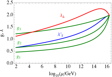
Figure 1: RG evolution of the Higgs triplet and singlet couplings $\lambda_{\Delta}$ (red line) and $\lambda^{\prime}_{S}$ (blue) as well as the gauge couplings $g_{3}$, $g_{2}$ and $g_{1}$ (green) at the one loop level as a function of the energy scale $\mu$.

2 Supersymmetric Grand Gauge-Higgs Unification

Let us discuss the Higgs sector of the low energy effective theory of the SGGHU model. At the TeV scale, the SGGHU Higgs sector consists of an $SU(2)_{L}$ triplet chiral superfield $\Delta$ and an neutral singlet chiral superfield $S$ as well as the two MSSM Higgs doublets $H_{u}$ and $H_{d}$. The superpotential is given by

$$W = \mu H_{u}\cdot H_{d}+\mu_{\Delta}{\rm tr}(\Delta^{2})+\frac{\mu_{S}}{2}S^{2}$$ (1)

$$+\lambda_{\Delta}H_{u}\cdot\Delta H_{d}+\lambda_{S}SH_{u}\cdot H_{d}\,,$$

where $\Delta=\Delta^{a}\sigma^{a}/2$ with $\sigma^{a}$ $(a=1,2,3)$ being the Pauli matrices. Since the triplet $\Delta$ and singlet $S$ originate from the gauge supermultiplet, the following remarkable features are predicted. Trilinear self-couplings among $S$ and $\Delta$ vanish although they are not prohibited in the general Higgs superpotential with the triplet and singlet superfields. The Higgs couplings $\lambda_{\Delta}$ and $\lambda_{S}$ are unified with the SM gauge couplings at the GUT scale. Therefore, the properties of the Higgs bosons are predicted with less ambiguity. The soft SUSY breaking operators in the Higgs potential are given by

$$V_{\rm soft} = \widetilde{m}_{H_{d}}^{2}|H_{d}|^{2}+\widetilde{m}_{H_{u}}^{2}|H_{u}|^{2}$$ (2)

$$+2\widetilde{m}_{\Delta}^{2}{\rm tr}(\Delta^{\dagger}\Delta)+\widetilde{m}_{S}^{2}|S|^{2}$$

$$+\left[B\mu H_{u}\cdot H_{d}+\xi S+B_{\Delta}\mu_{\Delta}{\rm tr}(\Delta^{2})\right.$$

$$+\frac{1}{2}B_{S}\mu_{S}S^{2}+\lambda_{\Delta}A_{\Delta}H_{u}\cdot\Delta H_{d}$$

$$\left.+\lambda_{S}A_{S}SH_{u}\cdot H_{d}+{\rm h.c.}\right].$$

The soft parameters at the TeV scale are computed by solving the RGEs. After radiative electroweak symmetry breaking, four CP-even, three CP-odd and three charged Higgs bosons appear as physical particles. The VEV of the neutral component of the triplet Higgs boson $v_{\Delta}$, which is derived from the minimization conditions of the Higgs potential, must be less than $\simeq 10~{}{\rm GeV}$ in order to be consistent with the rho parameter constraint. Since $v_{\Delta}$ is sufficiently small compared to $v=246~{}{\rm GeV}$, it is negligible in the computations of the Higgs boson masses and couplings.

3 Analysis of the Renormalization Group Equations

Here, we discuss RG evolution of couplings and masses in the SGGHU model. The introduction of the light adjoint multiplets disturbs the successful gauge coupling unification. One can easily recover the gauge coupling unification by adding extra incomplete $SU(5)$ matter multiplets. A judicious choice for the matter multiplets is a set of two vectorlike pairs of $(\bar{L},L)$ $(({\bf 1},{\bf 2})_{-1/2})$, one of $(\bar{U},U)$ $((\bar{\bf 3},{\bf 1})_{-2/3})$ and one of $(\bar{E},E)$ $(({\bf 1},{\bf 1})_{1})$. Here, the numbers in the parentheses denote $SU(3)_{C}$, $SU(2)_{L}$ and $U(1)_{Y}$ quantum numbers, respectively [12]. Fig. 1 shows the RG evolution of the Higgs triplet and singlet couplings $\lambda_{\Delta}$ (red line) and $\lambda_{S}$ (blue) as well as the gauge couplings $g_{3}$ , $g_{2}$ and $g_{1}$ (green) at the one loop level as a function of the energy scale $\mu$. The couplings are normalized such that $\lambda^{\prime}_{S}=(2\sqrt{5/3})\lambda_{S}$ for the singlet Higgs coupling and $g_{1}=(\sqrt{5/3})g_{Y}$ for the $U(1)_{Y}$ gauge coupling. The resulting Higgs trilinear couplings at the TeV-scale are given by

$$\lambda_{\Delta}=1.1\,,\qquad\lambda_{S}=0.25\,.$$ (3)

The soft SUSY breaking parameters at the TeV scale are also derived by solving the RGEs. As shown in Fig. 1, the gauge couplings become strong around the GUT scale. Since the unified gaugino mass at the GUT scale has to be large in order to avoid the gluino mass bound [17], typical values for the soft sfermion and Higgs masses at the SUSY breaking scale are in the multi-TeV range. Therefore, some tuning is needed for successful radiative electroweak symmetry breaking. In spite of such difficulties, we can also obtain soft Higgs mass parameters of the order of ${\cal O}(100)$ GeV by tuning among the input parameters at the GUT scale, as shown in the next section.

4 Impact on the Properties of the Higgs Sector

The prediction about the SM-like Higgs boson mass is affected by its interactions with the $SU(2)_{L}$ triplet and singlet Higgs multiplets. When the soft scalar masses of the triplet and singlet Higgs multiplets are relatively large, the approximate formula for the SM-like Higgs boson mass is [18, 19]

$$m_{h}^{2} \simeq m_{Z}^{2}\cos^{2}\beta$$ (4)

$$+\frac{3m_{t}^{4}}{2\pi^{2}v^{2}}\left(\ln{\frac{m_{\tilde{t}}^{2}}{m_{t}^{2}}}+\frac{X_{t}^{2}}{m_{\tilde{t}}^{2}}\left(1-\frac{X_{t}^{2}}{12m_{\tilde{t}}^{2}}\right)\right)$$

$$+\frac{1}{8}\lambda_{\Delta}^{2}v^{2}\sin^{2}{2\beta}+\frac{1}{2}\lambda_{S}^{2}v^{2}\sin^{2}{2\beta}\,,$$

where $m_{Z}$ is the $Z$-boson mass, $m_{t}$ is the top quark mass, $m_{\tilde{t}}$ is the geometrical average of the stop mass eigenvalues, and $X_{t}=A_{t}-\mu\cot\beta$. In the MSSM, large stop masses are required even in the maximal stop mixing case in order to obtain an SM-like Higgs boson mass of 125 GeV [20]. In our model, on the contrary, the SM-like Higgs boson mass is lifted up by the Higgs trilinear interactions with the triplet and singlet superfields for small $\tan\beta$. Notice that the same mechanism is realized in the next-to-MSSM (NMSSM) [21]. For our numerical computations of the masses of the Higgs bosons and their superpartners, we have appropriately modified the public numerical code SuSpect [22] by adding the contributions from the triplet and singlet Higgs superfields. Since some fine tuning for the GUT-scale input parameters is needed, we show our numerical results based on several benchmark points that can reproduce the observed SM-like Higgs boson mass. Because of theoretical uncertainties in the computation of the SM-like Higgs boson mass, we take $122~{}{\rm GeV}<m_{h}<129~{}{\rm GeV}$ as its allowed mass range. We focus on the following three typical cases:

• Mixings between the SM-like Higgs boson and the other CP-even Higgs bosons are small.

• Mixings between the SM-like Higgs bosons and the CP-even components of the triplet and singlet Higgs fields are small.

• The CP-even components of the triplet and singlet Higgs fields affect the SM-like Higgs boson couplings.

Three successful benchmark points for the GUT-scale input parameters and the TeV-scale parameters obtained after solving the RGEs are listed in Tab. 1 and 2, respectively.

Case	$\tan\beta$	$M_{1/2}$	$\mu_{\Sigma}$
(A)(B)(C)	$3$	$3600~{}{\rm GeV}$	$-300~{}{\rm GeV}$

Case	$A_{0}$	$\widetilde{m}_{0}^{2}$	$\widetilde{m}_{H_{u}}^{2}$	$\widetilde{m}_{H_{d}}^{2}$	$\widetilde{m}_{5}^{2}$	$\widetilde{m}_{10}^{2}$	$\widetilde{m}_{\Sigma}^{2}$
(A)	$5500~{}{\rm GeV}$	$(1000~{}{\rm GeV})^{2}$	$(10375~{}{\rm GeV})^{2}$	$(8570~{}{\rm GeV})^{2}$	$-(6300~{}{\rm GeV})^{2}$	$-(2000~{}{\rm GeV})^{2}$	$-(570~{}{\rm GeV})^{2}$
(B)	$1000~{}{\rm GeV}$	$(1800~{}{\rm GeV})^{2}$	$(12604~{}{\rm GeV})^{2}$	$(10381.5~{}{\rm GeV})^{2}$	$-(7700~{}{\rm GeV})^{2}$	$-(1960~{}{\rm GeV})^{2}$	$-(670~{}{\rm GeV})^{2}$
(C)	$8000~{}{\rm GeV}$	$(3000~{}{\rm GeV})^{2}$	$(10605.1~{}{\rm GeV})^{2}$	$(8751.4~{}{\rm GeV})^{2}$	$-(6418~{}{\rm GeV})^{2}$	$-(1638.5~{}{\rm GeV})^{2}$	$-(400~{}{\rm GeV})^{2}$

Table 1: Benchmark points for the input parameters at the GUT scale.

Case	$M_{1}$	$M_{2}$	$M_{3}$	$\mu_{\Delta}$	$\mu_{S}$
(A)(B)(C)	$194~{}{\rm GeV}$	$388~{}{\rm GeV}$	$1360~{}{\rm GeV}$	$-252~{}{\rm GeV}$	$-85.8~{}{\rm GeV}$

Case	$\mu$	$B\mu$	$\widetilde{m}_{u_{3}}$	$\widetilde{m}_{q_{3}}$	$y_{t}A_{t}$
(A)	$205~{}{\rm GeV}$	$41400~{}{\rm GeV}^{2}$	$3290~{}{\rm GeV}$	$4830~{}{\rm GeV}$	$4030~{}{\rm GeV}$
(B)	$177~{}{\rm GeV}$	$40800~{}{\rm GeV}^{2}$	$1730~{}{\rm GeV}$	$4480~{}{\rm GeV}$	$6050~{}{\rm GeV}$
(C)	$174~{}{\rm GeV}$	$42000~{}{\rm GeV}^{2}$	$4220~{}{\rm GeV}$	$5550~{}{\rm GeV}$	$2910~{}{\rm GeV}$

Case	$\widetilde{m}_{\Delta}$	$\widetilde{m}_{S}$	$\lambda_{\Delta}A_{\Delta}$	$\lambda^{\prime}_{S}A_{S}$	$B_{\Delta}\mu_{\Delta}$	$B_{S}\mu_{S}$	$m_{h}$
(A)	$607~{}{\rm GeV}$	$805~{}{\rm GeV}$	$662~{}{\rm GeV}$	$683~{}{\rm GeV}$	$92000~{}{\rm GeV}^{2}$	$-78700~{}{\rm GeV}^{2}$	$123~{}{\rm GeV}$
(B)	$784~{}{\rm GeV}$	$612~{}{\rm GeV}$	$1340~{}{\rm GeV}$	$1110~{}{\rm GeV}$	$30700~{}{\rm GeV}^{2}$	$-110000~{}{\rm GeV}^{2}$	$123~{}{\rm GeV}$
(C)	$521~{}{\rm GeV}$	$216~{}{\rm GeV}$	$284~{}{\rm GeV}$	$446~{}{\rm GeV}$	$207000~{}{\rm GeV}^{2}$	$-33600~{}{\rm GeV}^{2}$	$122~{}{\rm GeV}$

Table 2: TeV-scale parameters obtained by solving the RGEs.

The couplings between the SM-like Higgs boson and SM particles can be significantly altered due to the existence of the triplet and singlet Higgs bosons. In discussing the SM-like Higgs boson couplings, it is useful to introduce the scaling factors defined as

$$\kappa_{X}=\frac{g_{hXX}}{g_{hXX}|_{\rm SM}}\,,$$ (5)

where $g_{hXX}$ is the coupling with the SM particle $X$. Fig. 2 shows the deviations in the scaling factors $\kappa_{X}$ are plotted on the $\kappa_{\tau}$-$\kappa_{b}$ plane, the $\kappa_{V}$-$\kappa_{b}$ plane $(V=Z,W)$ and the $\kappa_{c}$-$\kappa_{b}$ plane. The deviations in the three SGGHU benchmark points (A), (B) and (C) are shown with green blobs. The MSSM predictions are displayed with red lines for $\tan\beta=10$ (thick line) and $\tan\beta=3$ (dashed). The NMSSM predictions are shown with blue grid lines for $\tan\beta=10$ (thick) and $\tan\beta=3$ (dashed), which denote mixings between the SM-like and singlet-like Higgs bosons of 10%, 20% and 30% from the right to the left. Notice that the SM-like Higgs boson couplings to the down-type quarks and charged leptons are common in this model, as in the type-II two-Higgs-doublet model. Therefore, the MSSM, NMSSM and SGGHU predict $\kappa_{b}/\kappa_{\tau}=1$ at the tree level. At the ILC with $\sqrt{s}=500~{}{\rm GeV}$, expected accuracies for the Higgs boson couplings are $\kappa_{Z}$, $\kappa_{W}$, $\kappa_{b}$, $\kappa_{\tau}$ and $\kappa_{c}$ are 1.0% 1.1% 1.6%, 2.3% and 2.8%, respectively [23]. Fig. 2 shows that typical SGGHU predictions about the scaling factors can be distinguished from the corresponding SM and MSSM predictions through precision measurements of the Higgs boson couplings at the future ILC. It may be difficult to completely distinguish our model from the NMSSM only from the Higgs boson couplings. However, if the pattern of the deviations of the Higgs couplings is found to be close to one of our benchmark scenarios, the possibility of the SGGHU is increased. Independent measurement of $\tan\beta$ using Higgs boson decay at the ILC [25, 26] will be also helpful in discriminating TeV-scale models. For the above benchmark points, the predicted range of the Higgs boson coupling with the photon and that of the Higgs self-coupling are $0.94<\kappa_{\gamma}<1.0$ and $0.82<\kappa_{h}<0.93$, respectively. More precise measurements at the ILC with $\sqrt{s}=1~{}{\rm TeV}$ [23] are needed in order to observe such small deviations.

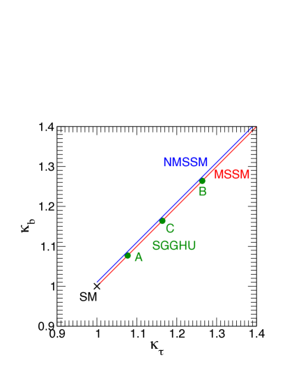
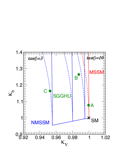
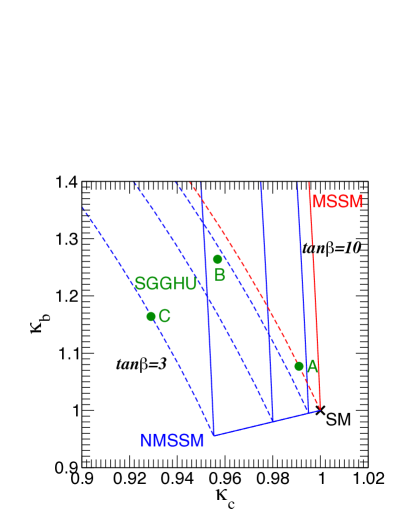
Figure 2: The scaling factors $\kappa_{X}$ are plotted on the $\kappa_{\tau}$-$\kappa_{b}$ plane, the $\kappa_{V}$-$\kappa_{b}$ plane $(V=Z,W)$, and the $\kappa_{c}$-$\kappa_{b}$ plane. The deviations in the three benchmark scenarios (A), (B) and (C) in the SGGHU are shown with green blobs. The MSSM predictions are shown with red lines for $\tan\beta=10$ (thick line) and $\tan\beta=3$ (dashed). The NMSSM predictions are shown with blue grid lines for $\tan\beta=10$ (thick) and $\tan\beta=3$ (dashed), which indicate mixings between the SM-like and singlet-like Higgs bosons of 10%, 20% and 30% from the right to the left.

Let us turn to discussions on the masses of the additional MSSM-like Higgs bosons. Given relatively large soft scalar masses of the Higgs triplet and singlet fields, the approximate formula for the MSSM-like charged Higgs boson mass $m_{H^{\pm}}$ is given by

$$m_{H^{\pm}}^{2} = m_{H^{\pm}}^{2}|_{\rm MSSM}(1+\delta_{H^{\pm}})^{2}$$ (6)

$$\simeq m_{A}^{2}+m_{W}^{2}+\frac{1}{8}\lambda_{\Delta}^{2}v^{2}-\frac{1}{2}\lambda_{S}^{2}v^{2}\,,$$

where $m_{A}$ stands for the MSSM-like CP-odd Higgs boson mass, and $\delta_{H^{\pm}}$ parametrizes the deviation of $m_{H^{\pm}}$ from its MSSM prediction. The sign difference between the triplet and singlet contributions arises from group theoretical factors. Since we have $\lambda_{\Delta}>\lambda_{S}/2$ due to radiative corrections, the MSSM-like charged Higgs boson mass in our model is larger than its MSSM prediction. Fig. 3 shows the mass deviation parameter $\delta_{H^{\pm}}$ as a function of $m_{A}$ for relatively large soft Higgs masses. The black, blue and green lines represent triplet contribution, singlet contribution and their sum, respectively. When the masses of the MSSM-like Higgs bosons are smaller than $500~{}{\rm GeV}$, the deviation parameter is $\delta_{H^{\pm}}\sim O(1)~{}\%$ - $O(10)~{}\%$ and measurable at the LHC [24].

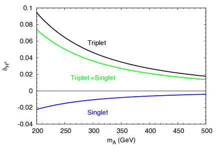
Figure 3: The mass deviation parameter $\delta_{H^{\pm}}$ as a function of the MSSM-like CP-odd Higgs boson mass $m_{A}$ for relatively large soft Higgs masses. The black, blue and green lines represent triplet contribution, singlet contribution and their sum, respectively.

If the masses of the triplet-like and singlet-like Higgs bosons are smaller than $500~{}{\rm GeV}$, these new particles can be directly produced at the ILC and CLIC. As shown in Tab. 3, such light Higgs bosons are realized in the benchmark scenario (C). For instance, $\Delta^{\pm}$ can be probed through the channel $e^{+}e^{-}\to\Delta^{+}\Delta^{-}\to t\bar{b}\bar{t}b$, which is induced by the mixing between the triplet-like and MSSM-like charged Higgs bosons.

CP-even	CP-odd	Charged
$122~{}{\rm GeV}$	$-$	$-$
$139~{}{\rm GeV}$	$171~{}{\rm GeV}$	$204~{}{\rm GeV}$
$370~{}{\rm GeV}$	$304~{}{\rm GeV}$	$496~{}{\rm GeV}$
$745~{}{\rm GeV}$	$497~{}{\rm GeV}$	$745~{}{\rm GeV}$

Table 3: The mass spectrum of the Higgs bosons for the benchmark scenario (C).

As discussed above, comprehensive analysis of the masses and couplings of the Higgs bosons at the LHC and future electron-positron colliders can distinguish models realized at the TeV scale. Even if the additional Higgs bosons are beyond the reach of direct discovery, their effects are left in the SM-like Higgs boson couplings and the MSSM Higgs masses and can be indirectly probed by their precision measurements. Therefore, a new electron-positron collider is mandatory for exploring the Higgs sector and the underlying theory.

5 Summary

In the SUSY $SU(5)$ GUT model where the Hosotani mechanism accounts for the GUT symmetry breaking, the low-energy Higgs sector involves a Higgs triplet and singlet chiral superfields as well as the two MSSM Higgs doublets. We have evaluated the SM-like Higgs boson couplings to SM particles. It is shown that these couplings deviate from the corresponding SM predictions by ${\cal O}(1)\%$ when the triplet and singlet Higgs bosons are lighter than $\simeq 1~{}{\rm TeV}$. Such deviations are measurable at future electron-positron colliders. When the masses of the MSSM-like charged Higgs boson and the MSSM-like CP-odd Higgs boson are less than $\simeq 500~{}{\rm GeV}$, their mass difference is larger than the MSSM prediction by ${\cal O}(1)\%$ - ${\cal O}(10)\%$, and can be measured at the LHC. Using these observations, our model can be distinguished from the MSSM and NMSSM. We emphasise that our supersymmetric grand gauge-Higgs unification model is a good example to show that colliders are able to test physics realized at the GUT scale.

References

- [1] M. Kakizaki, S. Kanemura, H. Taniguchi and T. Yamashita, Phys. Rev. D 89, 075013 (2014).
- [2] G. Aad et al. [ATLAS Collaboration], Phys. Lett. B 716, 1 (2012); S. Chatrchyan et al. [CMS Collaboration], Phys. Lett. B 716, 30 (2012).
- [3] H. Georgi and S. L. Glashow, Phys. Rev. Lett. 32 (1974) 438.
- [4] E. Witten, Nucl. Phys. B 188 (1981) 513; S. Dimopoulos, S. Raby and F. Wilczek, Phys. Rev. D 24 (1981) 1681; S. Dimopoulos and H. Georgi, Nucl. Phys. B 193 (1981) 150; N. Sakai, Z. Phys. C 11 (1981) 153.
- [5] T. Appelquist and J. Carazzone, Phys. Rev. D 11, 2856 (1975).
- [6] S. Dimopoulos and F. Wilczek, NSF-ITP-82-07; M. Srednicki, Nucl. Phys. B 202 (1982) 327; K. S. Babu and S. M. Barr, Phys. Rev. D 48 (1993) 5354; S. M. Barr and S. Raby, Phys. Rev. Lett. 79 (1997) 4748; N. Maekawa, Prog. Theor. Phys. 106 (2001) 401; N. Maekawa and T. Yamashita, Prog. Theor. Phys. 107 (2002) 1201; ibid 110 (2003) 93.
- [7] E. Witten, Phys. Lett. B 105 (1981) 267; D. V. Nanopoulos and K. Tamvakis, Phys. Lett. B 113 (1982) 151; S. Dimopoulos and H. Georgi, Phys. Lett. B 117 (1982) 287; K. Tabata, I. Umemura and K. Yamamoto, Prog. Theor. Phys. 71 (1984) 615; A. Sen, Phys. Lett. B 148 (1984) 65; S. M. Barr, Phys. Rev. D 57 (1998) 190; G. R. Dvali, Phys. Lett. B 324 (1994) 59; N. Maekawa and T. Yamashita, Phys. Rev. D 68 (2003) 055001.
- [8] H. Georgi, Phys. Lett. B 108 (1982) 283; A. Masiero, D. V. Nanopoulos, K. Tamvakis and T. Yanagida, Phys. Lett. B 115 (1982) 380; B. Grinstein, Nucl. Phys. B 206 (1982) 387; S. M. Barr, Phys. Lett. B 112 (1982) 219; I. Antoniadis, J. R. Ellis, J. S. Hagelin and D. V. Nanopoulos, Phys. Lett. B 194 (1987) 231; ibid. B 205 (1988) 459; N. Maekawa and T. Yamashita, Phys. Lett. B 567 (2003) 330.
- [9] K. Inoue, A. Kakuto and H. Takano, Prog. Theor. Phys. 75 (1986) 664; A. A. Anselm and A. A. Johansen, Phys. Lett. B 200 (1988) 331; A. A. Anselm, Sov. Phys. JETP 67 (1988) 663; Z. G. Berezhiani and G. R. Dvali, Bull. Lebedev Phys. Inst. 5 (1989) 55; Z. Berezhiani, C. Csaki and L. Randall, Nucl. Phys. B 444 (1995) 61; M. Bando and T. Kugo, Prog. Theor. Phys. 109 (2003) 87.
- [10] Y. Kawamura, Prog. Theor. Phys. 103, 613 (2000); ibid 105, 691 (2001); ibid 105, 999 (2001); L. J. Hall and Y. Nomura, Phys. Rev. D 64 (2001) 055003; ibid 65 (2002) 125012; ibid 66 (2002) 075004.
- [11] M. Kakizaki and M. Yamaguchi, Prog. Theor. Phys. 107, 433 (2002).
- [12] T. Yamashita, Phys. Rev. D 84, 115016 (2011).
- [13] K. Kojima, K. Takenaga and T. Yamashita, Phys. Rev. D 84 (2011) 051701.
- [14] Y. Hosotani, Phys. Lett. B 126, 309 (1983); ibid 129, 193 (1983); Phys. Rev. D 29, 731 (1984); Ann. of Phys. 190, 233 (1989).
- [15] J. Brau, (Ed.) et al. [ILC Collaboration], arXiv:0712.1950 [physics.acc-ph]; G. Aarons et al. [ILC Collaboration], arXiv:0709.1893 [hep-ph]; N. Phinney, N. Toge and N. Walker, arXiv:0712.2361 [physics.acc-ph]; T. Behnke, (Ed.) et al. [ILC Collaboration], arXiv:0712.2356 [physics.ins-det]; H. Baer, et al. ”Physics at the International Linear Collider”, Physics Chapter of the ILC Detailed Baseline Design Report: http://lcsim.org/papers/DBDPhysics.pdf.
- [16] E. Accomando et al. [CLIC Physics Working Group Collaboration], hep-ph/0412251.
- [17] ATLAS Collaboratin, Report No. ATLAS-CONF-2013-047; CMS Collaboration, Report No. CMS-PAS-SUS-13-004.
- [18] Y. Okada, M. Yamaguchi and T. Yanagida, Prog. Theor. Phys. 85, 1 (1991); H. E. Haber and R. Hempfling, Phys. Rev. Lett. 66, 1815 (1991).
- [19] J. R. Espinosa and M. Quiros, Phys. Lett. B 279, 92 (1992); Phys. Lett. B 302, 51 (1993); Phys. Rev. Lett. 81, 516 (1998).
- [20] For recent analysis, see, for example, L. J. Hall, D. Pinner and J. T. Ruderman, JHEP 1204, 131 (2012); P. Draper, P. Meade, M. Reece and D. Shih, Phys. Rev. D 85, 095007 (2012).
- [21] For a review, see, for example, U. Ellwanger, C. Hugonie and A. M. Teixeira, Phys. Rept. 496, 1 (2010).
- [22] A. Djouadi, J. -L. Kneur and G. Moultaka, Comput. Phys. Commun. 176, 426 (2007).
- [23] D. M. Asner, T. Barklow, C. Calancha, K. Fujii, N. Graf, H. E. Haber, A. Ishikawa and S. Kanemura et al., arXiv:1310.0763 [hep-ph].
- [24] D. Cavalli et al. [Higgs Working Group Collaboration], hep-ph/0203056.
- [25] J. F. Gunion, T. Han, J. Jiang and A. Sopczak, Phys. Lett. B 565, 42 (2003).
- [26] S. Kanemura, K. Tsumura and H. Yokoya, Phys. Rev. D 88, 055010 (2013).