Electrical manipulation of the edge states in graphene and the effect on the quantum Hall transport

Abstract

We investigate new properties of the Dirac electrons in the finite graphene sample under perpendicular magnetic field that emerge when an in-plane electric bias is also applied. The numerical analysis of the Hofstadter spectrum and of the edge-type wave functions evidentiate the presence of shortcut edge states that appear under the influence of the electric field. The states are characterized by a specific spatial distribution, which follows only partially the perimeter, and exhibit ridges that connect opposite sides of the graphene plaquette. Two kinds of such states have been found in different regions of the spectrum, their particular spatial localization being shown along with the diamagnetic moments that reveal their chirality.

By simulating a four-lead Hall device, we investigate the transport properties and observe new, unconventional plateaus of the integer quantum Hall effect, which are associated with the presence of the shortcut edge states. The contributions of the novel states to the conductance matrix that determine the new transport properties are shown. The shortcut edge states resulting from the splitting of the n=0 Landau level represent a special case, giving rise to non-trivial transverse and longitudinal resistance.

I Introduction

The spectral and transport properties of graphene, including the topological aspects, were studied in the presence of the spin-orbit coupling Kane , of the external magnetic field Novoselov ; Kim ; Goerbig , and also considering different geometries, like the ribbon Peres ; Nakada ; Brey or finite plaquette Igor ; Onipko ; Kramer ; Ostahie . In geometrically confined systems, the edge states, of either chiral or helical origin, play an essential role acting as charge and spin channels for the integer and spin quantum Hall transport at a given Fermi energy.

In this paper, we introduce as a supplementary ingredient an in-plane electric bias that allows for the manipulation of the conducting channels, with immediate consequences on the quantum Hall effect. The role of the electric bias is to act on the spatial position of the channels. Then, having in mind a many-terminal Hall device, it is obvious that the migration of the channels with the electric field affects the electron transmittance between different leads, fact that suffices to change the quantum Hall plateaus. The modified edge states, responsible for this effect, will be called shortcut edge states for reasons that are obvious in Fig.7.

The possibility to electrically manipulate the edge states generated by the magnetic field was advanced in Aldea for the confined 2D electron gas using a tight-binding approach. We remind that the 2D gas exhibits only conventional Landau bands, which depend linearly on the magnetic field. However, the study of graphene looks especially promising due to the specific aspects as the relativistic range of the energy spectrum (where the Dirac-Landau bands show the square root dependence on the magnetic field), and the presence of the flat (independent of the magnetic field) n=0 Landau level at zero-energy.

The numerical calculation of the spectral properties of the finite plaquette subjected to crossed electric and magnetic fields, corroborated by the calculation of the electron transmittance through the Hall device (obtained by attaching four leads), indicate the presence of what we call shortcut edge states. Their distribution on the plaquette is such that the wave function is localized mainly along the edges, but shows also a shortcut in the middle, the position of which being perpendicular on and controlled by the electric field. We have identified two kinds of such states, some being spread among the bulk states of the relativistic Landau bands, and others resulting from the electrically induced degeneracy lifting of the n=0 Landau level.

The zero-energy Landau level attracted much interest, its splitting being obtained in different ways: by using an external magnetic field in the quantum extreme limit Levitov ; Fertig , the internal magnetic field in the magnetic topological insulators Zhang ; Zhang1 or by disorder Roche . In all situation, the transverse conductance shows plateaus near $E=0$, however, the longitudinal one is a problem under debate, its behavior being either dissipative or showing sometimes a tendency towards non-dissipative character. The n=0 LL is studied intensively also in the context of the quantum Hall ferromagnetism driven by the exchange interaction (see Kharitonov and the references therein).

In this paper, the degeneracy lifting of the zero-energy Landau level is ensured by the electric bias applied in the plane of the graphene plaquette. The result is a Wannier-Stark ladder composed of a sequence of shortcut edge states with alternating chirality (meaning that they carry opposite currents and show opposite diamagnetic moments). Due to this property, one may assume the presence in the transverse (Hall) resistance of a quantum plateau $R_{H}=0$ in the energy range about $E=0$, and, indeed, this guess is confirmed by the Landauer-Büttiker -type calculation. In what concerns the longitudinal resistance, we find that $R_{L}$ may show dissipative or non-dissipative character, as depending on the configuration of the current and voltage terminals attached to the graphene plaquette.

We mention that, in order to detect the formation mechanism of the shortcut edge states in the plaquette geometry, it was very useful to study first the effect of the electric field on the edge states in the zig-zag graphene ribbon. The analysis is presented in the next section.

Although our attention is paid to the novel edge states in crossed electric and magnetic fields and to their influence on the transport properties, we remark that the effect of the external electric field in graphene was studied also in some other contexts. For instance, one may ask how robust should the Landau spectrum be against the applied electric field. The problem was addressed in Ref.Baskaran ; Castro , where it was proved analytically that, in the low energy range of the graphene spectrum the interlevel distance decreases with the electric field, and, eventually, for a critical value of the ratio $\beta$ between the electric field $\mathcal{E}$ and the magnetic field $B$, all Dirac-Landau levels collapse ($\beta=\mathcal{E}/v_{F}B$, $v_{F}$= Fermi velocity). Another aspect, discussed in Ref.Kelardeh , concerns the specific properties of the Wannier-Stark states in graphene under strong electric field. It was shown that the mixing between the conduction and valence bands, induced by the electric field near the Dirac points, gives rise to an energy spectrum characterized by anticrossing points when the electric field is varied.

Our paper is organized as follows: in section II, we calculate the energy spectrum and observe the specific behavior of the novel edge states that appear under the effect of the electric bias. This is done both for the graphene zig-zag ribbon and the plaquette geometry. In section III we prove the effect of the shortcut edge states on the electron conductance matrix, and the unusual aspect of the quantum Hall effect which shows novel plateaus. These aspects are approached both heuristically and numerically in the frame of the Landauer-Büttiker formalism. The conclusions can be found in the last section.

II Spectral properties of the zig-zag nanoribbon and finite graphene lattice in the tight-binding model

In this section, our goal is to bring out particular aspects of spectral properties of finite honeycomb plaquette in the simultaneous presence of a strong perpendicular magnetic field and an in-plane electric field. The attention will be focused on the novel chiral edge states that appear under applied bias in the relativistic range of the graphene energy spectrum. The understanding of their specific arrangement on the plaquette imposed by the electric field is, however, more accessible if we discuss first the same problem in the ribbon geometry.

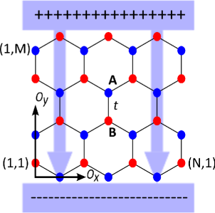
Figure 1: (Color online) A piece of honeycomb lattice with two type of edges: zig-zag (along the $\textbf{O}_{x}$ direction) and armchair (along the $\textbf{O}_{y}$ direction). The blue points belong to the sublattice A and the red points to the sublattice B, t is the hopping amplitude connecting the nearest neighbor lattice points; the static electric field (blue arrows) is applied parallel to $\textbf{O}_{y}$ axis. The number of lattice sites is $N\times M$, were $N$ is odd and $M$ is even, in our sketch $7\times 4$.

Since the honeycomb lattice arises from the overlapping of two triangular lattices A and B, the tight-binding Hamiltonian can be written in terms of creation and annihilation operators $a_{n,m}^{\dagger},a_{n,m}$ and $b_{n,m}^{\dagger},b_{n,m}$, which act on the sites of the two sublattices, correspondingly. The counting of the atoms can be done in different ways. Here, in accordance with Fig.1, the index $n$ counts the atoms along the horizontal zig-zag chains, and $m$ is the chain index ($n\in[1,N]$, $m\in[1,M]$). It turns out that for the A-sites of the blue-sublattice one has $n+m=odd$, while for the red sublattice $n+m=even$. In the presence of a perpendicular magnetic field, the hopping integral $t$ (connecting the two sublattices) acquires a Peierls phase which can be calculated by integrating the vector potential along the A-B bonds. Then, the spinless tight-binding Hamiltonian that describes the $\pi$-electrons in the graphene lattice in perpendicular magnetic field has the form:

$$H=\sum_{\begin{subarray}{c}n,m\\ n+m=odd\end{subarray}}{\epsilon^{a}a^{{\dagger}}_{n,m}a_{n,m}}+\sum_{\begin{subarray}{c}n,m\\ n+m=even\end{subarray}}{\epsilon^{b}b^{{\dagger}}_{n,m}b_{n,m}}~{}~{}~{}~{}~{}~{}~{}~{}~{}~{}~{}~{}~{}~{}~{}~{}~{}~{}~{}~{}~{}~{}$$

$$+t\sum_{n,m}\big{(}{e^{\pi i\phi(m-\frac{5}{6})}a^{{\dagger}}_{n,m}b_{n-1,m}+e^{-\pi i\phi(m-\frac{5}{6})}a^{{\dagger}}_{n,m}b_{n+1,m}}\big{)}~{}~{}~{}~{}~{}~{}~{}~{}~{}~{}~{}~{}$$

$$+t\sum_{n=odd}\sum_{m=even}{a^{{\dagger}}_{n,m}b_{n,m-1}}+t\sum_{n=even}\sum_{m=odd}{b^{{\dagger}}_{n,m}a_{n,m+1}}+H.c.,$$ (1)

where $\phi$ is the magnetic flux through the hexagonal cell measured in flux quantum units $h/e$, and the vector potential was chosen as $\vec{A}=(-By,0,0)$. The first two terms in Eq.(1) represent the atomic contributions, the next two terms describe the hopping along the zig-zag chains Note-phi , while the last ones describe the hopping between the neighboring chains.

The in-plane electric field is introduced along the $O_{y}$ direction, and it is simulated by replacing in Eq.(1) the on-site energies $\epsilon^{a,b}$ with $\epsilon^{a,b}_{n,m}=e\mathcal{E}(y_{n,m}-L_{y}/2)$, where $\mathcal{E}$ is the electric field, $y_{n,m}$ is the site coordinate, and $L_{y}$ is the length of the honeycomb lattice along the $O_{y}$ direction ($L_{y}=(3M-2)a/2$, where $a$ is the hexagon side length).

The spectral properties of the Hamiltonian depend on the boundary conditions imposed to the wave function, and the most studied case is that one of the graphene ribbon, meaning that periodic conditions are imposed along one direction only. In the next subsection, we shall discuss first the effect of the electric field on the edge states in the zig-zag ribbon, and then extend the analysis to the finite plaquette, obtained by imposing vanishing boundary conditions all around the graphene lattice. Different behaviors of the edge states can be identified in three regions of the Hofstadter spectrum. At the extremities of the spectrum, in the conventional Landau range, the modifications of the edge states are similar to those discussed already in Aldea for the case of the confined 2D electron gas. Thus, in this paper, we concentrate on the relativistic Landau range, and also on the special case of the n=0 Landau level placed at the energy $E=0$. These two ranges exhibit the specific behavior of the Dirac electrons in graphene.

II.1 Zig-zag nanoribbon: spectral properties in crossed magnetic and electric fields

In the ribbon case, the momentum $k_{x}$ is a good quantum number, and the energy spectrum will be obtained by diagonalizing a $2M\times 2M$ matrix for any momentum $k_{x}$. The resulting eigenvalues as a function of $k_{x}$ are shown in Fig.2a in the absence of the electric field and in Fig.2b for a nonvanishing electric field.

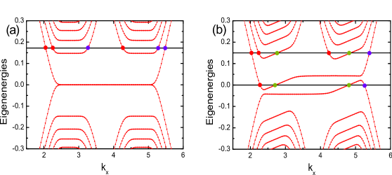
Figure 2: (Color online) The energy spectrum of a graphene zig-zag nanoribbon: (a) in the presence of perpendicular magnetic field and (b) in the presence of both magnetic and in-plane electric fields. The black lines correspond to the Fermi level and the red, blue and green dots highlight the quantum states whose corresponding conducting channels are represented in Fig.3. The theoretical simulation is performed at the following parameters: the number of sites $400\times 100$, the magnetic flux $\phi/\phi_{0}=1/500$, the electric bias $e\mathcal{E}L_{y}/t=0.1$. (These values correspond to the width $L_{y}=10l_{B}=21nm$, magnetic field $B=158T$, electric field $\mathcal{E}=1.3\times 10^{7}V/m$, and a parameter $\beta=0.09$; experimentally accessible values are suggested below by the scaling law Eq.(5).)

For the already studied case $\mathcal{E}=0$ Neto , the energy spectrum shows electron-hole symmetry with degenerate flat Landau bands, whose wave functions are located in the middle of the stripe, and dispersive states along the edges (see Fig.2a). Obviously, the non-zero velocity $v(k_{x})=\frac{1}{\hbar}dE(k_{x})/dk_{x}$ and its sign indicate the presence of currents flowing along the edges in opposite directions. For instance, choosing the Fermi level between $n=1$ and $n=2$ Landau levels, we notice 3 channels with negative velocity (marked with red dots) and other 3 channels (marked in blue) flowing oppositely on the other side of the ribbon. The picture in the real space is illustrated in Fig.3a.

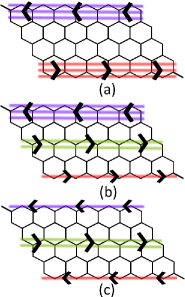
Figure 3: (Color online) Schematic representation of conducting channels in the zig-zag nanoribbon geometry corresponding to the three situations discussed in Fig.2. (a) At $\mathcal{E}=0$ there are three edge channels on each side of the ribbon, running in opposite directions. (b) At $\mathcal{E}\neq 0$ and $E_{F}=0.15$, due to the tilt of the former flat band, two channels are pushed in the middle of the stripe. (c) The special case $\mathcal{E}\neq 0$ and $E_{F}=0$ shows only four channels: unusually, the edge channels run in the same direction, while the two bulk channels run oppositely.

The additional electric field induces qualitatively new features. The former flat Landau bands get a tilt, which indicates the degeneracy lifting and a finite velocity $\frac{1}{\hbar}dE/dk_{x}$ (positive in Fig.2b for the chosen direction of the electric field). One may observe that a partial degeneracy lifting occurs also to the band $n=0$, suggesting new effects around the energy $E=0$. However, the most significant observation at $\mathcal{E}\neq 0$ is that, because of the tilt of the spectrum, the number of edge channels on the two sides of the zig-zag ribbon becomes different, and current carrying channels appear also in the middle of the stripe at the expenses of the edge channels. The number and position of the channels can be observed by counting the intersections of the Fermi level with the spectrum branches in Fig.2b. Different situations may occur depending on the position of the Fermi level in the spectrum, and two specific cases can be highlighted:
i) at $E_{f}=0.15$ we notice three edge channels on the left (stemming from n=0 and n=1 Landau levels, and marked with red dots), one edge channel on the right (stemming from n=0, marked in blue, and running in opposite direction), but also two channels (marked with green dots) coming from the inclination of the former flat band. The numerical calculation of the eigenvectors reveals that the ’green’ channels are located in the middle of the stripe as shown in Fig.3b.
ii) at $E_{f}=0$ a very interesting case occurs. Fig.2b puts into evidence two edge states (marked in red and blue) which show this time the same (negative) derivative, i.e., the same direction of the current, while the ’green’ doublet in the middle shows the opposite sign. The distribution of the channels in the real space turns out to be unusual in this case as shown in Fig.3c.

The three situations discussed for the ribbon geometry show that the location of the channels along the $O_{y}$ axis depends on the presence/absence of the electric field and on the position of the Fermi level. We are left now with the question how the channels will be distributed in the actual case of a finite rectangular plaquette.

The energy spectrum of the graphene ribbon in crossed electric and magnetic fields apparently shows in Fig.2b the symmetry $E(k^{0}_{x}+k_{x})=-E(k^{0}_{x}-k_{x})$ around a point $k^{0}_{x}$, which was also noticed in Roslyak in the frame of the continuum model. In Appendix we prove the existence and calculate the value of $k^{0}_{x}$. The proof indicates that the spectrum symmetry relies on the specific inversion symmetry of the honeycomb lattice that moves the atoms A in atoms B and vice-versa. The position of $k^{0}_{x}$ is defined modulo $\pi$ and depends on the magnetic field $B$ and the ribbon width $M$.

We continue the discussion on the graphene ribbon with considerations concerning finite size aspects and scaling properties of the energy spectrum. One knows that the two-dimensional electron gas in a perpendicular magnetic field shows the degenerate Landau spectrum and quantum transport properties if the linear dimension $L$ is much larger than the magnetic length $l_{B}=\sqrt{\hbar/eB}$ ($L>>l_{B}$). In other words, at a given $B$, the system enters the Landau quantization regime only if $L$ is sufficiently large. For the graphene ribbon, the gradual formation of the Dirac-Landau spectrum with increasing width was noticed already in Huang . We return to this problem in Fig.4a where we keep the magnetic flux fixed at $\phi/\phi_{0}=0.0005$ (corresponding to $B=39.5T$) and observe the formation of the degenerate Dirac-Landau levels when the width $L_{y}$ increases. The only level that is always present, no matter the ribbon width, is the level $n=0$. In what concerns the others $n=1,2,...$, one can see that, for instance at M=100 (when the ribbon width $L_{y}=(\frac{3M}{2}-1)a=21nm=5.2l_{B}$), the specific degenerate levels do not manifest themselves (the red curve). However, such states appear at the larger widths corresponding to M=200 and 400 ($L_{y}=42.4nm\approx 10.5l_{B}$ and $Ly=85nm\approx 21l_{B}$, respectively).

We make now a step further proving the finite size scaling behavior of the spectrum in the relativistic domain. To this aim, one calculates the energy spectrum for different widths and magnetic fields and finds a scaling function that allows the superposition of all curves into a single one as in Fig.4b. One makes first the scaling hypothesis that the relativistic Landau eigenvalues $E_{n}$ are homogeneous functions of $B$ and $L_{y}$ :

$$\lambda E_{n}(B,L_{y})=E_{n}(\lambda^{s_{1}}B,\lambda^{s_{2}}L_{y})$$ (2)

The parameter $\lambda$ is arbitrary and, with the choice $\lambda=B^{-1/s_{1}}$, one gets

$$B^{-1/s_{1}}E_{n}(B,L_{y})=E_{n}(1,B^{-s_{2}/s_{1}}L_{y}).$$ (3)

The scaling behavior shown in Fig.4b occurs for $s_{1}=2$ and $s_{2}=-2$, resulting the following scaling law:

$$E_{n}(B,L_{y})=\sqrt{B}f(BL_{y}).$$ (4)

In Fig.4c we detected also the scaling behavior of the low energy spectrum in the presence of both magnetic and electric fields. In this case, repeating the above arguments, the resulting scaling law is the following:

$$E_{n}(B,\mathcal{E},L_{y})=\sqrt{B}\tilde{f}(BL_{y},\mathcal{E}L_{y}^{3/2}).$$ (5)

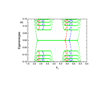
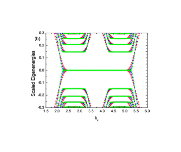
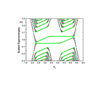
Figure 4: (Color online) (a) The gradual formation of the Dirac-Landau levels with increasing width of the graphene ribbon at $\phi/\phi_{0}=0.0005~{}(B=39.5T)$: $M=100$ (red), $M=200$ (blue), $M=400$ (green). (b) The eigenenergies scaled according to Eq.(4); the three superimposed curves correspond to $M=100,\phi/\phi_{0}=0.002~{}(B=158T)$ (red), $M=200,\phi/\phi_{0}=0.001~{}(B=79T)$ (blue), and $M=400,\phi/\phi_{0}=0.0005~{}(B=39.5T)$ (green). (c) The scaled eigenenergies according to Eq.(5) when both magnetic and electric fields are present; the sequence of curves is the same as in (b), the electric bias being $e\mathcal{E}L_{y}/t=0.1(\mathcal{E}=1.3\times 10^{7}V/m),e\mathcal{E}L_{y}/t=0.1/\sqrt{2}(\mathcal{E}=4.5\times 10^{6}V/m)$, and $e\mathcal{E}L_{y}/t=0.05(\mathcal{E}=1.6\times 10^{6}V/m)$, correspondingly.

The finite size scaling, besides being intrinsically interesting, helps to overcome technical problems met in the numerical simulations of the physical effects. Since the computer simulation of finite but large systems pretends much memory and running time, one has to consider smaller systems subjected however to external (magnetic, electric) fields higher than available experimentally. Then, the scaling law says that the same behavior is expected at smaller fields but at larger size. For instance, the data in Fig.2b are obtained at $B=158T$ and $\mathcal{E}=1.3\times 10^{7}V/m$ for a width of $L_{y}=21nm$, but the scaling law Eq.(5) shows that the same value of the scaling function would be obtained at $B=15T$ and $\mathcal{E}=4\times 10^{5}V/m$, if the width were $L_{y}=221nm$.

We note that the analysis of the finite size scaling for the graphene plaquette is technically more difficult than for the ribbon, and it will not be addressed here.

II.2 Shortcut edge states in finite plaquette geometry

The finite size plaquette can be obtained from the ribbon by imposing vanishing boundary conditions also along the $O_{x}$ direction. The resulting structure we shall consider will be like in Fig.1, the rectangular geometry showing two zig-zag and two arm-chair boundaries. Then one can assume that the channels, described above for the ribbon case, will give rise to closed circuits in the confined system. The main question is how the channels located in the middle of the stripe (shown in Figs.3b,c) will get closed in the plaquette geometry. Intuitively, they should generate channels that touch all the four edges, but also channels that get closed through the middle of the plaquette. However, the analysis performed in the previous subsection cannot be adopted now in a straightforward manner since the momentum $k_{x}$ is no more a good quantum number. So, we shall discuss the effect of the applied electric field in terms of the changes induced to the Hofstadter energy spectrum, to the bulk and edge quantum states, and to the diamagnetic response of the system.

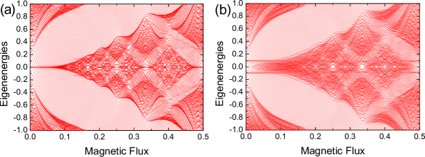
Figure 5: (a) The relativistic range of the Hofstadter spectrum for a graphene plaquette in the absence of the electric field. Edge states fill the gaps as an effect of the finite size. (b) The in-plane electric field lifts the quasi-degeneracy of the Landau bands; the most visible effect concerns the n=0 band in the middle of the spectrum. The number of lattice sites is $35\times 20$, and the electric bias is $e\mathcal{E}L_{y}/t=0.2$. (The energy is measured in units of hopping integral $t$, and the magnetic flux through the hexagonal cell in flux quanta $h/e$.)

Before discussing the energy spectrum of the confined system in crossed magnetic and electric fields, it is useful to remind some spectral peculiarities of the infinite graphene sheet in perpendicular magnetic field. In this case, the spectrum is composed of two Hofstadter butterflies containing both conventional Landau levels (which depend linearly on the magnetic field $B$) and relativistic Landau levels (which depend on the magnetic field as $B^{1/2}$). Also specific to graphene is a flat Landau level n=0 that appears in the middle of the spectrum (at $E=0$). On the other hand, in the case of the finite size graphene, the confinement induces edge states, which fill the interlevel gaps, and a slight lifting of the level degeneracy. These aspects can be noticed in Fig.5a, where the eigenvalues, obtained by the numerical diagonalization of the Hamiltonian (1) with vanishing boundary conditions, are shown as function of the magnetic flux for the relativistic (low energy) range of the spectrum. The additional effect of the in-plane electric field can be seen by inspection of Fig.5b, but, an easier examination can be done by observing the diamagnetic moments $M_{n}$ of the individual states $n$ in Fig.6. Since the sign of $M_{n}$ reveals the chirality of the state $|n>$, the diamagnetic moment is a convenient tool for probing the bulk and, respectively, the edge states, which are distinguished by their opposite chirality. The calculation of $M_{n}$ can be easily performed following the recipe described in Aldea1 .

Figure 6: The orbital magnetization $M_{n}$ of the eigenstates versus the eigenenergies $E_{n}$ for a graphene plaquette of dimension $41\times 40$, with no electric field (a), and with an in-plane electric field $e\mathcal{E}L_{y}/t=0.2$ (b), $\phi/\phi_{0}=0.03,\beta=0.03$. In the panel (b), the shortcut edge states located in the first relativistic band (see text) are marked with arrows. Alternate magnetizations are to be noticed in the zero-energy range.

The following aspects can be noticed by comparing the two panels in Fig.6:
i) the energy range occupied by the bulk states at $\mathcal{E}\neq 0$ is more extended than in the case of vanishing electric field. This is understandable since the electric field lifts the quasi-degeneracy of any Landau band, giving rise to a Stark fan with increasing field.
ii) the presence among the bulk states at $\mathcal{E}\neq 0$ of several states of reverse chirality, mentioned with arrows in Fig.6b ; their chirality indicates that the states are of edge-type, nevertheless they behave unusually. Indeed, the calculation of the charge density $|\Psi(\vec{r})|^{2}$ proves that all these states keep the localization along the edges, but exhibits also a ridge in the middle of the plaquette, which is perpendicular on the direction of the electric field, and shortcuts two opposite sides. For a given magnetic field, the position of the ridge on the plaquette depends on the energy $E_{n}$ and can be modified by changing the electric field. Such states generated by the application of the electric field, are shown in Fig.7, and will be called shortcut edge states.

In the classical picture, the normal edge states are assimilated to skipping cyclotron orbits along an equipotential line near the hard walls. In the same line of thinking, one may assume that the applied electric bias creates an internal barrier that limits the electron motion and compels the skipping orbit to close along the equipotential line along the electric barrier. This would be the classical picture of a shortcut edge state.

The diamagnetic current carried by a shortcut edge state flows along the plaquette edges, but part of it closes through the middle. When leads are attached to the plaquette, the shortcut obviously affects the electron transmittance between the different leads, with consequences for the quantum Hall effect that will be discussed in sec.III.

One cannot disregard the presence also in the left panel of Fig.6 (at $\mathcal{E}=0$) of a state of reversed chirality in the first Landau band. We checked it by calculating the charge distribution, and it turned out that the state is a usual edge state going around all the four edges of the sample. We assume that it appears accidentally among the bulk states as a finite size effect for the given plaquette, at the given magnetic field, due to some specific hidden symmetry.

At this stage one has to discuss the question of the electric field strength. It is known from the continuous approximation used in Baskaran ; Castro that, with increasing value of the parameter $\beta$, the gaps between the relativistic Landau levels diminish, and there is a critical value $\beta=1$ at which all the gaps vanish. We need to say that our results, obtained in the finite lattice model are generated for values of $\beta$ which are lower than those used in Lukose et al Baskaran and much lower than the critical $\beta$.

The closing of the gaps with increasing electric field obviously occurs also in the lattice model due to the broadening of the Dirac-Landau bands provided by the above mentioned formation of the Stark fan Note-critic . In this way, the gaps disappear together with the normal edge states located inside. However, an interesting question concerns the fate of the shortcut edge states at high values of $\beta$, beyond the gap closure. One has to remember (see Fig.6b) that the shortcut edge states appear in the bands (not in the gaps), so that one may suppose that they will survive even at high values of $\beta$, when the gaps disappear and the mixing of the adjacent bands occurs. This situation, if true, should be seen in the quantum Hall effect, which is no more carried by the normal edge states, but only by the shortcut edge states. Indeed, the calculation of the Hall resistance shows in Fig.11 that for $e\mathcal{E}L_{y}/t=0.5$ the normal plateaus disappear (except the first one corresponding to the largest first gap, which is not yet closed), but the intermediate plateaus at $R_{H}=2/3$ and $R_{H}=4/16$, supported by the shortcut edge states, still exist.

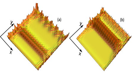
Figure 7: $|\Psi(\vec{r})|^{2}$ for two shortcut edge states from the first relativistic Landau band corresponding to the energies $E=0.5306$ (panel a) and $E=0.5786$ (panel b). The number of lattice sites is $105\times 40$, $\phi/\phi_{0}=0.03$, and $e\mathcal{E}L_{y}/t=0.2$, corresponding to $\beta=0.03$.

One may also ask the question whether the shortcut edge states are present at any small electric field or there is a threshold above which these states appear. The question is conceptually interesting since it can give a physical hint, beyond the numerical result, for the formation of the shortcut edge states. The answer is based on the discrete character of the energy spectrum of the finite plaquette and on the different response of the two types of states (band and edge) to the presence of the electric field. As we already noticed, the band states are linearly shifted on the energy scale (giving rise to the Stark fan), while the edge-type energies are robust. Consequently, there is an $\mathcal{E}$ for which a bulk state becomes resonant with the first edge state met in the gap. Up to this value of the electric field the separate character of the edge and bulk states is maintained Note-shape , however they hybridize with each other at the resonance. It turns out that the new state is a shortcut edge state, as it is proved by the numerical calculation of the charge density distribution on the plaquette. So, one concludes that for the existence of the shortcut edge states the electric field should be higher than a minimal value determined by the edge states level spacing (call it $\delta$), i.e. $e\mathcal{E}L>\delta$, where $L$ is the length of the sample in the direction of the field. Obviously, $\delta$ depends on the plaquette dimension and is different in different gaps. Since $\delta$ vanishes in the limit $L\rightarrow\infty$, the critical electric field goes to zero in the limit of large systems. In the case of the plaquette considered in Fig.6 (41$\times$40 sites corresponding to 4.9$\times$8.4 $nm^{2}$ and $\phi/\phi_{0}=0.03$), the estimated critical $\beta$ is $0.006$ in the first gap.

II.3 The special case around the energy $E=0$

One may notice in Fig.5b that the additional in-plane electric field lifts the degeneracy of the n=0 Landau level and gives rise to a broad splitting in the energy range (-0.1, 0.1). Obviously, the splitting depends on the strength of the applied electric field. The resulting states that fill this range appear in pairs of opposite chirality Note1 , fact that can be observed either looking at the derivative $dE_{n}/d\phi$ in Fig.5b or at the sign of the magnetic moments in Fig.6b. The small values of the magnetic moments in the energy range close to $E=0$ suggest that the surface encircled by the diamagnetic currents might be also small. In order to check this idea, we calculated the charge distribution $|\Psi_{n}(\vec{r})|^{2}$ on the plaquette, and a somewhat surprising result came out. Namely, all the states shortcut the plaquette, looking as in Fig.8, where two eigenstates, consecutive on the energy scale, are shown. One observes that they encircle complementary areas on the plaquette, which are controlled by the electric field intensity. This behavior, regarding both the chirality and the arrangement on the plaquette, is assigned to all states that appear in the central energy range.

The states described above represent a second kind of shortcut edge states to be found in the finite size graphene plaquette. We expect them to give new features to the transport properties near the zero-energy. We advance already the idea that the asymmetric positioning of the states on the plaquette should manifest itself in the dependence of the transport properties on the configuration of the current and voltage leads in the Hall device. The topic will be explored in the next section.

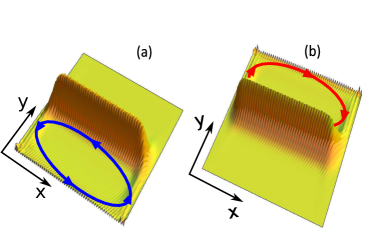
Figure 8: (Color online) $|\Psi(\vec{r})|^{2}$ for two consecutive shortcut edge states from the central Landau band (n=0) in the presence of the in-plane electric field. The states show alternate chiralities (magnetizations) which are illustrated by blue and red loops. The number of lattice sites is $105\times 40$, $\phi/\phi_{0}=0.03$, $e\mathcal{E}L_{y}/t=0.2$ and $\beta=0.03$.

III Peculiar IQHE of the graphene plaquette in the presence of the in-plane electric field

In order to reveal the specific transport proprieties of the graphene plaquette in crossed electric and magnetic fields, we simulate a quantum Hall device by attaching four leads to the graphene plaquette. In this way, we investigate the modifications produced by the in-plane electric field to the already familiar picture of the IQHE in graphene, which in the relativistic energy range shows plateaus at $R_{H}=\pm\frac{h}{e^{2}}\frac{1}{2n+1}$ (with $n=0,1,2,..$, and forgetting about the spin degeneracy). The basic idea is that the novel edge states, due to their specific properties induced by the applied bias (and discussed in the previous section), affects the electron transmittance between different leads, and, implicitly, the plateaus of the quantum Hall resistance.

It is of interest to note that the quantum Hall behavior in the two distinct domains occupied by the shortcut edge states can be guessed heuristically by exploiting the qualitative features of the edge states and the way in which they shortcut the plaquette and interconnect the leads. This approach suggests the presence of some new, specific quantum Hall plateaus, which, however, should be checked numerically.

The numerical calculation is performed in the Landauer-Büttiker formalism, the basic formulas being reminded here. In a four lead-device the charge current through the lead $\alpha$ can be written in the linear regime as:

$$I_{\alpha}=\sum_{\beta=1}^{4}~{}g_{\alpha\beta}V_{\beta},$$ (6)

where $g_{\alpha\beta}$ is the conductance matrix, $V_{\beta}$ is the potential at the contact $\beta$, and the lead indices $\alpha,\beta=1,...,4$. The current conservation and the possibility to choose arbitrarily the origin of the potential impose the conservation rules:

$$\sum_{\alpha=1}^{4}g_{\alpha\beta}=\sum_{\beta=1}^{4}g_{\alpha\beta}=0~{}.$$ (7)

For $\alpha\neq\beta$, the conductance $g_{\alpha\beta}$ can be expressed in terms of the transmission coefficients $T_{\alpha\beta}$ between the leads $\alpha$ and $\beta$ as $g_{\alpha\beta}=\frac{e^{2}}{h}T_{\alpha\beta}$ . On the other hand, the diagonal term $g_{\alpha\alpha}$ can be obtained either from the above conservation law or using the recipe $g_{\alpha\alpha}={\frac{e^{2}}{h}}(T_{\alpha\alpha}-M^{c}_{\alpha})$, where $M^{c}_{\alpha}$ is the number of channels in the lead $\alpha$. The second recipe can be immediately deduced from the Datta’s formalism in Datta .

The transmission coefficients $T_{\alpha\beta}$ can be calculated using the Green function approach. The method pretends to know the full Hamiltonian consisting of the sample Hamiltonian $H^{S}$ given in our case by Eq.(1) and supplementary terms, which describe the leads $H^{L}$ and the sample-lead coupling $H^{SL}$:

$$H=H^{S}+H^{L}+\tau H^{SL}.$$ (8)

We consider many-channel perfect leads similar to those introduced in Buettiker , the strength of the lead-sample coupling used in the numerical calculation being $\tau=2t$. The role of the leads is to inject and collect the current flowing through the graphene plaquette; in the considered tight-binding model, each lead consists of $M^{c}$ semi-infinite one-dimensional conducting chains, which are attached to consecutive sites of the plaquette. In terms of creation (annihilation) operators acting on the lead sites, the Hamiltonian $H^{L}$ reads Aldea :

$$H^{L}=\sum_{\alpha}H^{L}_{\alpha},~{}~{}~{}H^{L}_{\alpha}=t\sum_{\nu=1}^{M^{c}}\sum_{n\geq 1}c^{\dagger}_{\alpha,\nu,n}c_{\alpha,\nu,n+1}+H.c.~{},$$ (9)

where $\nu$ counts the chains, $n$ counts the sites along any semi-infinite chain, and $t$ is the hopping integral on the chain.

The transmission coefficient $T_{\alpha\beta}$, which describes the electron propagation from the lead $\beta$ to the lead $\alpha$ at the Fermi energy $E_{F}$, is given by the expression:

$$T_{\alpha\beta}(E_{F})=4\tau^{4}\sum_{\nu,\nu^{\prime}}|G_{\alpha\nu,\beta\nu^{\prime}}^{+}(E_{F})|^{2}Img_{\alpha,\nu}^{L}(E_{F})Img_{\beta,\nu^{\prime}}^{L}(E_{F}),~{}~{}\alpha\neq\beta,$$ (10)

where $G^{+}$ is the retarded Green function of the system in the presence of the coupled leads, and $g^{L}$ is the lead Green function (so that $Img_{\alpha,\nu}^{L}(E_{F})$ represents the density of states at the Fermi energy of the chain $\nu$ in the lead $\alpha$).

Next, if $V_{\alpha\beta}(\alpha\neq\beta)$ is the voltage drop measured between the contacts $\alpha$ and $\beta$ when the current $I_{\delta\gamma}$ flows between the contacts ($\delta,\gamma$), with the notation $R_{\gamma\delta,\alpha\beta}=V_{\alpha\beta}/I_{\delta\gamma}$ (introduced by van der Paw Paw for many terminal devices), the transverse (Hall) resistance of the four-terminal device sketched in Fig.9 is given by:

$$R_{H}=(R_{13,24}-R_{24,13})/2=(g_{23}g_{41}-g_{21}g_{43}-g_{32}g_{14}+g_{12}g_{34})/2D,$$ (11)

where $D$ is a $3\times 3$ subdeterminant of the conductance matrix defined in Eq.(6). We note that, since the conductance matrix satisfy the conservation rules Eq.(7), all the $3\times 3$ subdeterminants are equal (up to a sign which is irrelevant here) and different from zero.

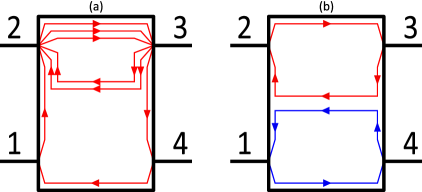
Figure 9: (Color online) The sketch of the current carrying channels when four leads are attached to the graphene plaquette. The involved shortcut edge states are those from Fig.7 in the panel (a) and those from Fig.8 in the panel (b).

The first kind of shortcut edge states was identified in Fig.6b as being dispersed among the bulk states in the relativistic Landau band broadened by the electric field. Then, we may argue that, instead of observing the expected drop of the Hall resistance between two consecutive plateaus, one may find an uncommon plateau supported by the new type of edge states located here. Such a state looks like in Fig.7, while the way it interconnects the leads is shown in Fig.9a. The distribution of the channels and their chirality (shown in Fig.9a for a given direction of the magnetic field) help in specifying $T_{\alpha\beta}$. For instance, one notices that the leads 1 and 2 are interconnected by one channel, while the leads 2 and 3 are interconnected by three channels, meaning that $T_{21}=1,T_{32}=3,T_{12}=0$, etc. Then, using also the conservation rules mentioned above, the whole 4$\times$4 conductance matrix g can be easily built up as:

$$\text{{\bf g}}=\frac{e^{2}}{h}\begin{pmatrix}-1&0&0&1\\ ~{}1&-3&2&0\\ ~{}0&~{}3&-3&0\\ ~{}0&~{}0&1&-1\end{pmatrix}.$$ (12)

The Hall resistance $R_{H}$ can be calculated now according to the Landauer-Büttiker recipe Eq.(11), the result being $R_{H}=2/3(h/e^{2})$. This value represents a new plateau placed in the relativistic domain at half the distance between the usual plateaus $R_{H}=1(h/e^{2})$ and $R_{H}=1/3(h/e^{2})$. This plateau is clearly evidenced by the numerical calculation in Fig.11. (We remind once again that the spin degeneracy is not taken into account.)

The second kind of shortcut edge states, resulting from the degeneracy lifting of the n=0 Landau level, are located in the middle of the spectrum. When calculating numerically the quantum Hall resistance, we noticed in this range some unusual features of the conductance matrix, which are listed below:

$$T_{12} = T_{21}=0,~{}~{}T_{34}=T_{43}=0,$$ (13a)

$$T_{41} = T_{32}=1,$$ (13b)

$$T_{41} = T_{14}+T_{13},~{}~{}T_{32}=T_{23}+T_{24}.$$ (13c)

These relations are quite different from the usual conditions for the realization of the conventional IQHE, which (for a single channel and a given orientation of the perpendicular magnetic field) read simply $T_{\alpha,\alpha+1}=1$ and $T_{\alpha+1,\alpha}=0$ (for any lead $\alpha$), all the other elements being zero. The Eq.(13a) and Eq.(13b) are corroborated by the properties of the edge states already observed in Fig.8, where the two states cover complementary areas of the plaquette and have opposite chirality. These features of the quantum states suggest the configuration of the channels on the plaquette sketched in Fig.9b. One may notice that the contacts 1 and 2 are not connected, meaning that both $T_{12}$ and $T_{21}$ vanish (similarly, $T_{34}=T_{43}=0$), and that the blue state connects the leads 1 and 4 in the direction providing $T_{41}=1$ (similarly, $T_{32}=1$ for the red state).

However, we are still left with the intriguing relation $T_{41}=T_{14}+T_{13}$, where $T_{13}\neq 0$, although the contacts 1 and 3 are apparently disconnected as in Fig.9b. Thus, the transmission coefficient $T_{13}$ breaks the expected symmetry $T_{14}=T_{41}$, and plays the role of a ’leakage’ between the two (red and blue) circuits. A plausible explanation for this effect might be that the states, being very close on the energy scale, can be hybridized easily by the perturbation introduced in the system by the lead-plaquette coupling $\tau$ (see Eq.(8)). In this way, the two circuits become interconnected if $\tau\sim\Delta$, where $\Delta$ is the mean interlevel distance in the corresponding energy range. Then, using this conjecture, with the notation $T_{13}=T_{24}=\delta$, and observing in Fig.9b the manner the contacts are bridged, the corresponding matrix reads:

$$\text{{\bf g}}=\frac{e^{2}}{h}\begin{pmatrix}-1&~{}0&\delta&1-\delta\\ ~{}0&-1&1-\delta&~{}\delta\\ ~{}0&~{}1&-1&~{}0\\ ~{}1&~{}0&~{}0&-1\end{pmatrix}.$$ (14)

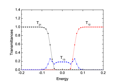
Figure 10: (Color online) Transmission coefficients vs. energy for a mesoscopic graphene in the presence of both perpendicular magnetic and in-plane electric fields. Around the zero-energy, $T_{21}=T_{12}=0$ and $T_{13}\neq 0$ evidencing the ’leakage’ between the two circuits illustrated in Fig.9b. The number of lattice sites is $51\times 100$, the magnetic flux $\phi/\phi_{0}=0.03$, electric field $e\mathcal{E}L_{y}/t=0.25$ and $\beta=0.015$.

By using again Eq.(11), we get this time the plateau $R_{H}=0$ that should become visible in the middle of the spectrum about the energy $E=0$. This value obtained by the heuristic method is also confirmed by the numerical calculation in Fig.11. The numerical values obtained for $T_{12}$, $T_{21}$ and $T_{13}$ are shown in Fig.10. The unusual behavior can be noticed indeed about $E=0$, where both $T_{12}$ and $T_{21}$ vanish, while $T_{13}$ is different from zero. Outside this energy range, $T_{13}$ vanishes (and also $T_{42}$), while $T_{12}$ and $T_{21}$ take the normal values that characterize the first relativistic gaps in the graphene Hofstadter spectrum.

The result of the numerical investigation of the Hall resistance as function of the energy in the relativistic range of the spectrum, in both the presence and absence of the applied electric bias, is shown in Fig.11. At vanishing bias, the red curve exhibits the well-known plateaus of the IQHE in graphene at $1,1/3,1/5$ (in units $h/e^{2}$). However, at $\mathcal{E}\neq 0$, the blue curve shows supplementary unconventional plateaus that appear in-between at $2/3$ and $4/15$, and also a very specific plateau at $R_{H}=0$.

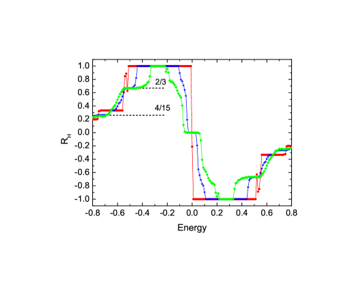
Figure 11: (Color online) Hall resistance as a function of energy with no electric field (red curve) and with electric filed $e\mathcal{E}L_{y}/t=0.25$ (blue) and 0.5 (green). We notice the appearance of the intermediate Hall plateaus in the presence of the electric field. At strong $\mathcal{E}$ (green curve) the normal plateaus at $R_{H}=1/5$ and $1/3$ disappear due to closing of the corresponding gaps in the spectrum.

(The number of lattice sites $51\times 100$ and $\phi/\phi_{0}=0.03$, $\beta=0.015$ (blue) and $\beta=0.03$ (green).)

In what concerns the longitudinal resistance, an interesting result comes from the possibility to define (and measure) it in two different ways, depending on the chosen configuration for the voltage and current terminals, namely:

$$R_{L}^{A}=(R_{23,14}+R_{14,23})/2=(g_{12}g_{43}-g_{13}g_{42}+g_{21}g_{34}-g_{24}g_{31})/2D,$$ (15)

$$R_{L}^{B}=(R_{12,34}+R_{34,12})/2=(g_{31}g_{42}-g_{32}g_{41}+g_{13}g_{24}-g_{14}g_{23})/2D.$$ (16)

Using again Eq.(14), valid in the energy range near $E=0$, one finds that the longitudinal resistance shows a dissipativeless behavior $R_{L}^{A}=0$ in the configuration $A$, but gets a finite value, which depends on the ’leakage’ parameter $\delta$, in the configuration $B$, namely $R_{L}^{B}=(1-\delta)/\delta$.

Since the numerical calculation refers to the Hall resistance of the finite graphene plaquette, it is opportune here to make some comments concerning the effect of the finite size on the structure of the Landau bands. The discussion is prompted by the fact that the Hall resistance described by the red curve in Fig.11 does not drop abruptly (as one may expect) between the plateaus $R_{H}=1$ and $R_{H}=1/3$, separated by the first Dirac-Landau band, but even shows an oscillation. The confinement represents a perturbation which, on one hand, introduces edge states in the spectrum, and, on the other hand, slightly lifts the degeneracy of the Landau states giving rise to a small band broadening. Obviously, as in any mesoscopic problem, the effect of the surface depends on the dimension of the plaquette, and , more precisely, the smaller the plaquette, the larger the broadening of the Landau bands is. However, the splitting occurs differently at different magnetic fluxes, so that, the overall aspect of the broadened band is a bunch of states exhibiting numerous anticrossing points when the magnetic field is varied. Our preliminary observations, based on the numerical calculation of the Hofstadter spectrum, indicate that the relativistic Landau bands, placed in the central part of the spectrum, are more sensitive to the confinement then the conventional Landau bands, placed at the spectrum extremities. This discussion is actually beyond the aim of the present paper and we only want to give a hint for possible unanticipated behavior of $R_{H}$ between the quantum plateaus.

As a last comment, we observe that in the presence of the electric bias, over the slight broadening due to the confinement, the broadening produced by the electric field is added (the so-called Stark ladder). Then, the transition between the successive plateaus of the Hall resistance becomes more gradual, as it can be noticed in Fig.11 (blue and green curves).

IV Summary and conclusions

In conclusion, we have proved the presence of shortcut edge states in the relativistic energy range of the mesoscopic graphene subjected to crossed magnetic and electric fields, and their influence on the transport properties denoted by new, unconventional, plateaus of the quantum Hall resistance. The novel states are defined as being only partially extended along the edges, and getting closed through the middle of the plaquette, the shortcut being controlled by the electric field.

In order to get insight on the emergence of the electrically induced shortcut states, it was helpful to study first the case of the zig-zag graphene ribbon. By applying the electric field perpendicularly to the zig-zag edges, we found that the Landau levels get tilted and, as a consequence, some of the edge channels located along the zig-zag edges are pushed by the electric field into the middle of the ribbon (as in Fig.3b). Interestingly, even the zero energy band states respond to the electric field, turning into current carrying states, some being located near the edges, and others in the middle of the ribbon (as in Fig.3c). For the graphene ribbon, we prove the scaled dependence of the low-energy Dirac-Landau spectrum on the external parameters $BL_{y}$ and $\mathcal{E}L_{y}^{3/2}$ in Eqs.(4-5).

In the case of the mesoscopic graphene plaquette, we found two kinds of shortcut edge states located differently in the relativistic range of the Hofstadter spectrum. Some of them are dispersed among the bulk states in the relativistic Landau bands, while the second type of such states arises in the middle of the spectrum due to the splitting of the n=0 Landau band induced by the electric field. In order to determine the chirality of the states, we calculated the diamagnetic moment of all quantum states in the relativistic range, with and without electric field, as shown in Fig.6.

The shortcut of the edge states created by the electric field modifies the conductance matrix in the four-lead Hall device, and gives rise to novel plateaus of the quantum Hall resistance. We presented heuristic arguments and numerical calculations for identifying the position of the new plateaus. The shortcut edge states of the first kind generate intermediate plateaus between the usual ones at $R_{H}=\pm\frac{1}{2}(\frac{1}{2n+1}+\frac{1}{2n+3})$ with n=0,1,2… (in $h/e^{2}$ units for the spinless case).

In the central part of the spectrum, the second kind of shortcut edge states come into play. They appear in pairs with different chiralities and exhibit current loops that encircle complementary areas of the plaquette, as being depicted in Fig.8. These specific properties generate the plateau $R_{H}=0$, and dissipative or non-dissipative behavior of the longitudinal resistance $R_{L}$, depending on the leads configuration.

The presented results put forward a mechanism for manipulating the transport channels in the quantum Hall regime by using an in-plane electric bias, and extend the understanding of the edge states in the relativistic energy range of the mesoscopic graphene.

V Acknowledgments

We acknowledge support from PNII-ID-PCE Research Programme (grant no 0091/2011) and Core Programme (contract no.45N/2009). One of the authors (AA) is grateful to Achim Rosch for the support in the frame of Kernprofilberech QM2 at the Institute for Theoretical Physics, University of Cologne.

*

Appendix A

As we already observed in Sec.II A, the eigenenergies of the graphene ribbon in crossed electric and magnetic fields have the symmetry $E_{k^{0}_{x}+k_{x}}=-E_{k^{0}_{x}-k_{x}}$ around a reflecting point $k^{0}_{x}$. In order to prove this property and find the value of $k^{0}_{x}$, it is appropriate to express the Hamiltonian in terms of the Fourier transforms of the creation and annihilation operators as in Neto :

$$H=\sum_{\begin{subarray}{c}k_{x},m\end{subarray}}{\epsilon^{a}_{m}a^{{\dagger}}_{k_{x},m}a_{k_{x},m}+\epsilon^{b}_{m}b^{{\dagger}}_{k_{x},m}b_{k_{x},m}+\textit{t}(e^{i\phi(m)}a^{{\dagger}}_{k_{x},m}b_{k_{x},m}}$$

$$+e^{i\phi(m)}e^{-ik_{x}}b^{{\dagger}}_{k_{x},m}a_{k_{x},m}+b^{{\dagger}}_{k_{x},m+1}a_{k_{x},m}+H.c.),$$ (17)

where $m$ labels the unit cells along the Oy-direction (m=1,..,M). The magnetic field manifests itself in the Peierls phases $\phi(m)$, while the electric field enters the atomic energies $\epsilon^{a,b}_{m}$. Applying the electric bias symmetrically on the width of the ribbon, and using the known inversion symmetry with respect to the middle of the hexagonal lattice (which moves the atoms A in the atoms B and vice-versa), the atomic energies satisfy the relation:

$$\epsilon^{a}_{M+1-m}=-\epsilon^{b}_{m}.$$ (18)

Let us measure the momentum $k_{x}$ from a not yet specified origin $k^{0}_{x}$, and let the function:

$$\Psi_{k_{x}^{0}-k_{x}}=\sum_{m}\alpha(k^{0}_{x}-k_{x},m)a^{\dagger}_{k^{0}_{x}-k_{x},m}|0>+\beta(k^{0}_{x}-k_{x},m)b^{{\dagger}}_{k^{0}_{x}-k_{x},m}|0>$$ (19)

be an eigenfunction of the Hamiltonian, such that:

$$H\Psi_{k^{0}_{x}-k_{x}}=E_{k^{0}_{x}-k_{x}}\Psi_{k^{0}_{x}-k_{x}}.$$ (20)

The objective is now to find an unitary operator $P$ with two properties:
i) to anticommute with $H$, i.e.,  $PHP^{-1}=-H$,
ii) to move the function $\Psi_{k^{0}_{x}-k_{x}}$ into another function depending on $k^{0}_{x}+k_{x}$, i.e.,  $P\Psi_{k_{x}^{0}-k_{x}}=\tilde{\Psi}_{k_{x}^{0}+k_{x}}$.
Then, applying the operator $P$ to the left of Eq.(A.4), and using the first property, one gets obviously:

$$H\tilde{\Psi}_{k_{x}^{0}+k_{x}}=-E_{k^{0}_{x}-k_{x}}\tilde{\Psi}_{k_{x}^{0}+k_{x}},$$ (21)

meaning that $E_{k^{0}_{x}+k_{x}}=-E_{k^{0}_{x}-k_{x}}$.

Taking advantage of the mentioned inversion symmetry of the lattice, we may guess the operator $P$ as:

$$P=\sum_{\begin{subarray}{c}k_{x},m\end{subarray}}{e^{-i\lambda^{b}(k^{0}_{x}-k_{x},m)}b^{{\dagger}}_{k^{0}_{x}-k_{x},M+1-m}a_{k^{0}_{x}+k_{x},m}}$$

$$-\sum_{\begin{subarray}{c}k_{x},m\end{subarray}}{e^{-i\lambda^{a}(k^{0}_{x}-k_{x},m)}a^{{\dagger}}_{k^{0}_{x}-k_{x},M+1-m}b_{k^{0}_{x}+k_{x},m}}.$$ (22)

The phases $\lambda^{a,b}$ and the reflecting point $k^{0}_{x}$ result from the condition $[H,P]_{+}=0$. After lengthy but straightforward calculations one obtains the value $k^{0}_{x}=\phi(M)+\phi(1)$ (modulo $\pi$), which depends on the magnetic field $B$ and the width of the ribbon $M$.

It is interesting to notice that performing the inverse Fourier transformation of the operators in Eq.(A.6), namely $a^{{\dagger}}_{k_{x},n}=\frac{1}{\sqrt{N}}\sum_{n}e^{ik_{x}n}a^{{\dagger}}_{n,m}$ (and similarly for the $b$ operators), one obtains an operator $\mathcal{P}$ which acts in the direct space as an inversion operator with respect to middle of the sample:

$$\mathcal{P}a^{{\dagger}}_{n,m}|0> = e^{-i(2n+m)k^{0}_{x}}b^{{\dagger}}_{N+1-n,M+1-m}|0>$$

$$\mathcal{P}b^{{\dagger}}_{n,m}|0> = -e^{-i(2n+m-1)k^{0}_{x}}a^{{\dagger}}_{N+1-n,M+1-m}|0>,$$ (23)

where $n$ and $m$ are the cell indexes $n\in[1,N]$ and $m\in[1,M]$. Thus, one may say that the symmetry of the spectrum about $k^{0}_{x}$ is the consequence of the inversion symmetry in the direct space of the hexagonal lattice.

Finally, we remark that the symmetry $E_{k^{0}_{x}+k_{x}}=E_{k^{0}_{x}-k_{x}}$ shown by Fig.2a in the absence of the electric field (but at non-zero magnetic field) can be proved in a similar way, looking for an operator $P$ that this time commutes with the Hamiltonian. In this case, $P$ looks like in Eq.(A.6) but with the plus sign between the two terms. We also note that at $\mathcal{E}=0$ all the atomic energies are equal $\epsilon^{a,b}_{m}=0$, fact that helps to attain the commutation relation $[H,P]_{-}=0$ (for which the relation $\epsilon^{a}_{M+1-m}=\epsilon^{b}_{m}$ is needed). The resulting reflecting point $k^{0}_{x}$ is the same as in the previous case.

References

- (1) C. L. Kane and E. J. Mele, Phys. Rev. Lett. 95, 226801 (2005).
- (2) K. S. Novoselov, A. K. Geim, S. V. Morozov, D. Jiang, M. I. Katsnelson, I. V. Grigorieva, S. V. Dubonos, and A. A. Firsov, Nature 438, 197 (2005).
- (3) Z. Jiang, Y. Zhang, Y.-W. Tan, H. L. Stormer, and P. Kim, Solid. State. Comm. 143, 14 (2007).
- (4) M.O. Goerbig, Rev. Mod. Phys. 83, 1193 (2011).
- (5) N. M. R. Peres, A. H. Castro Neto, and F. Guinea, Phys. Rev. B 73, 195411 (2006).
- (6) K. Nakada, M. Fujita, G. Dresselhaus, and M. S. Dresselhaus, Phys. Rev. B 54, 17954 (1996).
- (7) L.Brey and H. A. Fertig, Phys. Rev. B 73, 235411 (2006).
- (8) I. Romanovsky, C. Yannouleas, and U. Landman, Phys. Rev. B 83, 045421 (2011).
- (9) L. Malysheva and A. Onipko, Phys. Rev. Lett. 100, 186806 (2008).
- (10) T. Kramer, C. Kreisbeck, V. Krueckl, E. J. Heller, R. E. Parrott, and C.-T. Liang, Phys. Rev. B 81, 081410(R) (2010).
- (11) B. Ostahie, M. Niţă, and A. Aldea, Phys. Rev. B 89, 165412 (2014).
- (12) A. Aldea, P. Gartner, A. Manolescu, and M. Niţă, Phys. Rev. B 55, R13389 (1997).
- (13) D. A. Abanin, K. S. Novoselov, U. Zeitler, P. A. Lee, A. K. Geim, and L. S. Levitov, Phys. Rev. Lett. 98, 196806 (2007).
- (14) E. Shimshoni, H. A. Fertig, and G. V. Pai, Phys. Rev. Lett. 102, 206408 (2009).
- (15) J. Wang, B. Lian, H. Zhang, and S-C. Zhang, Phys. Rev. Lett. 111, 086803 (2013).
- (16) J.Wang, B.Lian, and S-C. Zhang, Phys. Rev. B 89, 085106 (2014).
- (17) F. Ortmann and S. Roche, Phys. Rev. Lett. 110, 086602 (2013).
- (18) M. Kharitonov, Phys. Rev. B 85, 155439 (2012).
- (19) V. Lukose, R. Shankar, and G. Baskaran, Phys. Rev. Lett. 98, 116802 (2007).
- (20) N. M. R. Peres and E. V. Castro, J. Phys.: Condens. Matter 19, 406231, (2007).
- (21) H. K. Kelardeh, V. Apalkov, and M. I. Stockman, Phys. Rev. B 90, 085313 (2014).
- (22) The Peierls phase is obtained by integrating the vector potential along the A-B bond, and the result depends on the chosen position of the coordinates origin. The phase in Eq.(1) corresponds to the origin specified in Fig.1. Of course, the energy spectrum is independent of the choice of the coordinate origin.
- (23) A. H. Castro Neto, F. Guinea, N. M. R. Peres, K. S. Novoselov and A. K. Geim, Rev. Mod. Phys. 81, 109 (2009).
- (24) O. Roslyak, G. Gumbs and D. Huang, Phil. Trans. R. Soc. A 368, 5431 (2010).
- (25) Y. C. Huang, M. F. Lin and C. P. Chang, J. Appl. Phys. 103, 073709 (2008).
- (26) A.Aldea, V. Moldoveanu, M. Niţă, A. Manolescu, V. Gudmundsson, and B. Tanatar, Phys. Rev. B. 67, 035324 (2003).
- (27) It is difficult to estimate the critical in this case because of the additional level broadening due to confinement.
- (28) During the increase of , the bulk state distorts itself: it is squeezed in the direction parallel to the field and stretches perpendicularly. At the resonance, the state meets the edge and the ’shortcut edge state’ is created.
- (29) This is a confirmation of the dual electron/hole origin of the states in the Landau level.
- (30) S. Datta, Electronic Transport in Mesoscopic Systems (Cambridge University Press, 1995), chapter 3.
- (31) M. Büttiker, Y. Imry, R. Landauer, and S. Pinhas, Phys. Rev. B 31, 6207 (1985).
- (32) L. J. van der Pauw, Philips. Res. Repts 13, 1 (1958).