Spectral Invariants in Lagrangian Floer homology of open subset
Abstract.
We define and investigate spectral invariants for Floer homology of an open subset in , defined by Kasturirangan and Oh as a direct limit of Floer homologies of approximations. We define a module structure product on and prove the triangle inequality for invariants with respect to this product. We also prove the continuity of these invariants and compare them with spectral invariants for periodic orbits case in .
Keywords: Lagrangian submanifolds, Floer homology, spectral invariants
MSC[2010] Primary 53D12, Secondary 53D40
1. Introduction
1.1. Spectral invariants in cotangent bundles
Spectral invariants in Symplectic Topology in terms of generating functions for Lagrangian submanifolds of cotangent bundles were introduced by Viterbo in [37]. If is a smooth vector bundle over a compact smooth manifold , a generic smooth function and
(here denotes the derivative along the fibre), then
is a smooth Lagrangian immersion. It is known that all Hamiltonian deformations of zero section can be generated by some function in this way [19, 6, 7]. Viterbo defined spectral invariants as a certain minimax values of . He used them to prove several important results about Hamiltonian diffeomorphisms.
In [27, 28] Oh defined spectral invariants for the case of cotangent bundle using the “homologically visible” critical values of the action functional
where is the Liouville form on . More precisely, let be a zero section of and , where is a time–one–map generated by a Hamiltonian . Let denotes the filtrated homology defined via filtrated Floer complex:
These homology groups are well defined since the boundary map preserves the filtration:
due to well defined action functional that decreases along its “negative gradient flows”. For a singular homology class define
where
is the homomorphism induced by inclusion and
is an isomorphism between singular and Floer homology groups. The construction for spectral invariants in case of conormal bundle boundary condition is done in [27], and in [28] for cohomology classes. It turned out that Oh’s invariants and the Viterbo’s ones, are in fact the same, see [21, 22].
Oh proved in [27] that these invariants are independent both on the choice of almost complex structure (which is used in the definition of Floer homology) and, after a certain normalization, on the choice of as far as . Using these invariants , Oh derived the non–degeneracy of Hofer’s metric for Lagrangian submanifolds, the result earlier proved by Chekanov [8] using different methods. Another application to Hofer geometry is given in [23, 24] in the characterization of geodesics in Hofer’s metric for Lagrangian submanifolds of the cotangent bundle via quasi–autonomous Hamiltonians.
Spectral invariants in cotangent bundles were also studied by Monzner, Vichery and Zapolsky in [26].
1.2. Beyond cotangent bundles
Spectral invariants in general symplectic manifolds have been studied by several authors, and are still the subject of active research. Without attempting to give a complete references, we mention just a few. The construction of spectral invariants for contractible periodic orbits when is a symplectic manifold with and was carried out by Schwarz (see [36]). In [20], Leclercq constructed spectral invariants for Lagrangian Floer theory in case when is a closed submanifold of a compact (or convex in infinity) symplectic manifold and , where is Maslov index. Symplectic invariants were further investigated by Eliashberg and Polterovich [11], Polterovich and Rosen [32], Oh [30], Humilière, Leclercq and Seyfaddini [13], by Monzner, Vichery and Zapolsky [26], Lanzat [18] and also in [9], [21, 22, 23, 24].
1.3. Overview of the paper
The above mentioned (and other) previous results concerning spectral invariants dealt either with Hamiltonian on symplectic manifold or with Lagrangian submanifold, thus they have a global character. Our result generalizes earlier constructions to the case of arbitrary open subsets of a base of cotangent bundle. We define spectral invariants in this case, and study how they intertwine with certain direct limits used in a construction.
Lagrangian Floer homology for open subsets in cotangent bundles was introduced by Kasturirangan and Oh in [15] as a part of a project of “quantization of Eilenberg–Steenrod axioms” (see [14]). The construction goes as follows. Let be an open subset of a compact smooth manifold , with a smooth compact boundary . The conormal bundle, , defined as
is a Lagrangian submanifold of the cotangent bundle . Define
and
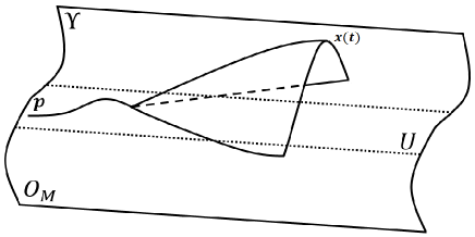
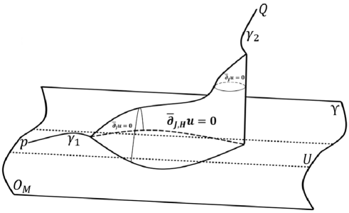
The set , called the (negative) conormal to , is a singular Lagrangian submanifold, but it allows a smooth approximation by exact Lagrangian submanifolds. Let us outline a construction of these approximations, denoted by , following [15]. For , , and are sketched in Figure 1.

In general case, denote by a tubular neighbourhood of . Since it holds:
we have:
Now if is a singular curve in :
then
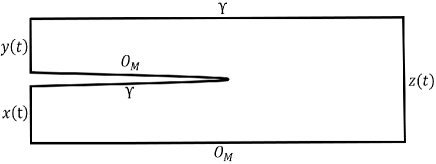
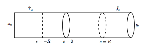
As in [15], denote by a smooth approximation of as shown in Figure 2 and define:
To show that is exact, define a function as follows:
-
•
on : is equal to zero;
-
•
on the intermediate region of : is the area of the shaded region in Figure 2 (bounded by , -axis and the line );
-
•
on : equals to the area bounded by the -axix, -axes and the curve .
It is easy to check that , where is a canonical Liouville form on and that as in Lipschitz topology (see also [15] for more details).

Floer homology for the open set is defined to be a direct limit of Floer homologies of approximations. In order to have the latter well defined, one needs to choose a compactly supported Hamiltonian such that
and
| (1) |
Both of the above conditions can be obtained by generic choice of . Floer homology for the pair is now defined in a standard way, the set of the generators consists of the Hamiltonian paths
| (2) |
which are critical points of the effective action functional:
| (3) |
The boundary map is defined by a number of perturbed holomorphic discs with boundary on and :
| (4) |
Here is an almost complex structure compatible to the standard symplectic form , which coincides with the canonical almost complex structure on at infinity. By the canonical almost complex structure we assume the one induced by the Levi-Civita connection for a fixed metric .
Denote by the corresponding Floer homology (grading is given by Maslov index, see Subsection 2.1).
Floer homology of the open subset is defined as a direct limit of above Floer homologies for the approximations :
| (5) |
after defining an appropriate partial ordering to the set of pairs (see Section 2 below or [15] for more details). The symbol in indicates that we are dealing with the negative conormal. Defined in this way, Floer homology is isomorphic to singular homology . More precisely, for a special choice of Morse function , such that points outward , Floer homology is isomorphic to Morse homology , which, in turn, is isomorphic to .
Unlike in the paper [15], we have also to deal with the positive conormal to , defined as:
where
We define Floer homology in this case in the same way, as a direct limit of Floer homologies for approximations, but now, this limit will be isomorphic to the relative homology . Again, this isomorphism is realized via Morse homology , with the different choice of (with the gradient field now pointing inward at ). The two Floer homologies and are related via Poincaré duality:
(see Subsection 2.1 for the details).
The main aim of the paper is the construction of PSS isomorphism and the investigation of spectral invariants for the Floer homology of the open subset.
The first step in this direction is the construction of Piunikhin-Salamon-Schwarz isomorphism between (respectively ) and singular homology of (respectively relative homology ) modelled by Morse homology. We will first construct PSS homomorphism for approximations. Morse homology for open subset is well defined for a fixed Morse function and a generic choice of Riemannian metric , without any direct limit construction. However, in order to obtain all transversality conditions for moduli spaces of mixed type that figure in PSS homomorphisms for approximations, we have to choose (a priori) different Riemmanian metric for different . Therefore we will also consider Morse homology as a direct limit:
(see Section 2.)
More precisely, in Section 2 we prove the following theorem.
Theorem 1.
Let be two Morse functions from a special class of Morse functions (see Definition 4 in Section 2). There exist PSS-type isomorphisms
which are natural with respect to canonical isomorphisms in Morse and Floer theory. More precisely, if
denote the canonical isomorphisms in Floer and Morse theory respectively, and and the corresponding PSS homomorphisms, then the diagram
commutes, and the same holds for the isomorphism .
We construct PSS homomorphisms and prove Theorem 1 in Section 2. First we construct the corresponding homomorphisms for approximations and prove that they commute with the homomorphisms that define the direct limit (5).
Next, we construct three pair-of-pants type products in Morse and Floer theory for open sets. Products in Morse and Floer theory were studied by various authors: Abbondandolo and Schwarz [2], Auroux [5], Oh [28] and also in [17].
Here we establish the following products for open subset.
Theorem 2.
There exist a pair-of-pants type products:
that turns Floer homology for an open set into a module. The above products satisfy:
where is a PSS isomorphism from Theorem 1.
Theorem 2 is proven in Section 3. Since Floer homology for the open set is defined as a direct limit, the key step is to prove that the products defined on homology for approximation commute with the homomorpshisms that define the direct limit.
Finally, using the above PSS isomorphism, we construct the spectral invariants for Lagrangian Floer homology of the open subset .
We prove the following properties of these spectral invariants: their continuity with respects to and their subadditivity with respect to the products from Theorem 2. We also compare the above spectral invariants with the invariants for periodic orbits case, using the homomorphisms defined via “chimneys” introduced by Abbondadolo and Schwarz [1], and Albers [3]. Further, we prove the inequality of spectral invariants between two open sets and a specific singular homology class (see Subsection 4.1). This slightly generalizes a result by Oh [29] for a spectral invariant
More precisely, in Section 4 we prove the following theorem.
Theorem 3.
For given singular or Morse homology class , the spectral invariant defined via PSS isomorphism from Theorem 1 has the following properties:
-
(A)
triangle inequality. For it holds:
-
(B)
continuity. relative spectral invariant is continuous with respect to the Hofer norm of
-
(C)
comparison with periodic orbit invariants. Let stands for a spectral invariants for periodic orbit case in , is a homomorphism in homology induced by the inclusion map, and is the map obtained by inclusion map and Poincaré duality map:
Suppose that the Hamiltonian satisfies the conditions from Frauenfelder-Schlenk’s paper [12] (see also Subsection 4.4 on page 4.4). Then it holds:
-
(D)
invariants for subsets. Let be two open subset of and let
(the homomorphism induced by inclusion ) be surjective. For it holds:
-
(E)
If and are two compactly supported Hamiltonians generating the same time-one-map, i.e. , then the corresponding invariants are the same:
so we can define for a Hamiltonian diffeomorphism .
2. PSS isomorphism
PSS type isomorphism was originally constructed by Piunikhin, Salamon and Schwarz [31] for periodic orbit case, and later adapted in [16, 3] for Lagrangian case.
One of the nice consequences of the existence of PSS isomorphism is, for example. the commutativity of the diagram:
In order to establish the similar naturality for several homomorphisms and operators in our case, we have to carefully investigate the subtleties related to the passing to direct limit. We start with the approximations and then pass to the limit.
2.1. Isomorphism for approximations
We first establish the PSS homomorphism for approximations for negative conormal case. It follows from (1) that all solutions of Hamiltonian equation with satisfy , so by choosing to coincide with outside the small neighbourhood of , we may assume that all solutions of (2) satisfy
| (6) |
The grading for is defined to be
where is a canonically assigned Maslov index, defined for any smooth closed submanifold (see Definition 5.9 in [27]). The dimension of the space of perturbed holomorphic discs that satisfy (4) and the infinity boundary conditions:
is
for all (see [15]).
Definition 4.
For a given Riemannian metric on , let be the set of all Morse functions on such that
-
•
, where is some neighbourhood of ;
-
•
the gradient vector field of is everywhere transversal to and points outward along .
Define also
Now let , and . Define the space of mixed objects (see Figure 3):
where is a smooth function such that
| (7) |
Let denotes the Morse index of a critical point .
Proposition 5.
For generic choices the set is a smooth manifold of dimension .
Proof: Let and be a half-strip . Denote by be a completion of a tangent space of:
| (8) |
which is
| (9) |
in Sobolev norm:
By in (8) and (9) we mean smooth on interior of and continuous on . Banach space gives rise to Banach manifolds of mappings by
We choose a metric as in [15] in such a way that it becomes a product metric on a tubular neighbourhood of :
Since symplectically splits into
the choice of gives rise to the splitting of vertical and horizontal spaces:
Now let and the solution of
| (10) |
Let . We fix a trivialization
and extend it to a trivialization
that preserves the splitting
The choice of provides the splitting
The operator defined as
is a section of a suitable vector bundle over . Denote its covariant linearization at by . The operator is a Cauchy-Riemann type operator acting on
where
Now we proceed as in Appendix in [28] to conclude that, for generic choice of , the set of satisfying (10) is a smooth manifold of dimension .
Denote by the unstable manifold of . For a generic choice of parameters the evaluation map
is transversal to the diagonal, so
is a smooth manifold of codimension in . Since (see [25]) and , the dimension of is
∎
Define to be the set of all solutions of the differential equation
modulo action and, similarly, denote by
| (11) |
Proposition 6.
For generic choices of parameters the following is true.
-
(1)
If , then the zero-dimensional manifold is compact, and hence, finite sets.
-
(2)
For , the topological boundary of the one-dimensional manifold is
where the first union is taken over all , with , and the second over all , such that .
Proof. The proof follows from standard arguments, using the Arzela-Ascoli and Gromov compactness theorems. Bubbling cannot occur due to exactness of and exact Lagrangian boundary conditions. Our choice of a Morse function guarantees that there are no additional boundary components coming from the sequences , since it is isolated from the boundary .∎
The part (1) in the previous proposition enables us to define the homomorphism between Morse and Floer homology. Denote by
(i.e. vector spaces over the sets of generators of corresponding indices). Let and denote the corresponding Morse and Floer homology groups.
Denote:
and define
Before we define the homomorphisms , we need to describe Floer homology construction in positive conormal case.
As in [14], we consider the anti-symplectic involution
| (12) |
Note that maps the negative conormal to the positive conormal . If is an exact Lagrangian approximation of , then is an exact Lagrangian approximation of . Next, if we define
we have
We also have an identification of the space of perturbed holomorphic discs defining the boundary operation:
so induces a Poincaré dual isomorphism:
Remark 7.
Anti-symplectic involution also induces the Poincaré dual in Morse case, since
As in Proposition 5 we conclude that the set is a smooth manifold of dimension , compact in the dimension zero and with the similar description of a boundary in the dimension one:
For , denote by and define:
The proof of the following theorem follows from the standard cobordism arguments, the part (2) of the Proposition 6 and the description of from above.
Proposition 8.
The homomorphism and induce homomorphisms
| (14) |
and
| (15) |
on the homology level, for .
If , then , so for such we have well defined both
By Poincaré duality in Morse homology we mean the isomorphism:
| (16) |
Theorem 9.
The diagram
commutes and therefore, the homomorphisms and are isomorphisms.
Proof: We need to prove
For it holds:
Obviously , where
The number is a cardinality of zero-dimensional manifold:
| (17) |
The rest of the proof relies on standard cobordism arguments. The manifold (17) is one component of the boundary of an auxiliary one-dimensional manifold:
where is a symmetric cut-off function:
The second boundary component is
and the remaining components are such that induce zero mappings in homology level. This means that the mapping is equal to
where is a cardinality of . Now, by standard cobordism arguments one shows that the latter mapping does not depend on on the homology level. Therefore we can choose and obtain holomorphic map with the boundary on , so it must be constant due to the exactness of both Lagrangian submanifolds and the fact that . Hence is chain homotopic to the map obtained by counting the pairs with properties:
The trajectory is a negative gradient trajectory of connecting two critical points of the same Morse index. Number of such pairs is equal 1 in case and 0 otherwise. Therefore, is chain homotopic to the homomorphism . ∎
For two Morse functions , Morse homologies and are canonically isomorphic (see [35]). Similarly, for two Hamiltonians and , the corresponding Floer homologies and are isomorphic (see [15]). Denote these canonical isomorphisms by
Note that we use the same notation, and , for canonical isomorphisms for two Morse homologies (relative and absolute one, i.e. for Morse functions from both and ) and two Floer homologies (negative and positive conormal case).
Theorem 10.
The diagrams
| (18) |
and
commute.
Proof: The homomorphism is the same as the map defined on generators as
where is the cardinal number (modulo ) of zero-dimensional component of the smooth manifold
Indeed, to see this, consider the boundary of one-dimensional auxiliary manifold
Similarly, is the same as the map
where is the number of zero-dimensional component of the smooth manifold
where is Hamiltonian function satisfying
So we need to proof that the maps and are the same in homology level.
Fix . Let be a homotopy connecting and
2.2. Isomorphism for Floer homology of open set
In order to define Floer homology for the open set as a direct limit of Floer homologies for the approximations, Kasturirangan and Oh defined a partial ordering on the set of approximations as:
The function is defined by on , where is a smooth function such that (recall that is exact) and is a canonical projection. Since is fixed, one has to vary the almost complex structure to obtain a generic condition for Fredholm theory. Denote by an almost complex structure corresponding to and denote by
a canonical homomorphism that satisfies:
for given triple sufficiently close to (see [15]). As we have mentioned in Introduction, Floer homology for an open subset , modelled by negative conormal, is defined as
Since we want to establish an isomorphism between Floer homology and Morse homology for a fixed Morse function, we will vary Riemannian metric, so the term “generic choices” in the Proposition 1 refers to an almost complex structure and Riemannian metric .
Fix a Hamiltonian function and a Morse function . For a Lagrangian approximation , choose an almost complex structure and a Riemannian metric such that all the transversality conditions are fulfilled, i.e. the sets , , and are manifolds for all and all Hamiltonian paths with boundaries on and . For two Riemannian metric and there is a canonical isomorphism
satisfying
This functoriality allows to consider the set as a directed system and to define Morse homology as a direct limit:
where
for some . The set obviously has a vector space structure and is isomorphic to all .
Consider a diagram:
| (19) |
where we use the abbreviations
and so on.
Proposition 11.
The diagram (19) commutes.
Proof: The homomorphism at the chain level (we denoted by the induced homomorphism in homology) is defined via the cardinal number of the set
| (20) |
and the homomorphism via the number of elements in
| (21) |
Here:
-
•
is a monotone homotopy for such that
(22) (by monotone homotopy we mean )
-
•
is a corresponding family of generic almost complex structures;
-
•
is a homotopy of Riemannian metrics such that
The rest proof of Proposition 11 relies on cobordism arguments, similarly to the proof of Theorem 10, so we omit the details.∎
We have the similar partial ordering for the set of approximations of positive conormal. Actually, we define such a partial ordering via anti-symplectic involution:
where is defined in (12). We define Floer homology for an open subset , modelled by positive conormal, as
Let denote the canonical isomorphism for the positive conormal:
defined in the same way as , by the number of solutions of (21) (see also [15]).
Theorem 12.
There exist direct limit homomorphisms
| (23) |
and
∎
Proof. The diagram
| (24) |
commutes. This can be proved in the same way as Proposition 11. Now the proof follows directly from Proposition 11 and the commutative diagram (24). ∎
The Poincaré duality isomorphism defined in (16) obviously commutes with the maps , being defined as . Hence it induces an isomorphism on a direct limit Morse homology . Denote it again by
In order to emphasize the particular Riemannian metric we will use the notation:
Regarding the Floer case, it is easy to see that
so defines the map
Again, denote:
Theorem 13.
The diagram
commutes and therefore, the induced maps and are isomorphisms.
∎
From the canonical isomorphisms
and the commutativity of the diagrams
(and similarly for the positive conormal) we obtain isomorphisms:
Similarly, we have
Theorem 14.
The diagram
commutes and the same holds for the other PSS isomorphisms, and .
Proof: Recall that the diagram (18) commutes for all approximations close enough to and for generic choices. So we have
for every . ∎
This proves Theorem 1.
3. Product on homology and module structure
In this section we construct a product on Floer homology for an open subset, a product on Morse homology, and a product which turns Floer homology to a module over a Morse homology ring. We also prove the compatibility of PSS isomorphisms with the above product and thus we prove Theorem 2.
3.1. Product on homology
First we construct a product on Floer homology for an open subset
In order to do that, we need to define a product on homology for approximation
| (25) |
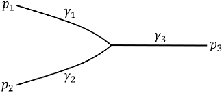
and to check its compatibility with direct limit homomorphisms. A product (25) is defined by a number of pair–of–pants objects. More precisely, let be a Riemannian surface (with a boundary)
with the identification for (see Figure 4).
Denote by , , the three ends
and by , . Let denote the smooth cut–off function such that
For , and we define a moduli space
(see Figure 4).
For generic choices, is a smooth –dimensional manifold. For two generators and of Floer homology, a map is defined as
where, denotes the (modulo 2) number of elements of a zero-dimensional component of . We extend the product to
by bilinearity. By standard cobordism arguments, one can show that commutes with boundary maps and induces a product in homology (25).
The following lemma provides the compatibility of the product with the direct limit homomorphisms. Recall that we denote by the homomorphism
defined by (21). Here , etc. To emphasize the Hamiltonian, we will write .
Lemma 15.
For , it holds
| (26) |
Proof. The homomorphism is an isomorphism for , large enough. The inverse homomorphism is actually (defined as in (21), despite the reversed order of and ). This can be proved using exactly the same cobordism arguments similar to ones in the proof of the independence of Floer homology with respect to the parameters (Hamiltonian, almost complex structure). Therefore, (26) is equivalent to
| (27) |
In order to prove (27), consider the following auxiliary one-dimensional manifold. Let be as in (22) and , , be the solutions of
For , define to be the set of all solutions of the equation
where is depicted in the Figure 5, as well as corresponding boundary conditions. The almost complex structure is chosen to satisfy all the regularity conditions.
Define to be the set of all pairs , where and .

Now the boundary of one dimensional component of is the union of the following five strata (recall denotes the space of unparametrized trajectories defining the boundary operator in Floer homology, see (11) and is defined in (21)):
The operations induced by the number of elements of boundary strata , and are zero in the homology, and the operations defined by the cardinality of and of are equal to and on the homology level. ∎
Now we are able to define the product on the direct limit homology group.
Proposition 16.
The product defines a product on Floer homology for open subset:
Proof. Let and be the classes of elements and in a direct limit. In general, and are not the same, but, since and represent the same element in we can take and as representatives of and respectively. Therefore we can assume that and belong to some and , for the same . We now define a product in homology as
We need to check that a product does not depend on representatives of a class. Let and represent the same element in and similarly and in . This means that there exist homomorphisms
such that
Let . We have
which means that and represent the same element in .∎
3.2. Morse homology ring
Let us recall the construction of the homology product on . Let be three Morse functions such that for every critical point of . For , , we define the moduli space to be the set of all trees such that
For generic choice of these spaces are manifolds of dimension
If denotes the mod 2 number of a zero–dimensional component, then the product is defined at the chain level:
as:
on generators. The choice of Morse functions (see the Definition 4 of ) provides that the loss of compactness of is possible only as the breaking of trajectories inside . Therefore commutes with the Morse boundary operator and it is well defined at the homology level:
It is also well defined as a product on a direct limit homologies:
since it holds:
| (28) |
The latter equality can be proved in the similar way as Lemma 15.
The following proposition establishes the ring structure PSS isomorphism.
Proposition 17.
Proof: It follows from the definition of and Proposition 16 that it is enough to show that
| (29) |
for a fixed approximation and fixed Riemannian metric defining the product . The equality (29) is equivalent to
and, by Theorem 9 the latter equality is equivalent to
| (30) |
The equality (30) follows from cobordism arguments similar to ones used in the proof of Theorem 9, Proposition 11 and Lemma 15. The auxiliary one-dimensional manifold we use here is explained by Figure 7.

∎
3.3. Module structure
Let . For every approximation , we can define an external product
by a number of a suitable mixed-type objects. More precisely, let denotes a smooth family of Hamiltonians such that
For , let be a moduli space of pairs such that
The dimension of equals to
and the zero–dimensional component is compact. Now define a product on the set of the generators of chain complexes as:
where denotes the cardinality of the zero–dimensional component of . Using standard cobordism arguments, as above, one can show that induces a product in homology. Similarly to [20] one shows that
| (31) |
for all and .
In order to have the products and well defined on a direct limit of Morse and Floer homology groups, we need to check their compatibilities with homomorphisms and .
Lemma 18.
The proof is similar to the proof of Lemma 15.
This proves Theorem 2.
4. Spectral invariants
In this section we define spectral invariants for open subset and prove their properties listed in Theorem 3. We define spectral invariants via PSS isomorphism constructed in Section 2, but they can be defined alternatively, as a limit of spectral invariants for the approximations (see Proposition 20 below). This alternative definition of spectral invariants will be the key ingredient in the proof of some properties from Theorem 3.
4.1. Invariants for the open subset
In the rest of the paper we will only consider Floer homology for approximations and open set in the negative conormal case, as well as the corresponding PSS isomorphisms
for . Therefore, we will omit the sign in , in order to simplify notations.
If we consider restricted to
we have
Recall that the filtered Floer homology groups for approximations are defined as homology groups of the filtered chain complex
Since the action functional decreases along the strips that define the boundary operator
the boundary operator descends to and defines
Denote the corresponding homology groups by .
Now denote by
the homomorphism induced by the inclusion map and, for define
We need to defined the filtered Floer homology for an open set. Recall that the direct limit homomorphisms are defined via the monotone family that connects and (see (22)). Proposition 3.4 from [15] states that the corresponding action functional decreases along perturbed holomorphic strips that define , in particular, that
whenever there exists an . Therefore the homomorphisms descend to the filtered chain complex. By standard arguments one shows that they are also well defined on filtered homology groups:
Now we define the filtered Floer homology for an open set as a direct limit:
One easily verifies that
where
denotes the inclusion-induced map for the approximations. Hence the induced inclusion maps
are also well defined.
Definition 19.
Let . A spectral invariant for an open set is defined as
| (33) |
The natural question that occurs is the question of the relation of the spectral invariants for an open subset with the spectral invariants for the approximations, i.e. weather converges to as . Actually, a stronger property holds.
Proposition 20.
Let . Then there exists an approximation such that
for all .
Proof: We have the following commutative diagram
| (34) |
Take and such that ; there exists such that
From the definition of a direct limit we conclude that
for some and . Since
we find that
for some which is closer to than and , and . Using the commutativity (34) we get
Therefore
We conclude
| (35) |
If we take and such that
then for some . Therefore, we have
so we obtain the inequality
| (36) |
The elements and represent the same element in the quotient space . From (35) and (36) we have
| (37) |
so all inequalities become equalities.
Note that spectral invariants decrease as , i.e.
| (38) |
for every . Indeed, if , for , we have
| (39) |
so, from the commutativity of the diagram (34) we have
This means that
so (38) holds.
4.2. Continuity of spectral invariants
The following theorem is the part (B) of Theorem 3.
Theorem 21.
Let denotes the Hofer’s norm:
Relative spectral invariants for an open set
are continuous with respect to
(Here denotes the generator of zero homology group .)
Proof: First, we prove that
is continuous with respect to Hamiltonian . Let us fix a good approximation and let and be two Hamiltonians satisfying . Consider the linear homotopy
(we can approximate this linear homotopy with a regular one). The isomorphism is defined by a number of the holomorphic strips that connect and :
If there exists , for a linear homotopy , then by direct computation we see that it holds
| (40) |
Since linear homotopy may not be regular, we can approximate it by a -close regular homotopy , and obtain:
for any . Letting , we get the estimate (40) for a regular homotopy . It follows
| (41) |
For we can define
Obviously, it holds:
It follows from (41):
Since we get the inequality
that holds for all . If we write the same inequality for the generator of zero homology group, we derive the continuity of relative spectral invariants for approximations:
Now the proof follows from the above inequality and Proposition 20. ∎
4.3. Triangle inequality
Now we prove the part (A) in Theorem 3.
For two function with , we define their concatenation as:
Proposition 22.
Let , for (see Definition 4) and , . If then
where denotes the invariant defined via PSS isomorphism that involves Morse function .
Proof: Choose a Hamiltonian that is regular, smooth and close enough to :
We prove that a product descends to a product on filtered homologies
Let denotes the Riemannian surface defined in Subsection 3.1. Take a smooth family of Hamiltonians such that
We can choose such that
and
elsewhere. Assume that for and there exists for some . Here, are pseudo–holomorphic pants for a Hamiltonian
Using the relations
Stoke’s formula and properties of a Hamiltonian it follows
Now, from Proposition 17 we obtain the inequality
Since spectral invariants are continuous with respect to the Hamiltonian the proof follows.
∎
Theorem 23.
For such that it holds
where in emphasizes the corresponding Morse function .
Proof. From Proposition 20 we have
for all . For such an , it follows from Proposition 22:
Now, from (28) we have
and, therefore
∎
4.4. Invariants for periodic orbits
Recall the definition of spectral invariants for periodic orbit Floer homology. Since Floer homology for periodic orbits is not well defined for compactly supported Hamiltonians in , we will consider Hamiltonians with a support in some fixed cotangent ball bundle as in [12] and also used in [26]. More precisely, fix , and a smooth function with the following properties:
-
•
for ;
-
•
for ;
-
•
is small enough so that the flow of does not have non constant periodic orbit of period less or equal to for .
We choose to be equal to for .
Denote by and Floer homology for periodic orbits in and Morse homology for the Morse function respectively. Denote by the corresponding filtered group (with respect to the standard action functional) and, again, by the map induced by the inclusion map. Let stands for PSS isomorphism for periodic orbits, defined in a way analogous to [31]
and let .
The filtration in Floer homology for periodic orbits is given by the standard action functional
which is well defined in the cotangent bundle setting. Filtered Floer homology groups are homology groups of a chain complex generated by
where denotes the vector space over the set of periodic Hamiltonian orbits in of Conley–Zehnder index .
Definition 24.
Let . Define
4.5. Chimneys and relation between the two invariants
This subsection is dedicated to a comparison of spectral invariants in periodic orbits and Lagrangian case and the proof of the part (C) of Theorem 3.
The homomorphisms defined using ”chimneys” are constructed by Abbondandolo and Schwarz in [2] (in the context of Floer homology of cotangent bundles and the ring-isomorphism with the homology of the loop space) and Albers in [3] (in the construction of the comparison homomorphisms between Lagrangian and Hamiltonian Floer homology). The construction of a chimney is different in our situation, due to the boundary conditions.
Let
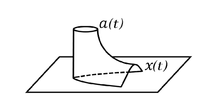
For and define the manifold of chimneys as:
(see Figure 8). For generic choices, is a smooth manifold of dimension , where denotes the Conley-Zehnder index of a loop .
Define
| (42) | ||||
It holds , hence is well defined on the homology level:
Let be a periodic orbit. If there exists , let be a periodic orbit defined as
Since , we have . Therefore, we have
so
It follows that defines the mapping
which also descends to the homology level:
(see also [10]). The diagram
| (43) |
commutes.
Similarly, set
and define
For generic choices, is a smooth manifold of dimension .
Define
This homomorphism also descends to the homology level
since it commutes with the boundary operators. As above, one can show that it also induces a homomorphism on the filtered homology level, and that the corresponding diagram (analogous to (43)) commutes.
Let (see Definition 4 on page • ‣ 4). We extend to in the following way. Consider a tubular neighbourhood of . First, we extend to the vector bundle over , and obtain the Morse function such that
Then we extend the Morse function defined on the open subset to the Morse function on such that there are no trajectories for the negative gradient flow of leaving (see [35] for details). Now the Morse complex is a subset of the Morse complex and the inclusion map of these complexes becomes the homomorphism on the homology level.
Proposition 25.
Let , and be as above. Let be a Hamiltonian. Suppose all the choices are generic. The diagram
| (44) |
commutes.
Proof: The upper diagram is (43). The lower diagram is
| (45) |
and its commutativity means that is holds
In order to do that using the usual cobordism arguments, we consider the following two auxiliary manifolds.
For let be a smooth cut-off function with the properties:
Let be the critical point of a Morse function and the critical point of a Morse function . Fix and define
(see Figure 9).
Define also
For and generic choices, is a smooth one-dimensional manifold with topological boundary that can be identified with
where
Here
i.e. it is the space of combined object defining a isomorphism for periodic orbits and .
The boundary components and correspond to the boundary of (since ). The boundary parts and come from the coordinate, and corresponds to the case . As regards the component , it arises when . More precisely, for
we define (for ):
| (46) |
and the approximative solution from Floer’s gluing construction to be:
In the equation (46) is a smooth cut-off function equal to for and to for . Vector fields are chosen such that
and are chosen similarly. The rest of the proof of Floer gluing theorem is standard.
Denote by the homomorphism obtained by counting the elements of the zero dimensional manifold . Since the number of the boundary of the one-dimensional manifold is even, i.e. zero in , and the maps and are of the form
the homomorphisms and are equal in the homology. By standard cobordism argument one can show that the mapping does not depend on . Now as in the proof of Theorem 9, we conclude that is chain homotopic to the map defined by the number of pairs with properties:
Since , is a negative gradient trajectory of connecting two critical points of the same Morse index. Thus, is chain homotopic to the homomorphism . On the other hand, the mapping is exactly the homomorphism , so the claim follows.
∎
We intend to compare spectral invariants for two Floer homologies. Since in Lagrangian case we are dealing with the direct limit construction, i.e. we have the whole family of Floer homology groups (for the approximations) to start with, we need to have the corresponding family in periodic orbits case, to maintain the transversality conditions. In periodic orbit case, the canonical isomorphisms for two different almost complex structures will be the homomorphisms that define a direct limit Floer homology group.
For two generic almost complex structures and , denote by a canonical isomorphism of Floer homologies for periodic orbits:
that satisfies
As before, define Floer homology for periodic orbits as a direct limit
The filtered Floer homology is defined as:
Proposition 26.
Let stands for a homomorphism (42) for the almost complex structure . We use the abbreviations
The diagram:
| (47) |
commutes.
Proof. The commutativity of (47) is equivalent to:
The proof of the above equality is similar to the proofs of the Proposition 11 and Lemma 15. The auxiliary one-dimensional manifold will be the set of the pairs , where , and is a chimney with the properties depicted in Figure 10. ∎
Corollary 27.
The following corollary follows from the commutativity of (44) for all the approximations.
Corollary 28.
The diagram
| (48) |
commutes.∎
Theorem 29.
Let . Then
One can obtain the inequality of similar type by using the homomorphism . The corresponding commutative diagram is
where is the map obtained by inclusion map and Poincaré duality map:
From this commutativity, we have the following
Theorem 30.
Let , then
Proof is analogous to this of Theorem 29.∎
4.6. A remark on invariants for subsets
In [29] Oh considered a spectral invariant
(the notions are the same as in the Subsection 4.1). If are two open subset of and
is surjective, Oh proved that
We can prove slightly more precise statement, the inequality for any homology class (with coefficients), using the PPS isomorphism for an open subset in the proof.
Theorem 31.
Let be two open subset of and let
(the homomorphism induced by inclusion ) be surjective. Let be as in (33). For it holds:
Proof: Let
denote the inclusion homomorphisms defined by Oh in [29]. The following diagram is commutative:
| (49) |
The commutativity of the upper diagram is proven in [29]. To prove the commutativity of the lower one, it is enough to prove the commutativity of
for all close enough to and close enough to . Here is the inclusion map also defined in [29]. Take in . It holds
| (50) |
On the other hand, we have
which is the same as (50) if is surjective.
Let
If , then , for , so, from the commutativity of (49) we have
We conclude that , therefore
so by taking an infimum over , we obtain
∎
References
- [1] A. Abbondadolo, M. Schwarz, Notes on Floer homology and loop space homology, Morse theoretic methods in nonlinear analysis and in symplectic topology, NATO Sci. Ser, II Math. Phys. Chem., vol. 217, Springer, Dordrecht, pp. 74–108, 2006.
- [2] A. Abbondandolo, M. Schwarz, Floer homology of cotangent bundles and the loop product, Geom. Topol., 14(3): 1569–1722, 2010.
- [3] P. Albers, A Lagrangian Piunikhin-Salamon-Schwarz morphism and two comparison homomorphisms in Floer homology , Int. Math. Res. Not. IMRN , no. 4, 56pp, 2008.
- [4] M. Audin, M. Damian, Morse theory and Floer homology, Springer Verlag, 2014.
- [5] D. Auroux, A beginner’s introduction to fukaya categories, arXiv:1301.7056, 2013.
- [6] M. Chaperon, Une idée du type ”géodésiques brisées” pur les systèmes hamiltoniens, C. R. Acad. Sc. Paris, 298, 293–296, 1984.
- [7] M. Chaperon, An elementary proof of the Conley-Zehnder theorem in symplectic geometry, In Braaksma, Broer, and Takens, editors, Dynamical Systems and Bifurcations, volume 1125 of Springer Lecture Notes in Mathematics, pages 1–8, 1985.
- [8] Y. Chekanov, Hofer’s symplectic energy and Lagrangian intersections, Publ. Newton Inst., Cambridge University Press 8, 296–306, 1996.
- [9] J. -Duretić, Piunikhin-Salamon-Schwarz isomorphisms and spectral invariants for conormal bundle, preprint, arXiv:1411.0852, 2014.
- [10] J. -Duretić, J. Katić, D. Milinković, Comparison of spectral invariants in Lagrangian and Hamiltonian Floer theory, Filomat, 30, no. 5, 1161–1174, 2016.
- [11] Y. Eliashberg, L. Polterovic, Symplectic quasi-states on the quadric surface and Lagrangian submanifolds, ArXiv:1006.2501v1, 2010.
- [12] U. Frauenfelder, F. Schlenk, Hamiltonian dynamics on convex symplectic manifolds, Israel J. Math., 159 1–56, 2007.
- [13] V. Humilière, R. Leclercq, S. Seyfaddini Coisotropic rigidity and symplectic geometry, ArXiv:1305.1287v2, 2015.
- [14] R. Kasturirangan, Y.-G. Oh, Quantization of Eilenberg–Steenrod axioms via Fary functors, RIMS preprint, 2000.
- [15] R. Kasturirangan, Y.-G. Oh, Floer homology for open subsets and a relative version of Arnold’s conjecture, Math. Z. 236, 151–189, 2001.
- [16] J. Katić, D. Milinković, Piunikhin-Salamon-Schwarz isomorphisms for Lagrangian intersections, Differential Geom. Appl. 22, no. 2, 215–227, 2005.
- [17] J. Katić, D. Milinković, T. Simčević, Isomorphism between Morse nad Lagrangian Floer cohomology rings, Rocky Mountain J. Math., 41, no.3, 789–811, 2011.
- [18] S. Lanzat, Hamiltonian Floer homology for compact convex symplectic manifolds, arXiv:1302.1025, 2015.
- [19] F. Laudenbach, J.-C. Sikorav, Persistence d’intersections avec la section nulle au conours d’une isotopie Hamiltonienne dans un fibre cotangent, Invent. Math., 82, 349–357, 1985.
- [20] R. Leclercq, Spectral invariants in Lagrangian Floer theory, J. Modern Dynamics 2, 249–286, 2008.
- [21] D. Milinković, Morse homology for generating functions of Lagrangian submanifolds, Trans. Amer. Math. Soc., Vol. 351, no. 10, 3953–3974, 1999.
- [22] ———–, On equivalence of two constructions of invariants of Lagrangian submanifolds, Pacific J. Math., Vol. 195, no. 2, 371–415, 2000.
- [23] ———–, Geodesics on the space of Lagrangian submanifolds in cotangent bundles, Proc. Amer. Math. Soc., 129 , 1843-1851, 2001.
- [24] ———–, Action spectrum and Hofer’s distance between Lagrangian submanifolds, Differential Geom. Appl., 17, 69-81, 2002.
- [25] J. Milnor, Lectures on the h-cobordism Theorem, Princeton University Press, 1963.
- [26] A. Monzner, N. Vichery, F. Zapolsky, Partial quasi-morphisms and quasi-states on cotangent bundles, and symplectic homogenization, Journal of Modern Dynamics, Issue 2, 205–-249, 2012.
- [27] Y.-G. Oh, Symplectic topology as the geometry of action functional I – relative Floer theory on the cotangent bundle, J. Differential Geom. 45, 499–577, 1997.
- [28] Y.-G. Oh, Symplectic topology as the geometry of action functional II – pants product and cohomological invariants, Comm. Anal. Geom. 7, 1–55, 1999.
- [29] Y.-G. Oh, Naturality of Floer homology of open subsets in Lagrangian intersection theory, in “Proc. of Pacific Rim Geometry Conference 1996”, International Press, pp. 261–280, 1998.
- [30] Y.-G. Oh, Geometry of generating functions and Lagrangian spectral invariants, arXiv:1206.4788, 2013.
- [31] S. Piunikhin, D. Salamon, M. Schwarz, Symplectic Floer–Donaldson theory and quantum cohomology, in: Contact and symplectic geometry, Publ. Newton Instit. 8, Cambridge Univ. Press, Cambridge, pp. 171–200, 1996.
- [32] L. Polterovich, D. Rosen Function theory on symplectic manifolds, CRM Monograph series, Volume 34, 2014.
- [33] J. Robbin, D. Salamon, The Maslov index for paths, Topology 32, 827–844, 1993.
- [34] J. Robbin, D. Salamon, The spectral flow and the Maslov index, Bull. London Math. Soc. 27, 1–33, 1995.
- [35] M. Schwarz, Morse Homology, Birkhäuser, 1993.
- [36] M. Schwarz. On the action spectrum for closed symplectically aspherical manifolds, Pacific J. Math., Vol. 193, no. 2, 419–461, 2000.
- [37] C. Viterbo, Symplectic topology as the geometry of generating functions, Math. Ann., 292(4), 685–710, 1992.