Stagnation of block GMRES and its relationship to block FOM

Abstract

We analyze the the convergence behavior of block GMRES and characterize the phenomenon of stagnation which is then related to the behavior of the block FOM method. We generalize the block FOM method to generate well-defined approximations in the case that block FOM would normally break down, and these generalized solutions are used in our analysis. This behavior is also related to the principal angles between the column-space of the previous block GMRES residual and the current minimum residual constraint space. At iteration $j$, it is shown that the proper generalization of GMRES stagnation to the block setting relates to the columnspace of the $j$th block Arnoldi vector. Our analysis covers both the cases of normal iterations as well as block Arnoldi breakdown wherein dependent basis vectors are replaced with random ones. Numerical examples are given to illustrate what we have proven, including a small application problem to demonstrate the validity of the analysis in a less pathological case.

65F10, 65F50, 65F08

1 Introduction

The Generalized Minimum Residual Method (GMRES) [31] and the Full Orthogonalization Method (FOM) [29] are two Krylov subspace methods for solving linear systems with non-Hermitian coefficient matrices and one right hand side, i.e.,

(1) $$\mathbf{A}\mathbf{x}=\mathbf{b}\mbox{\ \ \ with\ \ \ }\mathbf{A}\in\mathbb{C}^{n\times n}\mbox{\ \ \ and\ \ \ }\mathbf{b}\in\mathbb{C}^{n}.$$

The convergence behavior of these two methods is closely related, and this relationship was characterized by Brown [5], and other related results can be found in [7, 8, 38], and a related detailed geometric analysis of projection methods was presented in [10]. A nice description can also be found in [30, Section 6.5.5]. Krylov subspace methods have been generalized to treat the situation in which we have multiple right-hand sides, i.e., we are solving

(2) $$\mathbf{A}\mathbf{X}=\mathbf{B}\mbox{\ \ \ with\ \ \ }\mathbf{B}\in\mathbb{C}^{n\times L}.$$

In particular, block GMRES and block FOM [30, Section 6.12] have been proposed for solving (2); however, to our knowledge, a similar full analysis of block GMRES, the connection between stagnation and block FOM convergence, and accompanying geometric considerations have yet to be described in the literature. Therefore, in this work we analyze the stagnation behavior of block GMRES and characterize its relationship to the behavior of the block FOM method. Similar analytic tools as in in [5] and [10] are used, but the behavior of block methods is a bit more complicated to describe. The key result is the proper generalization of GMRES stagnation to the block setting. The analog of stagnation for block GMRES is not simply stagnation of some columns of the iterate. Rather, at iteration $j$ it is associated to the dimension of the intersection between the column space of the $j$th block Arnoldi vector and the $j$th block GMRES correction. Stagnation of some columns of the iterate is shown to be a special case thereof. This then allows analogs of many of the results on stagnation of GMRES and the relationship between GMRES and FOM to be proven in the block setting. As block methods can suffer from partial or full stagnation of the iteration and breakdowns due to linear dependence of the block residual, additional analysis is needed to fully characterize the stagnation in these settings. Here we consider the case that dependent basis vectors are replaced with random ones (as in [3, 6, 26, 36]). One could similarly consider the case that dependent vectors are removed and the block size reduced; see, e.g., [1, 20, 28, 24].

The rest of this paper proceeds as follows. In the next section, we review Krylov subspace methods, focusing in particular on block GMRES and block FOM. We also review existing analysis relating GMRES- and FOM-like methods. The type of relationship illuminated in [5] has been extended to many other pairs of methods. In Section 3, we present our main results which characterize the relationship between block GMRES and block FOM. In Section 4, we construct numerical examples which demonstrate what has been revealed by our analysis. We offer some discussion and conclusions in Section 5.

In this paper, we adopt the convention that $\mathbf{I}$ is the identity matrix, where context determines the appropriate dimension. When needed, we specify the dimension $\mathbf{I}_{J}\in\mathbb{R}^{J\times J}$. Similarly, $\mathbf{0}$ denotes the matrix of zeros, with dimension determined by context. We denote $\mathbf{0}_{J}\in\mathbb{R}^{J\times J}$ to be a square matrix of zeros and $\mathbf{0}_{J_{1}\times J_{2}}\in\mathbb{R}^{J_{1}\times J_{2}}$ with $J_{1}\neq J_{2}$ to be a rectangular matrix of zeros.

2 Background

In this section, we review the basics about Krylov subspace methods and focus on the the block version, designed to solve, e.g., (2). We describe everything in terms of block Krylov subspace methods, and discuss the simplifications in the case that the block size $L=1$. We then review existing results relating the iterates of pairs of methods (many times derived from Galerkin and minimum residual projections, respectively), e.g., FOM and GMRES [5] and BiCG and QMR [13] as well as subsequent works which expand upon and offer additional perspective on these pair-wise relationships, e.g., [7, 8, 16, 27, 38].

2.1 Single-vector and block Krylov subspaces

In the case that we are solving the system (2) with multiple right-hand sides (a block right-hand side), block Krylov subspace methods are an effective family of methods for generating high quality approximate solutions to (2) at relatively low cost. Let $\mathbf{X}_{0}$ be an initial approximate solution to (2) with block initial residual $\mathbf{F}_{0}~{}=~{}\mathbf{B}-\mathbf{A}\mathbf{X}_{0}$. We can define the $j$th block Krylov subspace as

(3) $$\mathbb{K}_{j}(\mathbf{A},\mathbf{F}_{0})=\rm span\left\{\mathbf{F}_{0},\mathbf{A}\mathbf{F}_{0},\mathbf{A}^{2}\mathbf{F}_{0},\ldots,\mathbf{A}^{j-1}\mathbf{F}_{0}\right\}$$

where the span of a collection of block vectors is understood to be the span of all their columns. When $L=1$ ($\mathbf{B},\,\mathbf{X}_{0}\in\mathbb{C}^{n}$), this definition reduces to the single-vector Krylov subspace, denoted ${\mathcal{K}}_{j}(\mathbf{A},\mathbf{F}_{0})$. In the case $L>1$, is straightforward to show that

$$\mathbb{K}_{j}(\mathbf{A},\mathbf{F}_{0})={\mathcal{K}}_{j}(\mathbf{A},\mathbf{F}_{0}(:,1))+{\mathcal{K}}_{j}(\mathbf{A},\mathbf{F}_{0}(:,2))+\cdots+{\mathcal{K}}_{j}(\mathbf{A},\mathbf{F}_{0}(:,L))$$

where we use the MATLAB style indexing notation $\mathbf{F}(:,i)$ to denote the $i$th column of a matrix $\mathbf{F}\in\mathbb{C}^{I\times J}$ such that $J\geq i$; see, e.g., [18].

Let $\mathbf{W}_{j}=\begin{bmatrix}\mathbf{V}_{1}&\mathbf{V}_{2}&\ldots\mathbf{V}_{j}\end{bmatrix}\in\mathbb{C}^{n\times jL}$ be the matrix with orthonormal columns spanning $\mathbb{K}_{j}(\mathbf{A},\mathbf{F}_{0})$ with $\mathbf{V}_{i}\in\mathbb{C}^{n\times L}$ having orthonormal columns, and $\mathbf{V}_{i}^{\ast}\mathbf{V}_{j}=\mathbf{0}$ for $i\neq j$. These orthonormal blocks can be generated one block at a time by an iterative orthogonalization process called the block Arnoldi process, which is a natural generalization of the Arnoldi process for the single-vector case. We have the block Arnoldi relation

(4) $$\mathbf{A}\mathbf{W}_{j}=\mathbf{W}_{j+1}\overline{\mathbf{H}}_{j}^{(B)}$$

where $\overline{\mathbf{H}}_{j}^{(B)}=\left(\mathbf{H}_{i,j}\right)\in\mathbb{C}^{(j+1)L\times jL}$ is block upper Hessenberg with $\mathbf{H}_{ij}\in\mathbb{C}^{L\times L}$ and $\mathbf{H}_{j+1,j}$ upper triangular.

We can derive block FOM and block GMRES methods through Galerkin and minimization constraints. We have for each column of the $j$th block residual the constraints

(5) $$\mathbf{R}_{j}(:,i) \perp \mathbb{K}_{j}(\mathbf{A},\mathbf{F}_{0})\mbox{\ \ \ or\ \ \ }$$

(6) $$\mathbf{R}_{j}(:,i) \perp \mathbf{A}\mathbb{K}_{j}(\mathbf{A},\mathbf{F}_{0}).$$

which lead to the block FOM and block GMRES methods, respectively. For both methods, approximations can be computed for all columns simultaneously. Let $\mathbf{X}_{j}^{(F)}$ and $\mathbf{X}_{j}^{(G)}$ denote the $j$th block FOM and block GMRES approximation solutions for (2). Furthermore, let $\mathbf{E}_{L}^{[I]}\in\mathbb{R}^{I\times L}$ have as columns the first $L$ columns of the $I\times I$ identity matrix, and let $\mathbf{F}_{0}=\mathbf{V}_{1}\mathbf{S}_{0}$ be the reduced QR-factorization with $\mathbf{S}_{0}\in\mathbb{C}^{L\times L}$ upper-triangular. Using (4), block FOM can be derived from (5) which leads to the formulation

(7) $$\mathbf{X}_{j}^{(F)}=\mathbf{X}_{0}+\mathbf{T}_{j}^{(F)}\mbox{\ \ \ where\ \ \ }\mathbf{T}_{j}^{(F)}=\mathbf{W}_{j}\mathbf{Y}_{j}^{(F)}\mbox{\ \ \ and\ \ \ }\mathbf{H}_{j}^{(B)}\mathbf{Y}_{j}^{(F)}=\mathbf{E}_{L}^{[jL]}\mathbf{S}_{0},$$

where $\mathbf{H}_{j}^{(B)}\in\mathbb{C}^{jL\times jL}$ is defined as the matrix containing the first $jL$ rows of $\overline{\mathbf{H}}_{j}^{(B)}$. Similarly for block GMRES, we can use (4), combined with (6) to yield a formulation

(8) $$\mathbf{X}_{j}^{(G)}=\mathbf{X}_{0}+\mathbf{T}_{j}^{(G)} \mathbf{T}_{j}^{(G)}=\mathbf{W}_{j}\mathbf{Y}_{j}^{(G)}$$    where

   and $$\mathbf{Y}_{j}^{(G)}=\underset{\mathbf{Y}\in\mathbb{C}^{jL\times L}}{\text{{\rm argmin}}}\left\|\overline{\mathbf{H}}_{j}^{(B)}\mathbf{Y}-\mathbf{E}_{L}^{[(j+1)L]}\mathbf{S}_{0}\right\|_{F},$$

where $\left\|\cdot\right\|_{F}$ is the Frobenius norm. Updates such as $\mathbf{T}_{j}^{(G)}$ and $\mathbf{T}_{j}^{(F)}$ are often called corrections and the subspaces from which they are drawn are called correction subspaces. There has been a great deal of research on the convergence properties of block methods such as block GMRES; see, e.g., [15, 21, 34].

In the case $L=1$, block Krylov methods reduce to the well-described single-vector Krylov subspace methods; see, e.g., [30, Section 6.3] and [35]. In this case, we drop the superscript $(B)$ and write $\overline{\mathbf{H}}_{j}:=\overline{\mathbf{H}}_{j}^{(B)}$. The block Arnoldi method simplifies to a simpler Gramm-Schmidt process in which the block entries $\mathbf{H}_{i,j}$ of $\overline{\mathbf{H}}_{j}$ reduce to scalars, now denoted with lower-case $h_{ij}\in\mathbb{C}$. Then using the scalar version of (4), single-vector FOM can be derived from (5) which leads to the formulation

$$\mathbf{x}_{j}^{(F)}=\mathbf{x}_{0}+\mathbf{t}_{j}^{(F)}\mbox{\ \ \ where\ \ \ }\mathbf{t}_{j}^{(F)}=\mathbf{V}_{j}\mathbf{y}_{j}^{(F)}\mbox{\ \ \ and\ \ \ }\mathbf{H}_{j}\mathbf{y}_{j}^{(F)}=\beta\mathbf{e}_{1}^{[j]},$$

where $\beta=\left\|\mathbf{F}_{0}\right\|$ is the $2$-norm of the single-vector residual, and $\mathbf{e}_{J}^{[I]}\in\mathbb{C}^{I}$ is the $J$th Cartesian basis vector in $\mathbb{C}^{I}$. Similarly for single-vector GMRES, we can use (4), combined with (6) to yield the formulation

$$\mathbf{x}_{j}^{(G)}=\mathbf{x}_{0}+\mathbf{t}_{j}^{(G)}\mbox{\ \ \ where\ \ \ }\mathbf{t}_{j}^{(G)}=\mathbf{V}_{j}\mathbf{y}_{j}^{(G)}\mbox{\ \ \ and\ \ \ }\mathbf{y}_{j}^{(G)}=\underset{\mathbf{y}\in\mathbb{C}^{j}}{\text{{\rm argmin}}}\left\|\overline{\mathbf{H}}_{j}\mathbf{y}-\beta\mathbf{e}_{1}^{[j+1]}\right\|.$$

In the case $L=1$, if at some iteration $j$ we have ${\mathcal{K}}_{j-1}(\mathbf{A},\mathbf{F}_{0})={\mathcal{K}}_{j}(\mathbf{A},\mathbf{F}_{0})$ (i.e., $\dim{\mathcal{K}}_{j}(\mathbf{A},\mathbf{F}_{0})=j-1<j$), then we have reached an invariant subspace, and both GMRES and FOM will produce an exact solution at that iteration. In this case, $j-1$ is called the grade of the pair $\left(\mathbf{A},\mathbf{F}_{0}\right)$, denoted $\nu(\mathbf{A},\mathbf{F}_{0})$. This notion of grade has been extended to the case $L>1$ [18]; however, the situation is a bit more complicated. It can occur that $\dim\mathbb{K}_{j}(\mathbf{A},\mathbf{F}_{0})<jL$ without convergence for all right-hand sides (in other words, without having reached the block grade of $\mathbf{A}$ and $\mathbf{F}_{0}$, the iteration at which we reach an invariant subspace). It may be that we have convergence for some or no right-hand sides. In this case, dependent block Arnoldi vectors are generated and there must be some procedure in place to gracefully handle this situation for reasons of stability. The dependence of block Arnoldi vectors and methods for handling this dependence have been discussed extensively in the literature; see, e.g., [3, 12, 15, 18, 22, 24, 32, 36], and general convergence analysis of block methods has been presented in, e.g., [21, 34, 33]. In this paper, we consider only the case that dependent basis vectors are replaced with random vectors.

2.2 Relationships between pairs of projection methods

Pairs of methods such FOM and GMRES which are derived from a Galerkin and minimum residual projection, respectively, over the same space are closely related. The analysis of Brown [5] characterized this relationship in the case of FOM and GMRES when $L=1$. We state here a theorem encapsulating the results relevant to this work. First, though, note that in FOM at iteration $j$, we must solve a linear system involving $\mathbf{H}_{j}$. Thus, if $\mathbf{H}_{j}$ is singular, the $j$th FOM iterate does not exist. We define $\widetilde{\mathbf{x}}_{j}^{(F)}$ to be the generalized FOM approximation through

(9) $$\widetilde{\mathbf{x}}_{j}^{(F)}=\mathbf{x}_{0}+\widetilde{\mathbf{t}}_{j}^{(F)}\mbox{\ \ \ where\ \ \ }\widetilde{\mathbf{t}}_{j}^{(F)}=\mathbf{V}_{j}\widetilde{\mathbf{y}}_{j}^{(F)}\mbox{\ \ \ and\ \ \ }\widetilde{\mathbf{y}}_{j}^{(F)}=\mathbf{H}_{j}^{\dagger}\left(\beta\mathbf{e}_{1}^{[j]}\right),$$

where $\mathbf{H}_{j}^{\dagger}$ is the Moore-Penrose pseudoinverse of $\mathbf{H}_{j}$. In the case that $\mathbf{H}_{j}$ is nonsingular, we have that $\widetilde{\mathbf{x}}_{j}^{(F)}=\mathbf{x}_{j}^{(F)}$, but $\widetilde{\mathbf{x}}_{j}^{(F)}$ is well-defined in the case that $\mathbf{x}_{j}^{(F)}$ does not exist. In this case $\widetilde{\mathbf{y}}_{j}^{(F)}$ minimizes $\left\|\mathbf{H}_{j}\mathbf{y}-\beta\mathbf{e}_{1}^{[j]}\right\|$ and has minimum norm of all possible minimizers. The following theorem combines two results proven by Brown in [5].

Theorem 2.1.

The matrix $\mathbf{H}_{j}$ is singular (and thus $\mathbf{x}_{j}^{(F)}$ does not exist) if and only if GMRES stagnates at iteration $j$ with $\mathbf{x}_{j}^{(G)}=\mathbf{x}_{j-1}^{(G)}$. Furthermore, in the case that $\mathbf{H}_{j}$ is singular, we have $\widetilde{\mathbf{x}}_{j}^{(F)}=\mathbf{x}_{j}^{(G)}$.

Thus in the GMRES stagnation case, it is shown that the two methods are “equivalent”, if we consider the generalized formulation of FOM. However, the relationship persists in the case that $\mathbf{H}_{j}$ is nonsingular as show in, e.g., [30]. In the same text, the following proposition is also shown.

Proposition 2.2.

Let $\mathbf{x}_{j}^{(G)}$ and $\mathbf{x}_{j}^{(F)}$ be the the $j$th GMRES and FOM approximations to the solution of (1) over the correction subspace ${\mathcal{K}}_{j}(\mathbf{A},\mathbf{F}_{0})$. Then we can write $\mathbf{x}_{j}^{(G)}$ as the following convex combination,

(10) $$\mathbf{x}_{j}^{(G)}=c_{j}^{2}\mathbf{x}_{j}^{(F)}+s_{j}^{2}\mathbf{x}_{j-1}^{(G)}$$

where $s_{j}$ and $c_{j}$ are the $j$th Givens sine and cosine, respectively, obtained from annihilating the entry $h_{j+1,j}$ while forming the QR-factorization of $\overline{\mathbf{H}}_{j}$.

One proves this by studying the differences between the QR-factorizations of the rectangular $\overline{\mathbf{H}}_{j}\in\mathbb{C}^{(j+1)\times j}$ and square $\mathbf{H}_{j}\in\mathbb{C}^{j\times j}$ generated by the single-vector Arnoldi process. The relation (10) reveals information about GMRES stagnation and its relationship to FOM. If $\mathbf{x}_{j}^{(G)}=\mathbf{x}_{j-1}^{(G)}$, then we have that $c_{j}=0$ which implies that $\mathbf{H}_{j}$ is singular and $\mathbf{x}_{j}^{(F)}$ does not exist. In this case, (10) can be thought of as still valid, in the sense that $s_{j}=1$, and (10) reduces to $\mathbf{x}_{j}^{(G)}=\mathbf{x}_{j-1}^{(G)}$ if we replace $\mathbf{x}_{j}^{(F)}$ with $\widetilde{\mathbf{x}}_{j}^{(F)}$.

This characterization of the relationship is not only important for understanding how these two methods behave at each iteration. They also reveal that FOM can suffer from stability issues when GMRES is close to stagnation as the matrix $\mathbf{H}_{j}$ is nearly singular (poorly conditioned) in this case. Whereas the residual curve of GMRES is monotonically nonincreasing, we see spikes in the FOM residual norm corresponding to periods of near stagnation in the GMRES method. These so-called “peaks” of residual norms of FOM and their relation to “plateaus” of the residual norms of GMRES have been previously studied; see, e.g., [7, 8, 38, 39]. Of particular interest is the observation by Walker [38] that the GMRES method can be seen as the result of a “residual smoothing” of the FOM residual. Similar observations extend to other pairings, such as QMR and BiCG.

3 Main Results

When $L>1$, block GMRES and block FOM also fit into the framework of a Galerkin/minimization pairing. Thus, it is natural that stagnation of block GMRES and behavior of the block FOM algorithm would exhibit the same relationship, using a generalized block FOM iterate defined similar to (9). However, this interaction is more complicated for a block method. There are interactions between the different approximations to individual systems. As such, the generalization of stagnation to the block GMRES setting must be done correctly. We introduce two definitions.

Definition 3.1.

At iteration $j$, we call the situation in which $\mathbf{X}_{j}^{(G)}=\mathbf{X}_{j-1}^{(G)}$ total stagnation. We call the situation in which some columns of the block GMRES approximation have stagnated but not all columns partial stagnation. Let $\mathbb{I}$ denote an indexing set such that $\mathbb{I}\subsetneq\left\{1,2,\ldots,L\right\}$, and let $\overline{\mathbb{I}}=\left\{1,2,\ldots,L\right\}\setminus\mathbb{I}$. For $\mathbf{F}\in\mathbb{C}^{J\times L}$, let $\mathbf{F}\left(:,\mathbb{I}\right)\in\mathbb{C}^{J\times\left|\mathbb{I}\right|}$ have as columns those from $\mathbf{F}$ corresponding to indices in $\mathbb{I}$. Then partial stagnation refers to the situation in which we have

(11) $$\mathbf{X}_{j}^{(G)}\left(:,\mathbb{I}\right)=\mathbf{X}_{j-1}^{(G)}\left(:,\mathbb{I}\right)\mbox{\ \ \ but \ \ }\mathbf{X}_{j}^{(G)}\left(:,i\right)\neq\mathbf{X}_{j-1}^{(G)}\left(:,i\right)\mbox{\ \ \ for each\ \ \ }i\in\overline{\mathbb{I}}.$$

Total stagnation is analogous to stagnation of GMRES in the single-vector case, as characterized in [5], but partial stagnation has no single-vector analog. Both total and partial stagnation can occur for multiple reasons. Total block GMRES stagnation can occur when block GMRES has converged, i.e., $\mathbf{X}_{j}^{(G)}=\mathbf{X}$, implying (if $j$ is the first iteration for which this occurs) from [18, Theorem 9], that we have that $j=\nu(\mathbf{A},\mathbf{F}_{0})$ and $\dim\mathbb{K}_{j+k}(\mathbf{A},\mathbf{F}_{0})=\dim\mathbb{K}_{j}(\mathbf{A},\mathbf{F}_{0})$ for all $k>0$. This case is trivial and will not be considered. If there is no breakdown of the block Arnoldi process (the rank of the block residual is $L$), then an occurrence of total stagnation is the block analog of single-vector GMRES stagnation. We prove in this case that Theorem 2.1 has a block analog; c.f., Corollary 3.17 and Corollary 3.20.

Partial stagnation has no direct analog to the single-vector case. Partial stagnation can occur when for column $i$, the system is exactly solved with $\mathbf{X}_{j}^{(G)}(:,i)=\mathbf{X}(:,i)$. This implies that $\mathbf{F}_{0}(:,i)-\mathbf{A}\mathbf{W}_{j}\mathbf{Y}_{j}^{(G)}(:,i)=0$, which implies that

$$\dim\left({\mathcal{R}}(\mathbf{F}_{0})\cap\mathbf{A}\mathbb{K}_{j}(\mathbf{A},\mathbf{F}_{0})\right)=1$$

(see, e.g., [28]) and that a dependent Arnoldi vector has been produced. In this case, one can treat this with one of the referenced strategies; see, e.g., [24, 3, 2, 4, 12, 37].

This is a specific instance of block Arnoldi process breakdown. At iteration $j$, the process breaks down when the matrix $\begin{bmatrix}\mathbf{B}&\mathbf{A}\mathbf{B}&\cdots&\mathbf{A}^{j-1}\mathbf{B}\end{bmatrix}$ is rank deficient which is equivalent to saying $\dim\left({\mathcal{R}}(\mathbf{X})\cap\mathbb{K}_{j}(\mathbf{A},\mathbf{F}_{0})\right)=\dim{\mathcal{N}}(\mathbf{R}_{j})>0$. In this case, $\mathbb{K}_{j}\left(\mathbf{A},\mathbf{F}_{0}\right)$ contains a linear combination of the columns of $\mathbf{X}$ [23, 28]. It has also been observed [28] that a dependent Arnoldi vector can be generated without the convergence of any of the columns.

In the case that there has been no breakdown of the block Arnoldi process we show that partial stagnation is actually a special case of a more general situation in which a part of the Krylov subspace does not contribute to the GMRES minimization process and the dimension of this subspace corresponds to the dimension of the null space of the rank-deficient FOM matrix $\mathbf{H}^{(B)}_{j}$; c.f., Theorem 3.16 and Theorem 3.19 below.

We derive a relationship for block GMRES and block FOM which is a generalization of (10) and is valid even in the case that $\mathbf{H}_{j}^{(B)}$ is singular. Thus, as in (9), we generalize the definition of the block FOM approximation to be compatible with a singular $\mathbf{H}_{j}^{(B)}$, i.e.,

(12) $$\widetilde{\mathbf{X}}_{j}^{(F)}=\mathbf{X}_{0}+\widetilde{\mathbf{T}}_{j}^{(F)} \widetilde{\mathbf{T}}_{j}^{(F)}=\mathbf{W}_{j}\widetilde{\mathbf{Y}}_{j}^{(F)}$$    where

   and $$\widetilde{\mathbf{Y}}_{j}^{(F)}=\left(\mathbf{H}_{j}^{(B)}\right)^{\dagger}\left(\mathbf{E}_{L}^{[jL]}\mathbf{S}_{0}\right)$$

where $\left(\mathbf{H}_{j}^{(B)}\right)^{\dagger}$ is the Moore-Penrose pseudoinverse of $\mathbf{H}_{j}^{(B)}$. In the case that $\mathbf{H}_{j}^{(B)}$ is nonsingular, we have that $\widetilde{\mathbf{X}}_{j}^{(F)}=\mathbf{X}_{j}^{(F)}$, but $\widetilde{\mathbf{X}}_{j}^{(F)}$ is well-defined in the case that $\mathbf{X}_{j}^{(F)}$ does not exist. In this case $\widetilde{\mathbf{Y}}_{j}^{(F)}$ minimizes $\left\|\mathbf{H}_{j}^{(B)}\mathbf{Y}-\mathbf{E}_{L}^{[jL]}\mathbf{S}_{0}\right\|_{F}$ and has minimum norm of all possible minimizers. As in (9), this definition reduces to the standard formulation of the FOM approximation in the case that $\mathbf{H}_{j}^{(B)}$ is nonsingular. In the single-vector case, to prove [30, Lemma 6.1], expressions are derived for the inverses of upper-triangular matrices. We need to obtain similar identities here. However, we want our derivation to be compatible with the case that $\mathbf{H}_{j}^{(B)}$ is singular.

To characterize both types of stagnation requires us to follow the work in [5], generalizing to the block Krylov subspace case. We also need to generalize (10) to the block GMRES/FOM setting. This is quite useful in extending the work in [5] and also of general interest.

3.1 GMRES and FOM from a particular perspective

We discuss briefly the known results for the relationship of single-vector GMRES and (generalized) FOM. This discussion closely relates to the discussion and results on ascent directions in, e.g., [5]. It has been shown that at the $j$th iteration the approximations $\mathbf{x}_{j}^{(G)}$ and $\widetilde{\mathbf{x}}_{j}^{(F)}$ can both be related to the $(j-1)st$, with

(13) $$\mathbf{x}_{j}^{(G)}=\mathbf{x}_{j-1}^{(G)}+\mathbf{s}_{j}^{(G)} \widetilde{\mathbf{x}}_{j}^{(F)}=\mathbf{x}_{j-1}^{(G)}+\widetilde{\mathbf{s}}_{j}^{(F)}$$    and

$$\mbox{\ \ \ where\ \ \ }\mathbf{s}_{j}^{(G)}=\mathbf{V}_{j}\mathbf{y}^{(G)}_{\mathbf{s}_{j}}\in{\mathcal{K}}_{j}(\mathbf{A},\mathbf{F}_{0}) \widetilde{\mathbf{s}}_{j}^{(F)}=\mathbf{V}_{j}\widetilde{\mathbf{y}}_{\mathbf{s}_{j}}^{(F)}\in{\mathcal{K}}_{j}(\mathbf{A},\mathbf{F}_{0})$$    and

where $\widetilde{\mathbf{y}}_{\mathbf{s}_{j}}^{(F)}$ and $\mathbf{y}^{(G)}_{\mathbf{s}_{j}}$ are representations of the generalized FOM and GMRES progressive corrections from ${\mathcal{K}}_{j}(\mathbf{A},\mathbf{F}_{0})$. The next proposition follows directly.

Proposition 3.2.

The GMRES and generalized FOM updates $\mathbf{y}^{(G)}_{\mathbf{s}_{j}}$ and $\widetilde{\mathbf{y}}_{\mathbf{s}_{j}}^{(F)}$ respectively satisfy the minimizations

(14) $$\mathbf{y}^{(G)}_{\mathbf{s}_{j}} = \underset{\mathbf{y}\in\mathbb{C}^{n}}{\text{{\rm argmin}}}\left\|\begin{bmatrix}\beta\mathbf{e}_{1}^{[j]}-\overline{\mathbf{H}}_{j-1}\mathbf{y}_{j-1}^{(G)}\\ 0\end{bmatrix}-\overline{\mathbf{H}}_{j}\mathbf{y}\right\|\mbox{\ \ \ and\ \ \ }$$

(15) $$\widetilde{\mathbf{y}}_{\mathbf{s}_{j}}^{(F)} = \underset{\mathbf{y}\in\mathbb{C}^{n}}{\text{{\rm argmin}}}\left\|\beta\mathbf{e}_{1}^{[j]}-\overline{\mathbf{H}}_{j-1}\mathbf{y}_{j-1}^{(G)}-\mathbf{H}_{j}\mathbf{y}\right\|.$$

Proof.  To prove (14), one simply inserts the expression for $\mathbf{x}_{j}^{(G)}$ from (13) into the residual and applies the GMRES Petrov-Galerkin condition (6). To prove (15), one begins similarly, by substituting the expression for $\mathbf{x}_{j}^{(F)}$ from (13) into the residual and applying the FOM Galerkin condition (5). In this case, if $\mathbf{H}_{j}$ is nonsingular, this is equivalent to solving the linear system

(16) $$\mathbf{H}_{j}\widetilde{\mathbf{y}}_{\mathbf{s}_{j}}^{(F)}=\beta\mathbf{e}_{1}^{[j]}-\overline{\mathbf{H}}_{j-1}\mathbf{y}_{j}^{(G)}.$$

In the case that $\mathbf{H}_{j}$ is singular (the $j$th FOM approximation does not exist), we set

(17) $$\widetilde{\mathbf{y}}_{\mathbf{s}_{j}}^{(F)}=\mathbf{H}_{j}^{\dagger}\left(\beta\mathbf{e}_{1}^{[j]}-\overline{\mathbf{H}}_{j-1}\mathbf{y}_{j}^{(G)}\right).$$

In either case, we have that $\widetilde{\mathbf{y}}_{\mathbf{s}_{j}}^{(F)}$ is the minimizer of (15), yielding the result.         The result on FOM is [5, Theorem 3.3] but stated differently. This formulation allows us to discuss the GMRES and FOM at iteration $j$ using the $(j-1)$st GMRES minimization. We see that the GMRES method least-squares problem simply grows by one dimension when we go from iteration $j-1$ to $j$. However, at iteration $j$, imposing the FOM Galerkin condition (5) is equivalent to an augmentation of the $(j-1)$st GMRES least squares matrix. This augmented matrix is square. If it is nonsingular, then the $j$th FOM approximation exists and we solve the augmented system (16). If the augmented matrix is singular, then the generalized FOM approximation is computed by solving the least squares problem (17). In the case of single-vector GMRES and FOM, this is not necessary to characterize their relationship. However, in the case of block GMRES and block FOM, we can better discuss a generalization to the more complicated block Krylov subspace situation.

3.2 The QR-Factorization of the block upper Hessenberg matrices

We begin by describing the structure of the QR-factorizations of the square and rectangular block Hessenberg matrices.

Lemma 3.3.

Let $\overline{\mathbf{R}}_{j}\in\mathbb{C}^{j+1\times j}$ and $\widehat{\mathbf{R}}_{j}\in\mathbb{C}^{j\times j}$ be the R-factors of the respective QR-factorizations of $\overline{\mathbf{H}}_{j}^{(B)}$ and $\mathbf{H}_{j}^{(B)}$, and let $\mathbf{R}_{j}$ be the $j\times j$ non-zero block of $\overline{\mathbf{R}}_{j}$. Then $\overline{\mathbf{R}}_{j}$ and $\widehat{\mathbf{R}}_{j}$ both have as their upper left $j-1\times j-1$ block the R-factor of the QR-factorization of $\overline{\mathbf{H}}_{j-1}^{(B)}$, i.e., $\mathbf{R}_{j-1}$. Furthermore, the structures of $\overline{\mathbf{R}}_{j}$ and $\widehat{\mathbf{R}}_{j}$, respectively, are,

(18) $$\overline{\mathbf{R}}_{j}=\begin{bmatrix}\mathbf{R}_{j-1}&\mathbf{Z}_{j}\\ &\mathbf{N}_{j}\\ &\end{bmatrix}\mbox{\ \ \ and\ \ \ }\widehat{\mathbf{R}}_{j}=\begin{bmatrix}\mathbf{R}_{j-1}&\mathbf{Z}_{j}\\ &\widehat{\mathbf{N}}_{j}\end{bmatrix},$$

where $\mathbf{Z}_{j}\in\mathbb{C}^{(j-1)L\times L}$ and $\mathbf{N}_{j},\widehat{\mathbf{N}}_{j}\in\mathbb{C}^{L\times L}$ are upper triangular.

Proof.  Let $\mathbf{Q}_{i}^{(j+1)}\in\mathbb{C}^{j+1\times j+1}$ be orthonormal transformation which annihilates all subdiagonal entries in columns $i-1+1$ to $i$ of $\overline{\mathbf{H}}_{j}^{(B)}$ and effects no other rows so that we can write

$$\mathbf{Q}_{j-1}^{(j+1)}\cdots\mathbf{Q}_{1}^{(j+1)}\overline{\mathbf{H}}_{j}^{(B)}=\begin{bmatrix}\mathbf{R}_{j-1}&\mathbf{Z}_{j}\\ &\widehat{\mathbf{H}}_{j,j}\\ &\mathbf{H}_{j+1,j}\end{bmatrix}\mbox{\ \ \ and\ \ \ }\mathbf{Q}_{j-1}^{(j)}\cdots\mathbf{Q}_{1}^{(j)}\mathbf{H}_{j}^{(B)}=\begin{bmatrix}\mathbf{R}_{j-1}&\mathbf{Z}_{j}\\ &\widehat{\mathbf{H}}_{j,j}\end{bmatrix}.$$

Let $\widehat{\mathbf{Q}}_{j}^{(j)}\in\mathbb{C}^{j\times j}$ be the orthogonal transformation which annihilate the lower subdiagonal entries the block $\widehat{\mathbf{H}}_{j,j}$ in $\mathbf{Q}_{j-1}^{(j)}\cdots\mathbf{Q}_{1}^{(j)}\mathbf{H}_{j}^{(B)}$ and effects no other rows. Then we have

(19) $$\overline{\mathbf{R}}_{j}=\mathbf{Q}_{j}^{(j+1)}\begin{bmatrix}\mathbf{R}_{j-1}&\mathbf{Z}_{j}\\ &\widehat{\mathbf{H}}_{j,j}\\ &\mathbf{H}_{j+1,j}\end{bmatrix}\mbox{\ \ \ and\ \ \ }\widehat{\mathbf{R}}_{j}=\widehat{\mathbf{Q}}_{j}^{(j)}\begin{bmatrix}\mathbf{R}_{j-1}&\mathbf{Z}_{j}\\ &\widehat{\mathbf{H}}_{j,j}\end{bmatrix},$$

and the Lemma is proven.         Thus, the two core problems which must be solved at every iteration of block GMRES and block FOM can be written

(20) $$\begin{bmatrix}\mathbf{R}_{j-1}&\mathbf{Z}_{j}\\ &\mathbf{N}_{j}\end{bmatrix}\mathbf{Y}_{j}^{(G)}=(\mathbf{Q}_{j}^{(j+1)}\cdots\mathbf{Q}_{1}^{(j+1)}\mathbf{E}_{j+1}^{[j+1]}\mathbf{S}_{0})_{1:j}$$

(21) $$\mbox{\ \ \ and\ \ \ }\begin{bmatrix}\mathbf{R}_{j-1}&\mathbf{Z}_{j}\\ &\widehat{\mathbf{N}}_{j}\end{bmatrix}\mathbf{Y}_{j}^{(F)}=\widehat{\mathbf{Q}}_{j}^{(j)}\mathbf{Q}_{j-1}^{(j)}\cdots\mathbf{Q}_{1}^{(j)}\mathbf{E}_{j}^{[j]}\mathbf{S}_{0}.$$

It is also straightforward to show that the block right-hand sides of these core problems are related. If

$$\mathbf{G}_{j}^{(G)}=(\mathbf{Q}_{j}^{(j+1)}\cdots\mathbf{Q}_{1}^{(j+1)}\mathbf{E}_{L}^{[j+1]}\mathbf{S}_{0})_{1:j}\mbox{\ \ \ and\ \ \ }\mathbf{G}_{j}^{(F)}=\widehat{\mathbf{Q}}_{j}^{(j)}\mathbf{Q}_{j-1}^{(j)}\cdots\mathbf{Q}_{1}^{(j)}\mathbf{E}_{L}^{[j+1]}\mathbf{S}_{0},$$

then $\mathbf{G}_{j}^{(G)}$ and $\mathbf{G}_{j}^{(F)}$ are equal for the first $j-1$ rows, with

(22) $$\mathbf{G}_{j}^{(G)}=\begin{bmatrix}\mathbf{G}_{j-1}^{(G)}\\ \mathbf{C}_{j}\end{bmatrix}\mbox{\ \ \ and\ \ \ }\mathbf{G}_{j}^{(F)}=\begin{bmatrix}\mathbf{G}_{j-1}^{(G)}\\ \widehat{\mathbf{C}}_{j}\end{bmatrix}$$

where we have that

(23) $$\mathbf{G}_{j}^{(G)}=\left(\mathbf{Q}_{j}^{(j+1)}\begin{bmatrix}\mathbf{G}_{j-1}^{(G)}\\ \widetilde{\mathbf{C}}_{j}\\ \mathbf{0}\end{bmatrix}\right)_{1:j}=\left(\begin{bmatrix}\mathbf{G}_{j-1}^{(G)}\\ {\mathbf{C}}_{j}\\ \boldsymbol{\ast}\end{bmatrix}\right)_{1:j}.$$

This is a consequence of the structure of the orthogonal transformations used to define these vectors. It is important to pause here for a moment to discuss the $L\times L$ matrices $\mathbf{C}_{j}$, $\widehat{\mathbf{C}}_{j}$, and $\widetilde{\mathbf{C}}_{j}$ and characterize if and when they are full rank. At times for convenience, we refer to these matrices as the “$\mathbf{C}$-matrices”.

Lemma 3.4.

We have that $\rm rank\ \widetilde{\mathbf{C}}_{j}=\rm rank\ \mathbf{F}_{j-1}^{(G)}$; and, in particular, if $\dim\mathbb{K}_{j-1}(\mathbf{A},\mathbf{F}_{0})=(j-1)L$, we have that, $\widetilde{\mathbf{C}}_{j}$ is nonsingular.

Proof.  Let $\mathbf{Y}_{j-1}^{(G)}$ be the solution to the block GMRES least squares subproblem (8) but for iteration $j-1$. Let

$$\mathbf{F}_{j-1}^{(G)}=\mathbf{B}-\mathbf{A}\mathbf{X}_{j-1}^{(G)}=\mathbf{W}_{j}\left(\overline{\mathbf{H}}_{j-1}\mathbf{Y}_{j-1}^{(G)}-\mathbf{E}_{L}^{[j]}\mathbf{S}_{0}\right).$$

By assumption (20) has a solution at iteration $j-1$, and thus

$$\overline{\mathbf{H}}_{j-1}\mathbf{Y}_{j-1}^{(G)}-\mathbf{E}_{L}^{[j]}\mathbf{S}_{0}=\mathbf{Q}_{j-1}^{\ast}\begin{bmatrix}\mathbf{G}_{j-1}^{(G)}\\ \mathbf{C}_{j}\\ \mathbf{0}\end{bmatrix}-\mathbf{E}_{L}^{[j]}\mathbf{S}_{0}.$$

where $\overline{\mathbf{Q}}_{j-1}=\mathbf{Q}_{j-1}^{(j)}\cdots\mathbf{Q}_{1}^{(j)}$. Since $\mathbf{W}_{j-1}$ and $\overline{\mathbf{Q}}_{j-1}$ are both full rank, we have

$$\rm rank\ \mathbf{F}_{j-1}^{(G)}=\rm rank\ \mathbf{Q}_{j-1}\mathbf{W}_{j}^{\ast}\mathbf{F}_{j}^{(G)}=\rm rank\ \left(\begin{bmatrix}\mathbf{G}_{j-1}^{(G)}\\ \mathbf{C}_{j-1}\\ \mathbf{0}\end{bmatrix}-\begin{bmatrix}\mathbf{G}_{j-1}^{(G)}\\ \mathbf{C}_{j-1}\\ \widetilde{\mathbf{C}}_{j}\end{bmatrix}\right) = \rm rank\ \begin{bmatrix}\mathbf{0}\\ \mathbf{0}\\ -\widetilde{\mathbf{C}}_{j}\end{bmatrix}$$

$$= \rm rank\ \widetilde{\mathbf{C}}_{j}.$$

If we assume that the block Arnoldi method has not produced any dependent basis vectors, then we know from [28, Section 2, Corollary 1] that $\mathbf{F}_{j-1}^{(G)}$ is full-rank meaning $\widetilde{\mathbf{C}}_{j}$ is nonsingular.        

From this, we can similarly characterize the ranks of ${\mathbf{C}}_{j}$ and $\widehat{\mathbf{C}}_{j}$ which are closely related to $\widetilde{\mathbf{C}}_{j}$.

Lemma 3.5.

We have that $\rm rank\ \widehat{\mathbf{C}}_{j}=\rm rank\ \widetilde{\mathbf{C}}_{j}$. In particular, if $\dim\mathbb{K}_{j-1}(\mathbf{A},\mathbf{F}_{0})=(j-1)L$, we have that $\widehat{\mathbf{C}}_{j}$ is square and nonsingular.

Proof.  Let $\widehat{\mathbf{Q}}_{j}^{(j)}=\begin{bmatrix}\mathbf{I}_{j-1}&\\ &\widehat{\mathbf{Q}}_{j}^{(b)}\end{bmatrix}$ where $\widehat{\mathbf{Q}}_{j}^{(b)}\in\mathbb{C}^{L\times L}$ is the orthogonal transformation such that the second equation of (19) holds. Then from (23), we have $\widehat{\mathbf{C}}_{j}=\widehat{\mathbf{Q}}_{j}^{(b)}\widetilde{\mathbf{C}}_{j}$. If $\widetilde{\mathbf{C}}_{j}$ has full rank, the second statement follows.        

We can prove a similar result for $\mathbf{C}_{j}$, which will be used later to verify the nonsingularity of $\mathbf{C}_{j}$ under certain conditions.

Lemma 3.6.

Let

$$\mathbf{Q}_{j}^{(j+1)}=\begin{bmatrix}\mathbf{I}_{{\mathcal{J}}(j-2)}&&\\ &\mathbf{Q}_{j}^{(11)}&\mathbf{Q}_{j}^{(11)}\\ &\mathbf{Q}_{j}^{(21)}&\mathbf{Q}_{j}^{(22)}\end{bmatrix}$$

with $\mathbf{Q}_{j}^{(11)}\in\mathbb{C}^{L\times L}$, $\mathbf{Q}_{j}^{(12)}\in\mathbb{C}^{L\times L}$, $\mathbf{Q}_{j}^{(21)}\in\mathbb{C}^{L\times L}$, and $\mathbf{Q}_{j}^{(22)}\in\mathbb{C}^{L\times L}$. In general, we have $rank\,\mathbf{C}_{j}\leq\min\left\{\rm rank\ \mathbf{Q}_{j}^{(11)},\rm rank\ \widetilde{\mathbf{C}}_{j}\right\}$. If $\dim\mathbb{K}_{j-1}(\mathbf{A},\mathbf{F}_{0})~{}=~{}(j~{}-~{}1)L$, we have $\mathbf{C}_{j}$ is singular if and only if $\mathbf{Q}_{j}^{(11)}$ is singular.

Proof.  From (23) we have that $\mathbf{C}_{j}=\mathbf{Q}_{j}^{(11)}\widetilde{\mathbf{C}}_{j}$. The general result comes from basic inequality results for ranks of products of matrices; see, e.g., [19, Chapter 0]. If we assume $\dim\mathbb{K}_{j-1}(\mathbf{A},\mathbf{F}_{0})~{}=~{}(j~{}-~{}1)L$, then we know that $\widetilde{\mathbf{C}}_{j}$ has full rank, and the second result (in both directions) follows.        

We see that the ranks of $\widetilde{\mathbf{C}}_{j}$ and $\widehat{\mathbf{C}}_{j}$ are directly connected to block Arnoldi breakdown at iteration $j-1$. Later in Section 3.3, we assume no breakdown, thus both $\widetilde{\mathbf{C}}_{j}$ and $\widehat{\mathbf{C}}_{j}$ are nonsingular. In Section 3.4, we assume that the block Arnoldi process produces dependent vectors at iteration $j$ which are replaced with random vectors. Thus, at iteration $j$, both $\widetilde{\mathbf{C}}_{j}$ and $\widehat{\mathbf{C}}_{j}$ are still nonsingular, and their dimensions do not change at subsequent iterations.

We now turn to solving (21) and either solving (20) or obtaining the generalized least squares solution if $\widehat{\mathbf{R}}_{j}$ is singular. Since $\mathbf{R}_{j}$ is nonsingular, we simply compute the actual inverse while for $\widehat{\mathbf{R}}_{j}$, we compute the pseudo-inverse. These are both straightforward generalizations of the identities used in the proof of [30, Lemma 6.1], though verifying the structure of the Moore-Penrose pseudo-inverse identity requires a bit of thought. Let us recall briefly the following definition which can be found in, e.g., [11, Section 2.2],

Definition 3.7.

Let $T:{\mathcal{X}}\rightarrow{\mathcal{Y}}$ be a bounded linear operator between Hilbert spaces. Let ${\mathcal{N}}(T)$ denote the null space and ${\mathcal{R}}(T)$ denote the range of $T$ and define $\widetilde{T}:{\mathcal{N}}(T)^{\perp}\rightarrow{\mathcal{R}}(T)$ to be the invertible operator such that $\widetilde{T}x=Tx$ for all $x~{}\in~{}{\mathcal{N}}(T)^{\perp}$. Then we call the operator $T^{\dagger}$ the Moore-Penrose pseudo-inverse if it is the unique operator satisfying

1. ${\left.\kern-1.2ptT^{\dagger}\vphantom{\big{|}}\right|_{{\mathcal{R}}(T)}}=\widetilde{T}^{-1}$

2. ${\left.\kern-1.2ptT^{\dagger}\vphantom{\big{|}}\right|_{{\mathcal{R}}(T)^{\perp}}}=0_{op}$

where $0_{op}$ is the zero operator.

This definition is more general than the matrix-specific definition given in, e.g., [14, Section 5.5.2]. We choose to follow Definition 3.7 as it renders the proof of the following lemma less dependent on many lines of block matrix calculations, but of course the theoretical results are the same.

Lemma 3.8.

The inverse and pseudo-inverse, respectively, of $\mathbf{R}_{j}$ and $\widehat{\mathbf{R}}_{j}$ can be directly constructed from the identities (18), i.e.,

(24) $$\mathbf{R}_{j}^{-1}=\begin{bmatrix}\mathbf{R}_{j-1}^{-1}&-\mathbf{R}_{j-1}^{-1}\mathbf{Z}_{j}\mathbf{N}_{j}^{-1}\\ &\mathbf{N}_{j}^{-1}\end{bmatrix}\mbox{\ \ \ and\ \ \ }\widehat{\mathbf{R}}_{j}^{\dagger}=\begin{bmatrix}\mathbf{R}_{j-1}^{-1}&-\mathbf{R}_{j-1}^{-1}\mathbf{Z}_{j}\widehat{\mathbf{N}}_{j}^{\dagger}\\ &\widehat{\mathbf{N}}_{j}^{\dagger}\end{bmatrix},$$

where $\widehat{\mathbf{N}}_{j}^{\dagger}$ is the Moore-Penrose pseudo-inverse of $\widehat{\mathbf{N}}_{j}$.

Proof.  The expression for $\mathbf{R}_{j}^{-1}$ can be directly verified by left and right multiplication. To verify the expression for $\widehat{\mathbf{R}}_{j}^{\dagger}$, we must verify the two conditions listed in Definition 3.7.

To verify Condition 1, we first construct a basis for ${\mathcal{N}}(\widehat{\mathbf{R}}_{j})$. Observe that under our assumption that $\mathbf{R}_{j-1}$ is nonsingular, we have that

$$\dim{\mathcal{N}}(\widehat{\mathbf{R}}_{j})=\dim{\mathcal{N}}(\widehat{\mathbf{N}}_{j})=L-r$$

where $r=\rm rank\ (\widehat{\mathbf{N}}_{j})$. Let $\left\{\mathbf{y}_{i}\right\}_{i=1}^{r}$ be a basis for ${\mathcal{N}}(\widehat{\mathbf{N}}_{j})^{\perp}$. Furthermore, let $\left\{\mathbf{m}_{i}\right\}_{i=1}^{j-1}$ be a basis for $\mathbb{R}^{j-1}$. Then it follows that

$$\left\{\begin{bmatrix}\mathbf{R}_{j-1}^{-1}\mathbf{m}_{1}\\ \mathbf{0}\end{bmatrix},\ldots,\begin{bmatrix}\mathbf{R}_{j-1}^{-1}\mathbf{m}_{j-1}\\ \mathbf{0}\end{bmatrix},\begin{bmatrix}-\mathbf{R}_{j-1}^{-1}\mathbf{Z}_{j}\mathbf{y}_{1}\\ \mathbf{y}_{1}\end{bmatrix},\ldots,\begin{bmatrix}-\mathbf{R}_{j-1}^{-1}\mathbf{Z}_{j}\mathbf{y}_{r}\\ \mathbf{y}_{r}\end{bmatrix}\right\}$$

is a basis for ${\mathcal{N}}(\widehat{\mathbf{R}}_{j})^{\perp}$. For any $\widehat{\mathbf{x}}\in{\mathcal{N}}(\widehat{\mathbf{R}}_{j})^{\perp}$, we can write

$$\widehat{\mathbf{x}}=\sum_{i=1}^{j-1}\alpha_{i}\begin{bmatrix}\mathbf{R}_{j-1}^{-1}\mathbf{m}_{i}\\ \mathbf{0}\end{bmatrix}+\sum_{i=1}^{r}\beta_{i}\begin{bmatrix}-\mathbf{R}_{j-1}^{-1}\mathbf{Z}_{j}\mathbf{y}_{i}\\ \mathbf{y}_{i}\end{bmatrix}.$$

By direct calculation, we see that

$$\widehat{\mathbf{R}}_{j}\widehat{\mathbf{x}}=\sum_{i=1}^{j-1}\alpha_{i}\begin{bmatrix}\mathbf{m}_{i}\\ \mathbf{0}\end{bmatrix}+\sum_{i=1}^{r}\beta_{i}\begin{bmatrix}\mathbf{0}\\ \widehat{\mathbf{N}}_{j}\mathbf{y}_{j}\end{bmatrix},$$

and applying our prospective pseudo-inverse yields

$$\widehat{\mathbf{R}}_{j}^{\dagger}\widehat{\mathbf{R}}_{j}\widehat{\mathbf{x}}=\sum_{i=1}^{j-1}\alpha_{i}\begin{bmatrix}\mathbf{R}_{j-1}^{-1}\mathbf{m}_{i}\\ \mathbf{0}\end{bmatrix}+\sum_{i=1}^{r}\beta_{i}\begin{bmatrix}-\mathbf{R}_{j-1}^{-1}\mathbf{Z}_{j}\widehat{\mathbf{N}}_{j}^{\dagger}\widehat{\mathbf{N}}_{j}\mathbf{y}_{i}\\ \widehat{\mathbf{N}}_{j}^{\dagger}\widehat{\mathbf{N}}_{j}\mathbf{y}_{i}\end{bmatrix}.$$

Finally, we observe that since $\left\{\mathbf{y}_{i}\right\}_{i=1}^{r}$ is a basis for ${\mathcal{N}}(\widehat{\mathbf{N}}_{j})^{\perp}$, we have from Definition 3.7 that $\widehat{\mathbf{N}}_{j}^{\dagger}\widehat{\mathbf{N}}_{j}\mathbf{y}_{i}~{}=~{}\mathbf{y}_{i}$ for all $i$, and thus $\widehat{\mathbf{R}}_{j}^{\dagger}\widehat{\mathbf{R}}_{j}\widehat{\mathbf{x}}=\widehat{\mathbf{x}}$, verifying Condition 1.

To verify Condition 2, we first observe that

$$\left\{\begin{bmatrix}\mathbf{m}_{1}\\ \mathbf{0}\end{bmatrix},\ldots,\begin{bmatrix}\mathbf{m}_{j-1}\\ \mathbf{0}\end{bmatrix},\begin{bmatrix}\mathbf{0}\\ \widehat{\mathbf{N}}_{j}\mathbf{y}_{1}\end{bmatrix},\ldots,\begin{bmatrix}\mathbf{0}\\ \widehat{\mathbf{N}}_{j}\mathbf{y}_{r}\end{bmatrix}\right\}$$

is a basis for ${\mathcal{R}}(\widehat{\mathbf{R}}_{j})$. Let $\left\{\mathbf{c}_{i}\right\}_{i=1}^{L-r}$ be a basis for ${\mathcal{R}}(\widehat{\mathbf{N}}_{j})^{\perp}$. Then it follows that $\left\{\begin{bmatrix}\mathbf{0}\\ \mathbf{c}_{i}\end{bmatrix}\right\}_{i=1}^{L-r}$ is a basis for ${\mathcal{R}}(\widehat{\mathbf{R}}_{j})^{\perp}$. Let $\tilde{\mathbf{y}}=\sum_{i=1}^{L-r}\gamma_{i}\begin{bmatrix}\mathbf{0}\\ \mathbf{c}_{i}\end{bmatrix}$ be an element of ${\mathcal{R}}(\widehat{\mathbf{R}}_{j})^{\perp}$. Then we have

$$\widehat{\mathbf{R}}_{j}^{\dagger}\tilde{\mathbf{y}}=\sum_{i=1}^{L-r}\gamma_{i}\begin{bmatrix}-\mathbf{R}_{j-1}^{-1}\mathbf{Z}_{j}\widehat{\mathbf{N}}_{j}^{\dagger}\mathbf{c}_{i}\\ \widehat{\mathbf{N}}_{j}^{\dagger}\mathbf{c}_{i}\end{bmatrix}.$$

It follows directly from Definition (3.7) that $\widehat{\mathbf{N}}_{j}^{\dagger}\mathbf{c}_{i}=0$ for all $i$, and this proves Condition 2, thus proving the the lemma.         The following corollary technically follows from Lemma 3.8, though it can easily be proven directly.

Corollary 3.9.

If $\mathbf{H}_{j}^{(B)}$ is nonsingular, then it follows that $\widehat{\mathbf{R}}_{j}^{-1}$ and can be written

$$\widehat{\mathbf{R}}_{j}^{-1}=\begin{bmatrix}\mathbf{R}_{j-1}^{-1}&-\mathbf{R}_{j-1}^{-1}\mathbf{Z}_{j}\widehat{\mathbf{N}}_{j}^{-1}\\ &\widehat{\mathbf{N}}_{j}^{-1}\end{bmatrix}.$$

Now we have all the pieces we need to analyze the relationship between the block GMRES and block FOM approximations, and we can then discuss the implications with respect to stagnation.

3.3 The case of a breakdown-free block Arnoldi process

We begin this section by discussing block GMRES and block FOM from the same perspective as advocated in Section 3.1. We have the block analog of Proposition 3.2, and in this case we explicitly construct the block analogs of $\mathbf{s}_{j}^{(G)}$ and $\mathbf{s}_{j}^{(F)}$.

Lemma 3.10.

Let $\mathbf{S}_{j}^{(G)}=\mathbf{W}_{j}\mathbf{Y}_{\mathbf{S}_{j}}^{(G)}$ and $\widetilde{\mathbf{S}}_{j}^{(F)}=\mathbf{W}_{j}\widetilde{\mathbf{Y}}_{\mathbf{S}_{j}}^{(F)}$ both be in $\mathbb{C}^{n\times L}$ such that they satisfy the block GMRES and FOM progressive update formulas

(25) $$\mathbf{X}_{j}^{(G)}=\mathbf{X}_{j-1}^{(G)}+\mathbf{S}_{j}^{(G)} \widetilde{\mathbf{X}}_{j}^{(F)}=\mathbf{X}_{j-1}^{(G)}+\widetilde{\mathbf{S}}_{j}^{(F)}.$$    and

Then we can write

(26) $$\mathbf{Y}_{\mathbf{S}_{j}}^{(G)}=\begin{bmatrix}-\mathbf{R}_{j-1}^{-1}\mathbf{Z}_{j}\mathbf{N}_{j}^{-1}\mathbf{C}_{j}\\ \mathbf{N}_{j}^{-1}\mathbf{C}_{j}\end{bmatrix}\mbox{\ \ \ and\ \ \ }\widetilde{\mathbf{Y}}_{\mathbf{S}_{j}}^{(F)}=\begin{bmatrix}-\mathbf{R}_{j-1}^{-1}\mathbf{Z}_{j}\widehat{\mathbf{N}}_{j}^{\dagger}\widehat{\mathbf{C}}_{j}\\ \widehat{\mathbf{N}}_{j}^{\dagger}\widehat{\mathbf{C}}_{j}\end{bmatrix},$$

and these vectors minimize the two residual update equations

(27) $$\mathbf{Y}^{(G)}_{\mathbf{S}_{j}} = \underset{\mathbf{Y}\in\mathbb{C}^{n}}{\text{{\rm argmin}}}\left\|\begin{bmatrix}\mathbf{E}_{1}^{[jL]}\mathbf{S}_{0}-\overline{\mathbf{H}}^{(B)}_{j-1}\mathbf{Y}_{j-1}^{(G)}\\ \mathbf{0}\end{bmatrix}-\overline{\mathbf{H}}^{(B)}_{j}\mathbf{Y}\right\|\mbox{\ \ \ and\ \ \ }$$

(28) $$\widetilde{\mathbf{Y}}_{\mathbf{S}_{j}}^{(F)} = \underset{\mathbf{Y}\in\mathbb{C}^{n}}{\text{{\rm argmin}}}\left\|\mathbf{E}_{1}^{[jL]}\mathbf{S}_{0}-\overline{\mathbf{H}}^{(B)}_{j-1}\mathbf{Y}_{j-1}^{(G)}-\mathbf{H}^{(B)}_{j}\mathbf{Y}\right\|.$$

Proof.  Combining (22) and (24) to solve (20) and (12) we have the following expressions for $\mathbf{Y}_{j}^{(G)}$ and $\widetilde{\mathbf{Y}}_{j}^{(F)}$,

$$\mathbf{Y}_{j}^{(G)}=\begin{bmatrix}\mathbf{R}_{j-1}^{-1}\mathbf{G}_{j-1}^{(G)}-\mathbf{R}_{j-1}^{-1}\mathbf{Z}_{j}\mathbf{N}_{j}^{-1}\mathbf{C}_{j}\\ \mathbf{N}_{j}^{-1}\mathbf{C}_{j}\end{bmatrix}\mbox{\ \ \ and\ \ \ }\widetilde{\mathbf{Y}}_{j}^{(F)}=\begin{bmatrix}\mathbf{R}_{j-1}^{-1}\mathbf{G}_{j-1}^{(G)}-\mathbf{R}_{j-1}^{-1}\mathbf{Z}_{j}\widehat{\mathbf{N}}_{j}^{\dagger}\widehat{\mathbf{C}}_{j}\\ \widehat{\mathbf{N}}_{j}^{\dagger}\widehat{\mathbf{C}}_{j}\end{bmatrix}$$

As it can be appreciated, $\mathbf{R}_{j-1}^{-1}\mathbf{G}_{j-1}^{(G)}=\mathbf{Y}_{j-1}^{(G)}$, and it follows that

$$\mathbf{Y}_{j}^{(G)}=\begin{bmatrix}\mathbf{Y}_{j-1}^{(G)}\\ \mathbf{0}\end{bmatrix}+\begin{bmatrix}-\mathbf{R}_{j-1}^{-1}\mathbf{Z}_{j}\mathbf{N}_{j}^{-1}\mathbf{C}_{j}\\ \mathbf{N}_{j}^{-1}\mathbf{C}_{j}\end{bmatrix}\mbox{\ \ \ and\ \ \ }\widetilde{\mathbf{Y}}_{j}^{(F)}=\begin{bmatrix}\mathbf{Y}_{j-1}^{(G)}\\ \mathbf{0}\end{bmatrix}+\begin{bmatrix}-\mathbf{R}_{j-1}^{-1}\mathbf{Z}_{j}\widehat{\mathbf{N}}_{j}^{\dagger}\widehat{\mathbf{C}}_{j}\\ \widehat{\mathbf{N}}_{j}^{\dagger}\widehat{\mathbf{C}}_{j}\end{bmatrix},$$

which yields (26). The proof that these vectors are the minimizers of (27) and (28) proceeds exactly as in that of Proposition 3.2.        

The behavior of block FOM and GMRES thus can be divided into three cases.

1. If $\mathbf{H}_{j}^{(B)}$ is nonsingular (i.e., the block FOM solution exists) then (28) is satisfied exactly, and by augmenting with $L$ columns to expand $\overline{\mathbf{H}}_{j-1}^{(B)}$, to ${\mathbf{H}}_{j}^{(B)}$, the $(j-1)$st GMRES least squares problem becomes a nonsingular linear system.

2. If $\mathbf{H}_{j}^{(B)}$ is singular with rank $(j-1)L+r$ with $1\leq r<L$, then the linear system produced by the augmentation of $\overline{\mathbf{H}}_{j-1}^{(B)}$ produces a better minimizer than $\mathbf{X}_{j-1}^{(G)}$ from (28), but it is not exactly solvable. This corresponds to only an $r$-dimensional subspace of ${\mathcal{R}}(\mathbf{V}_{j})$ contributing to the block GMRES minimization at iteration $j$.

3. If $\mathbf{H}_{j}^{(B)}$ is singular with rank $(j-1)L$, then the situation is analogous to that described in Theorem 2.1. We have $\widetilde{\mathbf{X}}_{j}^{(F)}=\mathbf{X}_{j}^{G}=\mathbf{X}_{j-1}^{(G)}$, and augmentation of $\overline{\mathbf{H}}_{j-1}^{(B)}$ produces no improvement.

We note that Case 2 is unique to the block setting and represents a block generalization of the concept of GMRES stagnation, where only an $r$-dimensional subspace of ${\mathcal{R}}(\mathbf{V}_{j})$ (with $r<\rm rank\ \mathbf{V}_{j}=L$) contributes to the minimization of the residual at step $j$. We direct the reader to the related discussion in [5] about ascent directions, though we omit here such an analysis in the interest of manuscript length. Before proving these results, we prove some intermediate technical results.

Let us begin by discussing the structure of $\mathbf{Q}_{j}^{(j+1)}$. In this case, as discussed in Lemma 3.6, this matrix has a large $(j-1)L\times(j-1)L$ identity matrix in the upper left-hand corner, and a $2L\times 2L$ nontrivial orthogonal transformation block in the lower right-hand corner, denoted

(29) $$\widehat{\boldsymbol{{\mathcal{H}}}}_{j}=\begin{bmatrix}\mathbf{Q}_{j}^{(11)}&\mathbf{Q}_{j}^{(12)}\\ \mathbf{Q}_{j}^{(21)}&\mathbf{Q}_{j}^{(22)}\end{bmatrix},$$

which we note is itself a product of elementary orthogonal transformations, and all four blocks are of size $L\times L$. Because $\widehat{\boldsymbol{{\mathcal{H}}}}_{j}$ is an orthogonal transformation, it admits a CS-decomposition (see, e.g., [14, Theorem 2.5.3] and more generally for complex matrices [25] and references therein) i.e., there exist unitary matrices $\boldsymbol{{\mathcal{U}}}_{1},\boldsymbol{{\mathcal{U}}}_{2},\boldsymbol{{\mathcal{V}}}_{1},\boldsymbol{{\mathcal{V}}}_{2}\in\mathbb{C}^{L\times L}$ and diagonal matrices $\boldsymbol{{\mathcal{S}}},\boldsymbol{{\mathcal{C}}}\in\mathbb{R}^{L\times L}$ with $\boldsymbol{{\mathcal{S}}}~{}=~{}{\rm diag}\left\{s_{1},\ldots,s_{L}\right\}$ and $\boldsymbol{{\mathcal{C}}}={\rm diag}\left\{c_{1},\ldots,c_{L}\right\}$ such that

$$\mathbf{Q}_{j}^{(11)}=\boldsymbol{{\mathcal{U}}}_{1}\boldsymbol{{\mathcal{C}}}\boldsymbol{{\mathcal{V}}}_{1},\,\mathbf{Q}_{j}^{(12)}=\boldsymbol{{\mathcal{U}}}_{1}\boldsymbol{{\mathcal{S}}}\boldsymbol{{\mathcal{V}}}_{2},\,\mathbf{Q}_{j}^{(21)} = \boldsymbol{{\mathcal{U}}}_{2}\boldsymbol{{\mathcal{S}}}\boldsymbol{{\mathcal{V}}}_{1},$$

(30) $$\mbox{\ \ \ and\ \ \ }\mathbf{Q}_{j}^{(22)} = -\boldsymbol{{\mathcal{U}}}_{2}\boldsymbol{{\mathcal{C}}}\boldsymbol{{\mathcal{V}}}_{2},$$

and for $1\leq i\leq L$ we have $s_{i}^{2}+c_{i}^{2}=1$, i.e., the diagonal entries of $\boldsymbol{{\mathcal{S}}}$ and $\boldsymbol{{\mathcal{C}}}$ are the sines and cosines of $L$ angles, $\left\{\theta_{1},\ldots,\theta_{L}\right\}$. We assume that $c_{1}\leq c_{2}\leq\cdots\leq c_{L}$ and it then follows that $s_{1}\geq s_{2}\geq\cdots\geq s_{L}$. Note that in the case of the single-vector Krylov methods, $\widehat{\boldsymbol{{\mathcal{H}}}}_{j}\in\mathbb{C}^{2\times 2}$, $\boldsymbol{{\mathcal{U}}}_{1}=\boldsymbol{{\mathcal{U}}}_{2}=\boldsymbol{{\mathcal{V}}}_{1}=\boldsymbol{{\mathcal{V}}}_{2}=1$, and $\boldsymbol{{\mathcal{S}}}=s_{1}$ and $\boldsymbol{{\mathcal{C}}}=c_{1}$ are the Givens sine and cosine. Thus this CS-decomposition yields a nice generalization of the Givens sine and cosine in the block setting; see, cf. Section 3.5 below . We can characterize some elements of this CS-decomposition by studying the QR-factorization of $\overline{\mathbf{H}}^{(B)}_{j}$ and its relationship to the rank of $\mathbf{H}_{j}^{(B)}$. The proofs that follow often use generalizations of elements of proofs in [5].

Lemma 3.11.

Let $\rm rank\ \mathbf{H}_{j}^{(B)}=(j-1)L+r$ with $1\leq r\leq L$. Then we can write

(31) $$\mathbf{H}_{j}^{(B)}=\begin{bmatrix}\overline{\mathbf{H}}_{j-1}^{(B)}&\mathbf{L}_{j}\end{bmatrix}$$

with $\mathbf{L}_{j}\in\mathbb{C}^{jL\times L}$ such that

(32) $$\mathbf{L}_{j}=\overline{\mathbf{H}}_{j-1}^{(B)}\widehat{\mathbf{Y}}_{1}+\mathbf{G}_{j}\widehat{\mathbf{Y}}_{2}$$

with $\widehat{\mathbf{Y}}_{1}\in\mathbb{C}^{(j-1)L\times L}$, $\widehat{\mathbf{Y}}_{2}\in\mathbb{C}^{r\times L}$, and $\mathbf{G}_{j}\in\mathbb{C}^{jL\times r}$ having orthonormal columns which are orthogonal to ${\mathcal{R}}\left(\mathbf{H}_{j-1}^{(B)}\right)$. Furthermore, the blocks $\mathbf{Z}_{j}$ and $\widehat{\mathbf{H}}_{jj}$ from (19) have the following representations

(33) $$\mathbf{Z}_{j}=\mathbf{R}_{j-1}\widehat{\mathbf{Y}}_{1}\mbox{\ \ \ and\ \ \ }\widehat{\mathbf{H}}_{jj}=\widehat{\mathbf{M}}_{j}\widehat{\mathbf{Y}}_{2}$$

where $\widehat{\mathbf{M}}_{j}\in\mathbb{C}^{L\times r}$ so that $\widehat{\mathbf{M}}_{j}\widehat{\mathbf{Y}}_{2}$ is a rank-$r$ outer product.

Proof.  We begin as in [5] by observing that the square matrix $\mathbf{H}_{j}^{(B)}$ has the form (31) following from its nested structure and rank. Since $\rm rank\ \mathbf{H}_{j}^{(B)}=(j-1)L+r$, we can represent the columns of $\mathbf{L}_{j}$ as linear combinations of vectors coming from ${\mathcal{R}}(\overline{\mathbf{H}}_{j-1}^{(B)})$ and vectors coming from a subspace of ${\mathcal{R}}(\overline{\mathbf{H}}_{j}^{(B)})^{\perp}$, from which (32) follows, where $\mathbf{G}_{j}\in\mathbb{C}^{jL\times r}$ has orthonormal columns such that ${\mathcal{R}}(\overline{\mathbf{H}}_{j-1}^{(B)})\perp{\mathcal{R}}(\mathbf{G}_{j})$ and ${\mathcal{R}}(\mathbf{H}_{j}^{(B)})={\mathcal{R}}\left(\begin{bmatrix}\overline{\mathbf{H}}_{j-1}^{(B)}&\mathbf{G}_{j}\end{bmatrix}\right)$. Thus we can write

$$\overline{\mathbf{H}}_{j}^{(B)}=\begin{bmatrix}\overline{\mathbf{H}}_{j}^{(B)}&\mathbf{L}_{j}\\ &\mathbf{H}_{j+1,j}\end{bmatrix}=\begin{bmatrix}\overline{\mathbf{Q}}_{j-1}\begin{bmatrix}\mathbf{R}_{j-1}\\ \mathbf{0}\end{bmatrix}&\overline{\mathbf{Q}}_{j-1}\begin{bmatrix}\mathbf{R}_{j-1}\\ \mathbf{0}\end{bmatrix}\overline{\mathbf{Y}}_{1}+\mathbf{G}_{j}\overline{\mathbf{Y}}_{2}\\ &\mathbf{H}_{j+1,j}\end{bmatrix},$$

and we have that

$$\overline{\mathbf{R}}_{j} = \mathbf{Q}_{j}^{(j+1)}\overline{\mathbf{Q}}_{j-1}^{\,\ast}\begin{bmatrix}\overline{\mathbf{Q}}_{j-1}\begin{bmatrix}\mathbf{R}_{j-1}\\ \mathbf{0}\end{bmatrix}&\overline{\mathbf{Q}}_{j-1}\begin{bmatrix}\mathbf{R}_{j-1}\\ \mathbf{0}\end{bmatrix}\widehat{\mathbf{Y}}_{1}+\mathbf{G}_{j}\widehat{\mathbf{Y}}_{2}\\ &\mathbf{H}_{j+1,j}\end{bmatrix}$$

$$= \mathbf{Q}_{j}^{(j+1)}\begin{bmatrix}\begin{bmatrix}\mathbf{R}_{j-1}\\ \mathbf{0}\end{bmatrix}&\begin{bmatrix}\mathbf{R}_{j-1}\\ \mathbf{0}\end{bmatrix}\widehat{\mathbf{Y}}_{1}+\overline{\mathbf{Q}}_{j-1}^{\,\ast}\mathbf{G}_{j}\widehat{\mathbf{Y}}_{2}\\ &\mathbf{H}_{j+1,j}\end{bmatrix}.$$

Since $\overline{\mathbf{Q}}_{j-1}\in\mathbb{C}^{(j+1)L\times(j+1)L}$, its columns form an orthonormal basis for $\mathbb{C}^{(j+1)L}$. However, from the upper triangular structure of $\overline{\mathbf{R}}_{j-1}$, we know we can partition the columns of $\overline{\mathbf{Q}}_{j-1}\in\mathbb{C}^{(j+1)L\times(j+1)L}$ such that the first $(j-1)L$ columns form a basis of ${\mathcal{R}}(\overline{\mathbf{H}}_{j-1}^{(B)})$ and the remaining columns form a basis for ${\mathcal{R}}(\overline{\mathbf{H}}_{j-1}^{(B)})^{\perp}$, of which ${\mathcal{R}}(\mathbf{G}_{j})$ is a subspace. Thus we can write

$$\overline{\mathbf{Q}}_{j-1}^{\,\ast}\mathbf{G}_{j}=\begin{bmatrix}\mathbf{0}\\ \widehat{\mathbf{M}}_{j}\end{bmatrix}$$

with $\widehat{\mathbf{M}}_{j}\in\mathbb{C}^{L\times r}$ which yields

$$\overline{\mathbf{R}}_{j} = \mathbf{Q}_{j}^{(j+1)}\begin{bmatrix}\begin{bmatrix}\mathbf{R}_{j-1}\\ \mathbf{0}\end{bmatrix}&\begin{bmatrix}\mathbf{R}_{j-1}\\ \mathbf{0}\end{bmatrix}\widehat{\mathbf{Y}}_{1}+\begin{bmatrix}\mathbf{0}\\ \widehat{\mathbf{M}}_{j}\end{bmatrix}\widehat{\mathbf{Y}}_{2}\\ &\mathbf{H}_{j+1,j}\end{bmatrix}$$

$$= \mathbf{Q}_{j}^{(j+1)}\begin{bmatrix}\begin{bmatrix}\mathbf{R}_{j-1}\\ \mathbf{0}\end{bmatrix}&\begin{bmatrix}\mathbf{R}_{j-1}\widehat{\mathbf{Y}}_{1}\\ \widehat{\mathbf{M}}_{j}\widehat{\mathbf{Y}}_{2}\end{bmatrix}\\ &\mathbf{H}_{j+1,j}\end{bmatrix}$$

After some simplifications, both the identities for $\mathbf{Z}_{j}$ and $\widehat{\mathbf{H}}_{jj}$ have been proven.        

Corollary 3.12.

The representations in (33) are not unique, and there always exists one such representation such that $\widehat{\mathbf{M}}_{j}$ has orthonormal columns and $\widehat{\mathbf{Y}}_{2}$ is upper triangular.

Proof.  Let $\widehat{\mathbf{Y}}_{2}=\mathbf{Q}_{\widehat{\mathbf{Y}}_{2}}\mathbf{R}_{\widehat{\mathbf{Y}}_{2}}$ be the QR-factorization. With the updates $\mathbf{G}_{j}\leftarrow\mathbf{G}_{j}\mathbf{Q}_{\widehat{\mathbf{Y}}_{2}}$ and $\widehat{\mathbf{Y}}_{2}\leftarrow\mathbf{R}_{\widehat{\mathbf{Y}}_{2}}$, (32) still holds with $\mathbf{G}_{j}$ still having orthonormal columns. With the updates $\widehat{\mathbf{M}}_{j}\leftarrow\mathbf{Q}_{\widehat{\mathbf{M}}_{j}}$ and $\widehat{\mathbf{Y}}_{2}\leftarrow\mathbf{R}_{\widehat{\mathbf{M}}_{j}}\widehat{\mathbf{Y}}_{2}$, (33) still holds. Thus we have have demonstrated the non-uniqueness of (33) and that $\widehat{\mathbf{M}}_{j}$ and $\widehat{\mathbf{Y}}_{2}$ with the structure we sought always exist.         Henceforth, we assume that $\widehat{\mathbf{M}}_{j}$ has orthonormal columns and that $\widehat{\mathbf{Y}}_{2}$ is upper triangular. Lemma 3.11 and Corollary 3.12 illuminates various properties of the CS-decomposition of $\widehat{\boldsymbol{{\mathcal{H}}}}_{j}$. We note here that for any $1\leq m\leq L$ and a matrix $\boldsymbol{{\mathcal{A}}}\in\mathbb{C}^{L\times m}$ with orthonormal columns, that $\boldsymbol{{\mathcal{A}}}^{\perp}\in\mathbb{C}^{L\times(L-r)}$ (a notation we abuse) is some matrix which has orthonormal columns spanning ${\mathcal{R}}(\boldsymbol{{\mathcal{A}}})^{\perp}$ whose exact structure is determined by the context in which it is used. Furthermore, let $\boldsymbol{{\mathcal{U}}}(\cdot)$ refers to the ${\mathcal{U}}$-factor of the singular value decomposition of the argument.

Lemma 3.13.

The orthogonal transformation $\widehat{\boldsymbol{{\mathcal{H}}}}_{j}$ with CS-decomposition described in (30) has the following properties,

1. $\mathbf{Q}_{j}^{(12)}=\mathbf{N}_{j}^{-\ast}\mathbf{H}_{j+1,j}^{\ast}$, and it is lower triangular.

2. $\boldsymbol{{\mathcal{U}}}_{1}=\boldsymbol{{\mathcal{U}}}(\mathbf{N}_{j}^{-\ast}\mathbf{H}_{j+1,j}^{\ast})$.

3. $\rm rank\ \mathbf{Q}_{j}^{(12)}=\rm rank\ \mathbf{Q}_{j}^{(21)}=L$, i.e., they are nonsingular.

4. $\rm rank\ \mathbf{Q}_{j}^{(11)}=\rm rank\ \mathbf{Q}_{j}^{(22)}=r$.

5. $\boldsymbol{{\mathcal{V}}}_{1}=\begin{bmatrix}\widehat{\mathbf{M}}_{j}\boldsymbol{{\mathcal{Q}}}&\widehat{\mathbf{M}}_{j}^{\perp}\end{bmatrix}$ where $\boldsymbol{{\mathcal{Q}}}\in\mathbb{C}^{r\times r}$ is unitary.

Proof.  Observing that

(34) $$\begin{bmatrix}\mathbf{Q}_{j}^{(11)}&\mathbf{Q}_{j}^{(12)}\\ \mathbf{Q}_{j}^{(21)}&\mathbf{Q}_{j}^{(22)}\end{bmatrix}\begin{bmatrix}\widehat{\mathbf{H}}_{jj}\\ \mathbf{H}_{j+1,j}\end{bmatrix}=\begin{bmatrix}\mathbf{N}_{j}\\ \mathbf{0}\end{bmatrix}\iff\begin{bmatrix}\left(\mathbf{Q}_{j}^{(11)}\right)^{\ast}&\left(\mathbf{Q}_{j}^{(21)}\right)^{\ast}\\ \left(\mathbf{Q}_{j}^{(12)}\right)^{\ast}&\left(\mathbf{Q}_{j}^{(22)}\right)^{\ast}\end{bmatrix}\begin{bmatrix}\mathbf{N}_{j}\\ \mathbf{0}\end{bmatrix}=\begin{bmatrix}\widehat{\mathbf{H}}_{jj}\\ \mathbf{H}_{j+1,j}\end{bmatrix}$$

and that the right-hand equation of (34) yields

(35) $$\left(\mathbf{Q}_{j}^{(11)}\right)^{\ast}\mathbf{N}_{j}=\widehat{\mathbf{H}}_{jj}=\widehat{\mathbf{M}}_{j}\widehat{\mathbf{Y}}_{2},\mbox{\ \ \ and\ \ \ }\left(\mathbf{Q}_{j}^{(21)}\right)^{\ast}\mathbf{N}_{j}=\mathbf{H}_{j+1,j}.$$

Since we assume no breakdown of the block Arnoldi method, we know that $\mathbf{N}_{j}$ is nonsingular and we can see that $\left(\mathbf{Q}_{j}^{(21)}\right)^{\ast}=\mathbf{H}_{j+1,j}\mathbf{N}_{j}^{-1}$ which yields Property I. This automatically proves Property II as well. This also implies that $\mathbf{Q}_{j}^{(12)}$ is nonsingular (i.e., rank $L$). From (30), we know $\mathbf{Q}_{j}^{(21)}$ and $\mathbf{Q}_{j}^{(12)}$ have the same singular values which completes the proof of Property III. The first equation in (35) can be transformed to $\left(\mathbf{Q}_{j}^{(11)}\right)^{\ast}=\widehat{\mathbf{M}}_{j}\widehat{\mathbf{Y}}_{2}\mathbf{N}_{j}^{-1}$ implying that ${\mathcal{R}}\left(\left(\mathbf{Q}_{j}^{(11)}\right)^{\ast}\right)\subseteq{\mathcal{R}}(\widehat{\mathbf{M}}_{j})$. We know that $\widehat{\mathbf{Y}}_{2}$ is full rank from how it was constructed, thus ${\mathcal{R}}\left(\left(\mathbf{Q}_{j}^{(11)}\right)^{\ast}\right)={\mathcal{R}}\left(\widehat{\mathbf{M}}_{j}\right)$. This yields Property IV, since from (30) we know that $\mathbf{Q}_{j}^{(11)}$ and $\mathbf{Q}_{j}^{(22)}$ also share the same singular values. From (30), we know that $\left(\mathbf{Q}_{j}^{(11)}\right)^{\ast}=\boldsymbol{{\mathcal{V}}}_{1}\boldsymbol{{\mathcal{S}}}\boldsymbol{{\mathcal{U}}}_{1}^{\ast}$. This implies Property V due to the assumed ordering of the singular values contained in $\boldsymbol{{\mathcal{S}}}$.         Lemma 3.11 also allows us to describe the structure of the orthogonal transformation $\widehat{\mathbf{Q}}_{j}^{(b)}$, the non-trivial block of $\widehat{\mathbf{Q}}_{j}^{(j)}$.

Lemma 3.14.

We have that

(36) $$\widehat{\mathbf{Q}}_{j}^{(b)}=\begin{bmatrix}\widehat{\mathbf{M}}_{j}&\widehat{\mathbf{M}}_{j}^{\perp}\end{bmatrix}^{\ast},$$

so that we then can write

(37) $$\widehat{\mathbf{N}}_{j}=\begin{bmatrix}\widehat{\mathbf{Y}}_{2}\\ \mathbf{0}_{(L-r)\times L}\end{bmatrix}.$$

Proof.  This follows directly from the assumptions on $\widehat{\mathbf{M}}_{j}$ (orthogonal columns) and $\widehat{\mathbf{Y}}_{2}$ (upper triangular).        

Corollary 3.15.

It follows directly that $\rm rank\ \mathbf{C}_{j}=\rm rank\ \widehat{\mathbf{N}}_{j}$.

Proof.  The combination of Lemma 3.6 with Property IV of Lemma 3.13 yields the result.         We have now collected sufficient intermediate results to develop our main results. As in the single-vector Krylov method case, the rank of $\mathbf{H}_{j}^{(B)}$ is intimately related with the solution of the block GMRES least-squares problem (8). The following theorem is a generalization of [5, Theorem 3.1], although we frame it a bit differently in this case.

Theorem 3.16.

The matrix $\mathbf{H}_{j}^{(B)}$ is singular with $\rm rank\ \mathbf{H}_{j}^{(B)}=(j-1)L+r$ with $r<L$ if and only if the $j$th block GMRES update $\mathbf{S}_{j}^{(G)}$ is such that

$$\dim\left({\mathcal{R}}\left(\mathbf{S}_{j}^{(G)}\right)\cap{\mathcal{R}}\left(\mathbf{V}_{j}\right)\right)=r.$$

Proof.  Let us first assume that $\mathbf{H}_{j}^{(B)}$ is singular with rank $(j-1)L+r$. It follows then from Lemmas 3.10 that

(38) $$\mathbf{S}_{j}^{(G)}=\mathbf{W}_{j}\begin{bmatrix}\ \mathbf{R}_{j-1}^{-1}\mathbf{Z}_{j}\mathbf{N}_{j}^{-1}\mathbf{C}_{j}\\ \mathbf{N}_{j}^{-1}\mathbf{C}_{j}\end{bmatrix}=\mathbf{W}_{j-1}\left(\mathbf{R}_{j-1}^{-1}\mathbf{Z}_{j}\mathbf{N}_{j}^{-1}\mathbf{C}_{j}\right)+\mathbf{V}_{j}\left(\mathbf{N}_{j}^{-1}\mathbf{C}_{j}\right).$$

From Corollary 3.15 it follows that the rank of $\mathbf{C}_{j}$ (and thus also $\mathbf{N}_{j}^{-1}\mathbf{C}_{j}$) is $r$. Let

(39) $$\boldsymbol{{\mathcal{P}}}_{j}=\begin{bmatrix}\mathbf{p}_{1}&\mathbf{p}_{2}&\cdots&\mathbf{p}_{r}\end{bmatrix}\in\mathbb{C}^{L\times r}$$

be the matrix with orthonormal columns spanning ${\mathcal{R}}(\mathbf{N}_{j}^{-1}\mathbf{C}_{j})$. It follows directly then that the vectors in ${\mathcal{R}}\left(\mathbf{S}_{j}^{(G)}\right)$ only have non-trivial intersection with an $r$-dimensional subspace of ${\mathcal{R}}\left(\mathbf{V}_{j}\right)$, namely the subspace ${\mathcal{R}}(\mathbf{V}_{j}\boldsymbol{{\mathcal{P}}}_{j})$.

Now assume that at the $j$th iteration of block GMRES, the span of the columns of the update $\mathbf{S}_{j}^{(G)}$ has an $r$-dimensional non-trivial intersection with ${\mathcal{R}}(\mathbf{V}_{j})$. This implies that there exists $\boldsymbol{{\mathcal{P}}}_{j}$ of the form (39) such that ${\mathcal{R}}\left(\mathbf{S}_{j}^{(G)}\right)\cap{\mathcal{R}}\left(\mathbf{V}_{j}\right)={\mathcal{R}}\left(\mathbf{V}_{j}\boldsymbol{{\mathcal{P}}}_{j}\right)$. It follows again from Lemma 3.10 that $\mathbf{S}_{j}^{(G)}$ has the form (40). However, this then implies that $\rm rank\ \mathbf{N}_{j}^{-1}\mathbf{C}_{j}=r$. Since $\mathbf{N}_{j}^{-1}$ is invertible, it follows that $\rm rank\ \mathbf{C}_{j}=r$, and from Corollary 3.15 we then have that $\rm rank\ \widehat{\mathbf{N}}_{j}=r$, and thus $\mathbf{H}_{j}^{(B)}$ has rank $(j-1)L+r$.         We observe here that Theorem 3.16 and its proof hinge on the structure of $\mathbf{C}_{j}$. If $r$ is nonzero, it follows that $\mathbf{C}_{j}$ must be nonzero but singular due to Corollary 3.15. The only case in which we can have total stagnation (i.e., $\mathbf{C}_{j}=\mathbf{0}$), then, is when $r=0$. Thus we state the following corollary, which is the block analog of [5, Theorem 3.1].

Corollary 3.17.

The matrix $\mathbf{H}_{j}^{(B)}$ is singular with $\rm rank\ \mathbf{H}_{j}^{(B)}=(j-1)L$ if and only if block GMRES has totally stagnated with $\mathbf{X}_{j}^{(G)}=\mathbf{X}_{j-1}^{(G)}$.

It follows that if there is a nontrivial $\mathbf{S}_{j}^{(G)}$ whose columns come from $\mathbb{K}_{j}(\mathbf{A},\mathbf{F}_{0})$ yielding a better minimizer, it can be decomposed into a part coming from ${\mathcal{R}}\left(\mathbf{V}_{j}\right)$ and a corresponding part from $\mathbb{K}_{j-1}(\mathbf{A},\mathbf{F}_{0})$ which is completely determined by the correction coming from ${\mathcal{R}}\left(\mathbf{V}_{j}\right)$.

Lemma 3.18.

Let $\mathbf{S}_{j}^{(\cdot)}=\mathbf{S}_{j,1}^{(\cdot)}+\mathbf{S}_{j,2}^{(\cdot)}$ where $\mathbf{S}_{j,1}^{(\cdot)}(:,i)\in\mathbb{K}_{j-1}(\mathbf{A},\mathbf{F}_{0})$, $\mathbf{S}_{j,2}^{(\cdot)}(:,i)\in{\mathcal{R}}\left(\mathbf{V}_{j}\right)$ for $1\leq i\leq L$, and $(\cdot)$ stands for either $(G)$ or $(F)$. Then $\mathbf{S}_{j,1}^{(\cdot)}=\boldsymbol{\mathfrak{N}}_{j}^{(\cdot)}\mathbf{S}_{j,2}^{(\cdot)}$ where $\boldsymbol{\mathfrak{N}}_{j}^{(\cdot)}$ is a nilpotent operator such that

$$\boldsymbol{\mathfrak{N}}_{j}^{(\cdot)}:{\mathcal{R}}\left(\mathbf{V}_{j}\right)\rightarrow\mathbb{K}_{j-1}(\mathbf{A},\mathbf{F}_{0})\mbox{\ \ \ and\ \ \ }\boldsymbol{\mathfrak{N}}_{j}^{(\cdot)}:{\mathcal{R}}\left(\mathbf{V}_{j}\right)^{\perp}\rightarrow\left\{\mathbf{0}\right\},$$

i.e., ${\mathcal{R}}\left(\boldsymbol{\mathfrak{N}}_{j}^{(\cdot)}\right)=\mathbb{K}_{j-1}(\mathbf{A},\mathbf{F}_{0})$, and ${\mathcal{N}}\left(\boldsymbol{\mathfrak{N}}_{j}^{(\cdot)}\right)={\mathcal{R}}\left(\mathbf{V}_{j}\right)^{\perp}$.

Proof.  We prove only for the case $(\cdot)=(G)$, as both proofs proceed in the same way. From (38), we see that

$$\mathbf{S}_{j,1}^{(G)} = \mathbf{W}_{j-1}\mathbf{R}_{j-1}^{-1}\mathbf{Z}_{j}\mathbf{N}_{j}^{-1}\mathbf{C}_{j}$$

$$= \mathbf{W}_{j-1}\mathbf{R}_{j-1}^{-1}\mathbf{Z}_{j}\mathbf{V}_{j}^{\ast}\mathbf{V}_{j}\mathbf{N}_{j}^{-1}\mathbf{C}_{j}$$

$$= \mathbf{W}_{j-1}\mathbf{R}_{j-1}^{-1}\mathbf{Z}_{j}\mathbf{V}_{j}^{\ast}\mathbf{S}_{j,2}^{(G)}$$

$$= \mathbf{W}_{j-1}\widehat{\mathbf{Y}}_{j}\mathbf{V}_{j}^{\ast}\mathbf{S}_{j,2}^{(G)}.$$

Assigning $\boldsymbol{\mathfrak{N}}_{j}^{(G)}=\mathbf{W}_{j-1}\widehat{\mathbf{Y}}_{j}\mathbf{V}_{j}^{\ast}$, one can easily check that it satisfies the statements of the lemma.         The following theorem is a generalization of [5, Theorem 3.3].

Theorem 3.19.

The span of the columns of $\widetilde{\mathbf{S}}_{j}^{(F)}$ has a non-trivial intersection with exactly an $r$-dimensional subspace of ${\mathcal{R}}(\mathbf{V}_{j})$ if and only if the same is true of ${\mathbf{S}}_{j}^{(G)}$.

Proof.  We begin with the assumption that ${\mathbf{S}}_{j}^{(G)}$ has this property. We know from Theorem 3.16 that this implies $\rm rank\ \mathbf{H}_{j}^{(G)}=(j+1)L+r$ and that $\rm rank\ \widehat{\mathbf{N}}_{j}=r$. It follows then that $\widehat{\mathbf{N}}_{j}^{\dagger}$ has a dimension $L-r$ null space. From Lemma 3.10, we can write

$$\widetilde{\mathbf{S}}_{j}^{(F)}=\mathbf{W}_{j-1}\left(-\mathbf{R}_{j-1}^{-1}\mathbf{Z}_{j}\widehat{\mathbf{N}}_{j}^{\dagger}\widehat{\mathbf{C}}_{j}\right)+\mathbf{V}_{j}\left(\widehat{\mathbf{N}}_{j}^{\dagger}\widehat{\mathbf{C}}_{j}\right).$$

Since we know that $\widehat{\mathbf{C}}_{j}$ is nonsingular, it follows that $\rm rank\ \widehat{\mathbf{N}}_{j}^{\dagger}\widehat{\mathbf{C}}_{j}=r$. Thus, using the same argument used at the end of the proof of Theorem 3.16 it follows that $\widetilde{\mathbf{S}}_{j}^{(F)}$ only has a non-trivial intersection with in an $r$-dimensional subspace of ${\mathcal{R}}(\mathbf{V}_{j})$.

For the other direction, we simply carry out the same steps but in reverse order.        

Corollary 3.20.

Block GMRES at iteration $j$ totally stagnates with $\mathbf{X}_{j}^{(G)}=\mathbf{X}_{j-1}^{(G)}$ if and only if $\widetilde{\mathbf{X}}_{j}^{(F)}=\mathbf{X}_{j-1}^{(G)}$.

Proof.  This corresponds to the case $r=0$ for Theorem 3.19.        

We now show that the case of partial stagnation of block GMRES (as defined at the beginning of Section 3) is actually just a special case of Theorem 3.16, and is not really of special interest with respect to this analysis

Theorem 3.21.

Block GMRES suffers a partial stagnation at iteration $j$ of the form (11) if and only if $0<\rm rank\ \mathbf{C}_{j}\leq r$ where $r=|\overline{\mathbb{I}}|$ such that for all $i\in\mathbb{I}$ the $i$th column of $\mathbf{C}_{j}$ is the zero vector.

Proof.  Let us first assume that the columns of $\mathbf{C}_{j}$ corresponding to indices in $\mathbb{I}$ are zero but that $\mathbf{C}_{j}\neq\mathbf{0}$. Then $\rm rank\ \mathbf{C}_{j}\leq L-|\mathbb{I}|$. Furthermore, since

$$\mathbf{S}_{j}^{(G)}=\mathbf{W}_{j}\begin{bmatrix}\mathbf{R}_{j-1}^{-1}\mathbf{Z}_{j}\\ \mathbf{I}\end{bmatrix}\mathbf{N}_{j}^{-1}\mathbf{C}_{j},$$

for $i\in\mathbb{I}$, if we look at the $i$th column of $\mathbf{S}_{j}^{(G)}$, we see that

(40) $$\mathbf{S}_{j}^{(G)}\mathbf{e}_{i}^{[L]}=\mathbf{W}_{j}\begin{bmatrix}\mathbf{R}_{j-1}^{-1}\mathbf{Z}_{j}\\ \mathbf{I}\end{bmatrix}\mathbf{N}_{j}^{-1}\mathbf{C}_{j}\mathbf{e}_{i}^{[L]}=\mathbf{W}_{j}\begin{bmatrix}\mathbf{R}_{j-1}^{-1}\mathbf{Z}_{j}\\ \mathbf{I}\end{bmatrix}\mathbf{N}_{j}^{-1}\mathbf{0}=\mathbf{0}.$$

The first direction is thus proven.

Now we assume that partial stagnation occurs at the $j$th iteration where for each $i\in\mathbb{I}$, $\mathbf{X}_{j-1}^{(G)}\mathbf{e}_{i}^{[L]}=\mathbf{X}_{j}^{(G)}\mathbf{e}_{i}^{[L]}$. This implies that $\mathbf{S}_{j}^{(G)}\mathbf{e}_{i}^{[L]}=\mathbf{0}$ for all $i\in\mathbb{I}$. Specifically, this implies that $\mathbf{V}_{j}\mathbf{N}_{j}^{-1}\mathbf{C}_{j}\mathbf{e}_{i}^{[L]}=\mathbf{0}$. Because we assume that $\mathbf{V}_{j}$ is full rank and $\mathbf{N}_{j}^{-1}$ is nonsingular, it follows that $\mathbf{C}_{j}\mathbf{e}_{i}^{[L]}=\mathbf{0}$, which proves the other direction.         Now we also state the block analog to Proposition 2.2.

Theorem 3.22.

Suppose that $\mathbf{H}_{j}^{(B)}$ is nonsingular. Then at iteration $j$ we have the following relationship between the approximations produced by block GMRES and block FOM,

(41) $$\mathbf{X}_{j}^{(G)}=\mathbf{X}_{j}^{(F)}\left(\widehat{\mathbf{C}}_{j}^{-1}\boldsymbol{{\mathcal{Q}}}\boldsymbol{{\mathcal{C}}}^{2}\boldsymbol{{\mathcal{Q}}}^{\ast}\widehat{\mathbf{C}}_{j}\right)+\mathbf{X}_{j-1}^{(G)}\left(\widehat{\mathbf{C}}_{j}^{-1}\boldsymbol{{\mathcal{Q}}}\boldsymbol{{\mathcal{S}}}^{2}\boldsymbol{{\mathcal{Q}}}^{\ast}\widehat{\mathbf{C}}_{j}\right).$$

Proof.  Since $\mathbf{H}_{j}^{(B)}$ is nonsingular, we have that $\widehat{\mathbf{N}}_{j}$ and $\mathbf{C}_{j}$ are nonsingular, and the block FOM approximation $\mathbf{X}_{j}^{(F)}$ (and thus also $\mathbf{Y}_{j}^{(F)}$) exists. From the proof of Lemma 3.10, we have then that

$$\left(\mathbf{Y}_{j}^{(F)}-\begin{bmatrix}\mathbf{Y}_{j-1}^{(G)}\\ \mathbf{0}\end{bmatrix}\right)=\begin{bmatrix}\mathbf{R}_{j-1}^{-1}\mathbf{Z}_{j}\\ \mathbf{I}\end{bmatrix}\widehat{\mathbf{N}}_{j}^{-1}\widehat{\mathbf{C}}_{j}$$    and

$$\left(\mathbf{Y}_{j}^{(G)}-\begin{bmatrix}\mathbf{Y}_{j-1}^{(G)}\\ \mathbf{0}\end{bmatrix}\right)=\begin{bmatrix}\mathbf{R}_{j-1}^{-1}\mathbf{Z}_{j}\\ \mathbf{I}\end{bmatrix}{\mathbf{N}}_{j}^{-1}{\mathbf{C}}_{j}$$ .

Because in this case, everything is invertible, we see that

(42) $$\left(\mathbf{Y}_{j}^{(F)}-\begin{bmatrix}\mathbf{Y}_{j-1}^{(G)}\\ \mathbf{0}\end{bmatrix}\right)\widehat{\mathbf{C}}_{j}^{-1}\widehat{\mathbf{N}}_{j}\mathbf{N}_{j}^{-1}\mathbf{C}_{j}=\mathbf{Y}_{j}^{(G)}-\begin{bmatrix}\mathbf{Y}_{j-1}^{(G)}\\ \mathbf{0}\end{bmatrix}.$$

We can now simplify $\widehat{\mathbf{C}}_{j}^{-1}\widehat{\mathbf{N}}_{j}\mathbf{N}_{j}^{-1}\mathbf{C}_{j}$ using Lemmas 3.5, 3.6, and 3.13. We note that in the case that the block FOM approximation exists, we have that $\widehat{\mathbf{N}}_{j}=\widehat{\mathbf{Y}}_{j}$ is upper triangular and nonsingular, $\boldsymbol{{\mathcal{V}}}_{1}=\widehat{\mathbf{M}}_{j}\boldsymbol{{\mathcal{Q}}}$, and $\mathbf{Q}_{j}^{(b)}=\widehat{\mathbf{M}}_{j}^{\ast}$. It follows then that

(43) $$\widehat{\mathbf{C}}_{j}^{-1}\widehat{\mathbf{N}}_{j}\mathbf{N}_{j}^{-1}\mathbf{C}_{j} = \widehat{\mathbf{C}}_{j}^{-1}\widehat{\mathbf{Y}}_{j}\left(\left(\mathbf{Q}_{j}^{(11)}\right)^{-\ast}\widehat{\mathbf{M}}_{j}\widehat{\mathbf{Y}}_{j}\right)^{-1}\mathbf{Q}_{j}^{(11)}\widetilde{\mathbf{C}}_{j}$$

$$= \widehat{\mathbf{C}}_{j}^{-1}\widehat{\mathbf{Y}}_{j}\left(\widehat{\mathbf{Y}}_{j}^{-1}\widehat{\mathbf{M}}_{j}^{\ast}\left(\mathbf{Q}_{j}^{(11)}\right)^{\ast}\right)\mathbf{Q}_{j}^{(11)}\widetilde{\mathbf{C}}_{j}$$

$$= \widehat{\mathbf{C}}_{j}^{-1}\widehat{\mathbf{Y}}_{j}{\widehat{\mathbf{Y}}_{j}^{-1}\widehat{\mathbf{M}}_{j}^{\ast}\left(\boldsymbol{{\mathcal{U}}}_{1}\boldsymbol{{\mathcal{C}}}\boldsymbol{{\mathcal{V}}}_{1}^{\ast}\right)^{\ast}}\boldsymbol{{\mathcal{U}}}_{1}\boldsymbol{{\mathcal{C}}}\boldsymbol{{\mathcal{V}}}_{1}^{\ast}\widetilde{\mathbf{C}}_{j}$$

$$= \widehat{\mathbf{C}}_{j}^{-1}\widehat{\mathbf{Y}}_{j}{\widehat{\mathbf{Y}}_{j}^{-1}\widehat{\mathbf{M}}_{j}^{\ast}\left(\widehat{\mathbf{M}}_{j}\boldsymbol{{\mathcal{Q}}}\boldsymbol{{\mathcal{C}}}\boldsymbol{{\mathcal{U}}}_{1}^{\ast}\right)}\boldsymbol{{\mathcal{U}}}_{1}\boldsymbol{{\mathcal{C}}}\left(\widehat{\mathbf{M}}_{j}\boldsymbol{{\mathcal{Q}}}\right)^{\ast}\widetilde{\mathbf{C}}_{j}$$

$$= \widehat{\mathbf{C}}_{j}^{-1}{{\boldsymbol{{\mathcal{Q}}}}}\boldsymbol{{\mathcal{C}}}^{2}\left(\widehat{\mathbf{M}}_{j}\boldsymbol{{\mathcal{Q}}}\right)^{\ast}\widetilde{\mathbf{C}}_{j}$$

$$= \widehat{\mathbf{C}}_{j}^{-1}{{\boldsymbol{{\mathcal{Q}}}}}\boldsymbol{{\mathcal{C}}}^{2}{\boldsymbol{{\mathcal{Q}}}^{\ast}}\widehat{\mathbf{C}}_{j}.$$

We now insert (43) into (42), multiply both sides by $\mathbf{W}_{j}$, and perform some algebraic manipulations to get

$$\mathbf{X}_{j}^{(G)}=\mathbf{X}_{j}^{(F)}\left(\widehat{\mathbf{C}}_{j}^{-1}\boldsymbol{{\mathcal{Q}}}\boldsymbol{{\mathcal{C}}}^{2}\boldsymbol{{\mathcal{Q}}}^{\ast}\widehat{\mathbf{C}}_{j}\right)+\mathbf{X}_{j-1}^{(G)}\left(\mathbf{I}-\widehat{\mathbf{C}}_{j}^{-1}\boldsymbol{{\mathcal{Q}}}\boldsymbol{{\mathcal{C}}}^{2}\boldsymbol{{\mathcal{Q}}}^{\ast}\widehat{\mathbf{C}}_{j}\right).$$

Lastly, we observe that ${\widehat{\mathbf{C}}_{j}^{-1}\boldsymbol{{\mathcal{Q}}}\boldsymbol{{\mathcal{C}}}^{2}\boldsymbol{{\mathcal{Q}}}^{\ast}\widehat{\mathbf{C}}_{j}}$ is an eigen-decomposition since $\left(\boldsymbol{{\mathcal{Q}}}^{\ast}\widehat{\mathbf{C}}_{j}\right)^{-1}=\widehat{\mathbf{C}}_{j}^{-1}\boldsymbol{{\mathcal{Q}}}$, and we thus can write

$$\mathbf{I}-\widehat{\mathbf{C}}_{j}^{-1}\boldsymbol{{\mathcal{Q}}}\boldsymbol{{\mathcal{C}}}^{2}\boldsymbol{{\mathcal{Q}}}^{\ast}\widehat{\mathbf{C}}_{j}=\widehat{\mathbf{C}}_{j}^{-1}\boldsymbol{{\mathcal{Q}}}\left(\mathbf{I}-\boldsymbol{{\mathcal{C}}}^{2}\right)\boldsymbol{{\mathcal{Q}}}^{\ast}\widehat{\mathbf{C}}_{j}.$$

The result follows by observing that $\mathbf{I}-\boldsymbol{{\mathcal{C}}}^{2}=\boldsymbol{{\mathcal{S}}}^{2}$ which follows from (30).         We will return shortly to understand the meaning of the angles associated to these sines and cosines in Section 3.5.

3.4 The case of breakdown in the block Arnoldi process

Our discussion of the case of breakdown focuses first upon the behaviors of block GMRES and block FOM at the $j$th iteration in which the block Arnoldi process produces $p$ dependent basis vectors. For simplicity, we assume that no single system has converged but rather that some linear combination of some columns of the solution $\mathbf{X}$ is in $\mathbb{K}_{j}(\mathbf{A},\mathbf{F}_{0})$. Both the block GMRES and block FOM residuals are thus of rank $L-p$. We assume that these $p$ vectors are replaced with $p$ random vectors so that we maintain a block size of $L$. For the most part, what we have proven thus far holds with little to no alterations, but the reduction of residual rank does have some consequences.

We consider a breakdown at iteration $j$ in which $p$ dependent basis vectors are produced. Various strategies have been suggested for replacing dependent vectors in the interest of maintaining the block size of $L$. The block Arnoldi process produces from $\mathbf{A}\mathbf{V}_{j}\in\mathbb{C}^{n\times L}$ the block

$$\mathbf{U}_{j+1}=\mathbf{A}\mathbf{V}_{j}-\sum_{i=1}^{j}\mathbf{V}_{i}\mathbf{H}_{ij}\mbox{\ \ \ with\ \ \ }\mathbf{H}_{ij}\in\mathbb{C}^{L\times L},\mbox{\ \ \ and\ \ \ }\rm rank\ \mathbf{U}_{j+1}=L-p.$$

Then we have the reduced QR-factorization $\mathbf{U}_{j+1}=\ddot{\mathbf{V}}_{j+1}\ddot{\mathbf{H}}_{j+1,j}$ where $\ddot{\mathbf{V}}_{j+1}\in\mathbb{C}^{n\times(L-p)}$ has columns spanning ${\mathcal{R}}(\mathbf{U}_{j+1})$, and $\ddot{\mathbf{H}}_{j+1,j}\in\mathbb{C}^{(L-p)\times L}$ is upper triangular. To maintain block size, we set $\mathbf{H}_{j+1,j}=\begin{bmatrix}\ddot{\mathbf{H}}_{j+1,j}\\ \mathbf{0}\end{bmatrix}\in\mathbb{C}^{L\times L}$ and $\mathbf{V}_{j+1}=\begin{bmatrix}\ddot{\mathbf{V}}_{j+1}&\boldsymbol{{\mathcal{Z}}}\end{bmatrix}\in\mathbb{C}^{n\times L}$ where $\boldsymbol{{\mathcal{Z}}}\in\mathbb{C}^{n\times p}$ are the independent replacement vectors, which have been orthonormalized against all of the block Arnoldi vectors. Thus the columns of $\mathbf{W}_{j+1}$ no longer span a Krylov subspace, but they do still satisfy the block Arnoldi relation (4). The iteration continues unabated. It is observed in, e.g., [28], that at the iteration in which the breakdown occurs, the least squares problem still has a unique solution. From the analysis in this paper, this corresponds to $\mathbf{N}_{j}$ still being nonsingular. Furthermore, as we assume that iteration $j$ is the first iteration at which there is a block Arnoldi breakdown, the block residual $\mathbf{F}_{j-1}^{(G)}$ is full rank; and, thus, so are the $\mathbf{C}$-matrices. Therefore, at iteration $j$, if there has been a block Arnoldi breakdown, all of the results we have proven still hold with no alteration. The block residual $\mathbf{F}_{j}^{(G)}$ has rank $L-p$.

Without loss of generality, let us consider the case that the breakdown at iteration $j$ is the only breakdown. Consider some later iteration $j+k$ with $k>0$. As we have replaced all dependent Arnoldi vectors with linearly independent ones, the GMRES least squares problem still has a unique solution. This implies that $\mathbf{N}_{j+k}$ is still nonsingular. The block GMRES residuals will continue to be rank $L-p$. Thus, the $\mathbf{C}$-matrices will be square (as we maintain block size) and rank-deficient. However, few of the results rely on the invertibility of these matrices. Indeed, the only result not valid in this case is Theorem 3.22. However, we can prove a weaker result in this case.

Theorem 3.23.

Suppose at step $j$ there has been a block Arnoldi breakdown with $p$ dependent Arnoldi vectors being generated, and that there are no further breakdowns Let these vectors be replaced using the procedure described above. Then at iteration $j+k$, if $\mathbf{H}_{j+k}^{(B)}$ is nonsingular we have that

$$\mathbf{X}_{j}^{(F)}-\mathbf{X}_{j}^{(G)}=\mathbf{W}_{j}\begin{bmatrix}\mathbf{R}_{j-1}^{-1}\mathbf{Z}_{j}\\ \mathbf{I}\end{bmatrix}\widehat{\mathbf{Y}}_{2}^{-1}\boldsymbol{{\mathcal{Q}}}\boldsymbol{{\mathcal{S}}}^{2}\boldsymbol{{\mathcal{Q}}}^{\ast}\widehat{\mathbf{C}}_{j}.$$

Proof.  We show this by substituting many of the identities we have previously proven, which are still valid in this setting.

$$\mathbf{Y}_{j}^{(F)}-\mathbf{Y}_{j}^{(G)} = \begin{bmatrix}\mathbf{R}_{j-1}^{-1}\mathbf{Z}_{j}\\ \mathbf{I}\end{bmatrix}\left(\widehat{\mathbf{N}}_{j}^{-1}\widehat{\mathbf{Q}}_{j}^{(b)}-\mathbf{N}_{j}^{-1}\mathbf{Q}_{j}^{(11)}\right)\widetilde{\mathbf{C}}_{j}$$

$$= \begin{bmatrix}\mathbf{R}_{j-1}^{-1}\mathbf{Z}_{j}\\ \mathbf{I}\end{bmatrix}\left(\widehat{\mathbf{Y}}_{2}^{-1}\widehat{\mathbf{M}}_{j}^{\ast}-\widehat{\mathbf{Y}}_{2}^{-1}\widehat{\mathbf{M}}_{j}^{\ast}\mathbf{Q}_{j}^{(11)\ast}\mathbf{Q}_{j}^{(11)}\right)\widetilde{\mathbf{C}}_{j}$$

$$= \begin{bmatrix}\mathbf{R}_{j-1}^{-1}\mathbf{Z}_{j}\\ \mathbf{I}\end{bmatrix}\left(\widehat{\mathbf{Y}}_{2}^{-1}\widehat{\mathbf{M}}_{j}^{\ast}-\widehat{\mathbf{Y}}_{2}^{-1}\widehat{\mathbf{M}}_{j}^{\ast}\boldsymbol{{\mathcal{V}}}_{1}\boldsymbol{{\mathcal{C}}}\boldsymbol{{\mathcal{U}}}_{1}^{\ast}\boldsymbol{{\mathcal{U}}}_{1}\boldsymbol{{\mathcal{C}}}\boldsymbol{{\mathcal{V}}}_{1}^{\ast}\right)\widetilde{\mathbf{C}}_{j}$$

$$= \begin{bmatrix}\mathbf{R}_{j-1}^{-1}\mathbf{Z}_{j}\\ \mathbf{I}\end{bmatrix}\left(\widehat{\mathbf{Y}}_{2}^{-1}\widehat{\mathbf{M}}_{j}^{\ast}-\widehat{\mathbf{Y}}_{2}^{-1}\widehat{\mathbf{M}}_{j}^{\ast}\widehat{\mathbf{M}}_{j}\boldsymbol{{\mathcal{Q}}}\boldsymbol{{\mathcal{C}}}^{2}\boldsymbol{{\mathcal{Q}}}^{\ast}\widehat{\mathbf{M}}_{j}^{\ast}\right)\widetilde{\mathbf{C}}_{j}$$

$$= \begin{bmatrix}\mathbf{R}_{j-1}^{-1}\mathbf{Z}_{j}\\ \mathbf{I}\end{bmatrix}\widehat{\mathbf{Y}}_{2}^{-1}\left(\mathbf{I}-\boldsymbol{{\mathcal{Q}}}\boldsymbol{{\mathcal{C}}}^{2}\boldsymbol{{\mathcal{Q}}}^{\ast}\right)\widehat{\mathbf{C}}_{j}.$$

On then performs a bit of algebra and multiplies both sides by $\mathbf{W}_{j}$ to get the result.         Although this result is less satisfying that Theorem 3.22, as it does not generalize Proposition 2.2, it still yields valuable information about the relationship of the block FOM and block GMRES iterates in the case that breakdown has occurred. We see that if the angles represented by the sines contained on the diagonal of $\boldsymbol{{\mathcal{S}}}$ are small, this implies that block FOM and block GMRES in this scenario produce iterations which are not far from one another. We must thus now clarify the precise significance of these angles to complete our analysis.

3.5 Principal angles between the range of $\mathbf{F}_{j-1}^{(G)}$ and $\mathbf{A}\mathbb{K}_{j}(\mathbf{A},\mathbf{F}_{0})$

In this section, we show that the angles represented by the sines and cosines from the CS-decomposition of (29) which appear in (41) are the principal angles between the previous residual and the current residual constraint space.

In [10], many geometric properties of single-vector projection methods were analyzed. In particular, the authors discussed minimum residual projection methods such as GMRES. In that paper, the authors show that the angle represented by the Givens sine and cosine calculated at iteration $j$ of GMRES is actually the principal angle between the $(j-1)$st GMRES residual and the $j$th constraint space. In essence, the closeness of this angle to zero indicates how much of the $(j-1)$st residual lies in the $j$th constraint space, and will thus be eliminated by the projection at iteration $j$. If the angle is near $\frac{\pi}{2}$, however, then the Givens cosine $c_{j}$ is close to $0$ and we have near stagnation, since almost none of the $j-1$st residual lies in the new constraint space and thus there will not be much improvement from the projection at iteration $j$.

To illuminate the meaning of these angles in the block setting, we generalize some results from the single-vector GMRES case. Following [10], we represent $\mathbf{A}\mathbb{K}_{j}(\mathbf{A},\mathbf{F}_{0})$ with a specific, useful basis. The columns of $\mathbf{W}_{j+1}$ form an orthonormal basis for $\mathbb{K}_{j+1}(\mathbf{A},\mathbf{F}_{0})$, and it follows from the block Arnoldi relation (4) that the columns of $\mathbf{W}_{j+1}\overline{\mathbf{H}}_{j}^{(B)}$ form a non-orthonormal basis for $\mathbf{A}\mathbb{K}_{j}(\mathbf{A},\mathbf{F}_{0})$, and using the QR-factorization $\overline{\mathbf{H}}_{j}^{(B)}=\overline{\mathbf{Q}}_{j}^{\ast}\overline{\mathbf{R}}_{j}$, we see that the columns of $\mathbf{W}_{j+1}\overline{\mathbf{Q}}_{j}^{\ast}$ forms another orthonormal basis of $\mathbf{A}\mathbb{K}_{j}(\mathbf{A},\mathbf{F}_{0})$. From the equation

$$\mathbf{F}_{0}=\mathbf{W}_{j+1}\mathbf{E}_{1}^{[j+1]}\mathbf{S}_{0}=\mathbf{F}_{0}=\mathbf{W}_{j+1}\overline{\mathbf{Q}}_{j}^{\ast}\overline{\mathbf{Q}}_{j}\mathbf{E}_{1}^{[j+1]}\mathbf{S}_{0},$$

we see that $\overline{\mathbf{Q}}_{j}\mathbf{E}_{1}^{[j+1]}\mathbf{S}_{0}$ is a representation of $\mathbf{F}_{0}$ in that basis. This leads to a generalization of, e.g., [30, Equation 6.48], that the Givens sines can be used to cheaply update the GMRES residual norm. We note that following from the block partitioning of the orthogonal transformation in (29), we can write

(44) $$\mathbf{Q}_{i}^{(j+1)}=\begin{bmatrix}\mathbf{I}_{(i-1)L}&&\\ &\begin{matrix}\mathbf{Q}_{i}^{(11)}&\mathbf{Q}_{i}^{(12)}\\ \mathbf{Q}_{i}^{(21)}&\mathbf{Q}_{i}^{(22)}\end{matrix}&\\ &&\mathbf{I}_{(j-i)L}\end{bmatrix}.$$

Then we have the following.

Lemma 3.24.

The representation $\overline{\mathbf{Q}}_{j}\mathbf{E}_{1}^{[j+1]}\mathbf{S}_{0}$ of $\mathbf{F}_{0}$ has the following structure,

(45) $$\overline{\mathbf{Q}}_{j}\mathbf{E}_{1}^{[j+1]}\mathbf{S}_{0}=\begin{bmatrix}\mathbf{Q}_{1}^{(11)}\\ \mathbf{Q}_{2}^{(11)}\mathbf{Q}_{1}^{(21)}\\ \mathbf{Q}_{3}^{(11)}\mathbf{Q}_{2}^{(21)}\mathbf{Q}_{1}^{(21)}\\ \vdots\\ \mathbf{Q}_{j-1}^{(11)}\prod_{i=1}^{j-2}\mathbf{Q}_{i}^{(21)}\\ \mathbf{Q}_{j}^{(11)}\prod_{i=1}^{j-1}\mathbf{Q}_{i}^{(21)}\\ \prod_{i=1}^{j}\mathbf{Q}_{i}^{(21)}\end{bmatrix}\mathbf{S}_{0}.$$

Proof.  This follows from the fact that $\overline{\mathbf{Q}}_{j}=\prod_{i=1}^{j}\mathbf{Q}_{j-i+1}^{(j+1)}$ and the structure of the orthogonal transformations in (44).         Let us denote with $\measuredangle\left({\mathcal{U}}_{1},{\mathcal{U}}_{2}\right)$ the set of principle angles between the subspaces ${\mathcal{U}}_{1}$ and ${\mathcal{U}}_{2}$. Following [10], we can compute a product of matrices whose singular values are the sines of the principal angles $\measuredangle\left({\mathcal{R}}\left(\mathbf{F}_{0}\right),\mathbf{A}\mathbb{K}_{j}(\mathbf{A},\mathbf{F}_{0})\right)$.

Lemma 3.25.

The principal angles $\measuredangle\left({\mathcal{R}}\left(\mathbf{F}_{0}\right),\mathbf{A}\mathbb{K}_{j}(\mathbf{A},\mathbf{F}_{0})\right)$ are the singular values of the product $\prod_{i=1}^{j}\mathbf{Q}_{j-i+1}^{(21)}$.

Proof.  We have the equalities

$$\measuredangle\left({\mathcal{R}}\left(\mathbf{F}_{0}\right),\mathbf{A}\mathbb{K}_{j}(\mathbf{A},\mathbf{F}_{0})\right) = \measuredangle\left({\mathcal{R}}(\overline{\mathbf{Q}}_{j}\mathbf{E}_{1}^{[j+1]}\mathbf{S}_{0}),{\mathcal{R}}(\mathbf{W}_{j+1}\overline{\mathbf{Q}}_{j+1}^{\ast}\overline{\mathbf{R}}_{j})\right)$$

$$= \measuredangle\left({\mathcal{R}}\left(\overline{\mathbf{Q}}_{j}\mathbf{E}_{1}^{[j+1]}\right),{\mathcal{R}}\left(\overline{\mathbf{R}}_{j}\right)\right).$$

Under the assumptions in this paper, ${\mathcal{R}}\left(\overline{\mathbf{R}}_{j}\right)={\mathcal{R}}\left(\begin{bmatrix}\mathbf{R}_{j}\\ \mathbf{0}\end{bmatrix}\right)$ is isomorphic with $\mathbb{C}^{(j+1)L}$ (due to the nonsingularity of $\mathbf{R}_{j}$) with basis $\left\{\mathbf{e}_{1}^{[j+1)L]},\mathbf{e}_{2}^{[j+1)L]},\ldots,\mathbf{e}_{jL}^{[j+1)L]}\right\}$, i.e., the last $L$ coordinates are zero. It is clear that $\overline{\mathbf{Q}}_{j}\mathbf{E}_{1}^{[j+1]}$ has orthonormal columns. Let

$$\overline{\mathbf{Q}}_{j}\mathbf{E}_{1}^{[j+1]}=\begin{bmatrix}\boldsymbol{\mathfrak{Q}}_{1}\\ \boldsymbol{\mathfrak{Q}}_{2}\end{bmatrix}$$

be a block partitioning with $\boldsymbol{\mathfrak{Q}}_{1}\in\mathbb{C}^{jL\times L}$ and $\boldsymbol{\mathfrak{Q}}_{2}\in\mathbb{C}^{L\times L}$. With this partitioning, $\overline{\mathbf{Q}}_{j}\mathbf{E}_{1}^{[j+1]}$ admits a skinny CS-decomposition (see, e.g., [14, Section 2.5.4]) yielding the simultaneous singular value decompositions

$$\boldsymbol{\mathfrak{C}}=\boldsymbol{\mathfrak{U}}_{1}^{\ast}\boldsymbol{\mathfrak{Q}}_{1}\boldsymbol{\mathfrak{V}}\mbox{\ \ \ and\ \ \ }\boldsymbol{\mathfrak{S}}=\boldsymbol{\mathfrak{U}}_{2}^{\ast}\boldsymbol{\mathfrak{Q}}_{2}\boldsymbol{\mathfrak{V}}$$

with $\boldsymbol{\mathfrak{U}}_{1}\in\mathbb{C}^{jL\times jL}$, $\boldsymbol{\mathfrak{U}}_{2}\in\mathbb{C}^{L\times L}$, $\boldsymbol{\mathfrak{V}}\in\mathbb{C}^{L\times L}$, and

$$\boldsymbol{\mathfrak{C}}=\begin{bmatrix}\mathbf{I}_{(j-1)L}&\\ &{\rm diag}_{i=1}^{L}\left\{c_{i}\right\}\end{bmatrix}\in\mathbb{C}^{jL\times jL}\mbox{\ \ \ and\ \ \ }\boldsymbol{\mathfrak{S}}={\rm diag}_{i=1}^{L}\left\{s_{i}\right\}\in\mathbb{C}^{L\times L}.$$

Since $\begin{bmatrix}\mathbf{I}_{jL}\\ \mathbf{0}_{L}\end{bmatrix}$ has orthonormal columns spanning ${\mathcal{R}}\left(\overline{\mathbf{R}}_{j}\right)$, the cosines of the sought-after principal angles are given by the singular values of $\boldsymbol{\mathfrak{Q}}_{1}=\begin{bmatrix}\mathbf{I}_{jL}\\ \mathbf{0}_{L}\end{bmatrix}^{\ast}\left(\overline{\mathbf{Q}}_{j}\mathbf{E}_{1}^{[j+1]}\right)$, i.e., the entries of $\boldsymbol{\mathfrak{C}}$. Many of these are trivially one (i.e., $\theta_{i}=0$ for $i=1,2,\ldots(j-1)L$). However, the $L$ nontrivial angles are also represented by their sines in the entries of $\boldsymbol{\mathfrak{S}}$ which are the singular values of $\boldsymbol{\mathfrak{Q}}_{2}$, and this proves the lemma.        

Using similar techniques, we can prove the following result.

Theorem 3.26.

The angles represented by the sines and cosines of the CS-decomposition of the $j$th orthogonal transformation (30) are the principal angles between the column space of the previous block GMRES residual $\mathbf{F}_{j-1}^{(G)}$ and the $j$th constraint space $\mathbf{A}\mathbb{K}_{j}(\mathbf{A},\mathbf{F}_{0})$.

Proof.  As has already been discussed, the columns of $\mathbf{W}_{i+1}\overline{\mathbf{Q}}_{i}^{\ast}\begin{bmatrix}\mathbf{I}_{(i-1)L}\\ \mathbf{0}_{L}\end{bmatrix}$ are an orthonormal bases for $\mathbf{A}\mathbb{K}_{i}(\mathbf{A},\mathbf{F}_{0})$ for all $i$. Let $\boldsymbol{{\mathcal{P}}}_{j-1}$ be the orthogonal projector onto $\mathbf{A}\mathbb{K}_{j-1}(\mathbf{A},\mathbf{F}_{0})$ which means we can write the $\mathbf{F}_{j-1}^{(G)}=(\mathbf{I}-\boldsymbol{{\mathcal{P}}}_{j-1})\mathbf{F}_{0}$. Using the orthonormal basis of $\mathbf{A}\mathbb{K}_{j-1}(\mathbf{A},\mathbf{F}_{0})$, we can write

$$\boldsymbol{{\mathcal{P}}}_{j-1}\mathbf{F}_{0}=\mathbf{W}_{j}\overline{\mathbf{Q}}_{j-1}^{\ast}\begin{bmatrix}\mathbf{I}_{(i-1)L}\\ \mathbf{0}_{L}\end{bmatrix}\begin{bmatrix}\mathbf{I}_{(i-1)L}&\mathbf{0}_{L}\end{bmatrix}\overline{\mathbf{Q}}_{j-1}\mathbf{E}_{1}^{[jL]}\mathbf{S}_{0}.$$

It is then straightforward to show that

$$\mathbf{F}_{j-1}^{(G)}=(\mathbf{I}-\boldsymbol{{\mathcal{P}}}_{j-1})\mathbf{F}_{0}=\mathbf{W}_{j}\overline{\mathbf{Q}}_{j-1}^{\ast}\left(\mathbf{I}-\begin{bmatrix}\mathbf{I}_{(i-1)L}\\ \mathbf{0}_{L}\end{bmatrix}\begin{bmatrix}\mathbf{I}_{(i-1)L}&\mathbf{0}_{L}\end{bmatrix}\right)\overline{\mathbf{Q}}_{j-1}\mathbf{E}_{1}^{[jL]}\mathbf{S}_{0}.$$

Observe that $\left(\mathbf{I}-\begin{bmatrix}\mathbf{I}_{(i-1)L}\\ \mathbf{0}_{L}\end{bmatrix}\begin{bmatrix}\mathbf{I}_{(i-1)L}&\mathbf{0}_{L}\end{bmatrix}\right)$ is the orthogonal projector onto the last $L$ coordinate directions, i.e., onto ${\rm span}\left\{\mathbf{e}_{(j-1)L+1}^{[mL]},\mathbf{e}_{(j-1)L+2}^{[mL]},\ldots,\mathbf{e}_{jL}^{[mL]}\right\}$. Combining this with (45), we can rewrite

$$(\mathbf{I}-\boldsymbol{{\mathcal{P}}}_{j-1})\mathbf{F}_{0}=\mathbf{W}_{j}\overline{\mathbf{Q}}_{j-1}^{\ast}\begin{bmatrix}\mathbf{0}_{(j-1)L}\\ \\ \prod_{i=1}^{j-1}\mathbf{Q}_{i}^{(21)}\end{bmatrix}\mathbf{S}_{0}$$

The principal angle calculation can then be simplified,

$$\measuredangle\left({\mathcal{R}}\left(\mathbf{F}_{j-1}^{(G)}\right),\mathbf{A}\mathbb{K}_{j}(\mathbf{A},\mathbf{F}_{0})\right) = \measuredangle\left({\mathcal{R}}\left(\mathbf{W}_{j}\overline{\mathbf{Q}}_{j-1}^{\ast}\begin{bmatrix}\mathbf{0}_{(j-1)L}\\ \\ \prod_{i=1}^{j-1}\mathbf{Q}_{i}^{(21)}\end{bmatrix}\mathbf{S}_{0}\right),{\mathcal{R}}\left(\mathbf{W}_{j+1}\overline{\mathbf{Q}}_{j}^{\ast}\overline{\mathbf{R}}_{j}\right)\right)$$

$$= \measuredangle\left({\mathcal{R}}\left(\mathbf{W}_{j+1}\begin{bmatrix}\mathbf{I}_{jL}\\ \mathbf{0}_{L}\end{bmatrix}\overline{\mathbf{Q}}_{j-1}^{\ast}\begin{bmatrix}\mathbf{0}_{(j-1)L}\\ \\ \prod_{i=1}^{j-1}\mathbf{Q}_{i}^{(21)}\end{bmatrix}\right),{\mathcal{R}}\left(\mathbf{W}_{j+1}\overline{\mathbf{Q}}_{j}^{\ast}\overline{\mathbf{R}}_{j}\right)\right)$$

$$= \measuredangle\left({\mathcal{R}}\left(\begin{bmatrix}\overline{\mathbf{Q}}_{j-1}^{\ast}\\ \mathbf{0}_{L}\end{bmatrix}\begin{bmatrix}\mathbf{0}_{(j-1)L}\\ \\ \prod_{i=1}^{j-1}\mathbf{Q}_{i}^{(21)}\end{bmatrix}\right),{\mathcal{R}}\left(\overline{\mathbf{Q}}_{j}^{\ast}\begin{bmatrix}\mathbf{I}_{jL}\\ \mathbf{0}_{L}\end{bmatrix}\right)\right)$$

$$= \measuredangle\left({\mathcal{R}}\left(\begin{bmatrix}\overline{\mathbf{Q}}_{j-1}^{\ast}\begin{bmatrix}\mathbf{0}_{(j-1)L}\\ \\ \prod_{i=1}^{j-1}\mathbf{Q}_{i}^{(21)}\end{bmatrix}\\ \mathbf{0}_{L}\end{bmatrix}\right),{\mathcal{R}}\left(\overline{\mathbf{Q}}_{j}^{\ast}\begin{bmatrix}\mathbf{I}_{jL}\\ \mathbf{0}_{L}\end{bmatrix}\right)\right)$$

Observe now that we can rewrite

$$\overline{\mathbf{Q}}_{j}^{\ast}\begin{bmatrix}\mathbf{I}_{jL}\\ \mathbf{0}_{jL\times L}\end{bmatrix} = \mathbf{Q}_{1}^{(j+1)\ast}\cdots\mathbf{Q}_{j}^{(j+1)\ast}\begin{bmatrix}\mathbf{I}_{L}&&&\\ &\mathbf{I}_{L}&&\\ &&\ddots&\\ &&&\mathbf{I}_{L}\\ \mathbf{0}_{L}&\mathbf{0}_{L}&\cdots&\mathbf{0}_{L}\end{bmatrix}$$

$$= \mathbf{Q}_{1}^{(j+1)\ast}\cdots\mathbf{Q}_{j-1}^{(j+1)\ast}\begin{bmatrix}\mathbf{I}_{L}&&&&\\ &\mathbf{I}_{L}&&\\ &&\ddots&\\ &&&\mathbf{I}_{L}&\\ &&&&\mathbf{Q}_{j}^{(11)}\\ \mathbf{0}_{L}&\mathbf{0}_{L}&\cdots&\mathbf{0}_{L}&\mathbf{Q}_{j}^{(12)\ast}\end{bmatrix}$$

$$= \begin{bmatrix}\overline{\mathbf{Q}}_{j-1}^{\ast}&\\ &\mathbf{I}_{L}\end{bmatrix}\begin{bmatrix}\mathbf{I}_{L}&&&&\\ &\mathbf{I}_{L}&&\\ &&\ddots&\\ &&&\mathbf{I}_{L}&\\ &&&&\mathbf{Q}_{j}^{(11)}\\ \mathbf{0}_{L}&\mathbf{0}_{L}&\cdots&\mathbf{0}_{L}&\mathbf{Q}_{j}^{(12)\ast}\end{bmatrix},$$

and similarly we have

$$\begin{bmatrix}\overline{\mathbf{Q}}_{j-1}^{\ast}\begin{bmatrix}\mathbf{0}_{(j-1)L}\\ \\ \prod_{i=1}^{j-1}\mathbf{Q}_{i}^{(21)}\end{bmatrix}\\ \mathbf{0}_{L}\end{bmatrix}=\begin{bmatrix}\overline{\mathbf{Q}}_{j-1}^{\ast}&\\ &\mathbf{I}_{L}\end{bmatrix}\begin{bmatrix}\mathbf{0}_{(j-1)L}\\ \prod_{i=1}^{j-1}\mathbf{Q}_{i}^{(21)}\\ \mathbf{0}_{L}\end{bmatrix}$$

Thus we have

$$\measuredangle\left({\mathcal{R}}\left(\begin{bmatrix}\overline{\mathbf{Q}}_{j-1}^{\ast}\begin{bmatrix}\mathbf{0}_{(j-1)L}\\ \\ \prod_{i=1}^{j-1}\mathbf{Q}_{i}^{(21)}\end{bmatrix}\\ \mathbf{0}_{L}\end{bmatrix}\right),{\mathcal{R}}\left(\overline{\mathbf{Q}}_{j}^{\ast}\begin{bmatrix}\mathbf{I}_{jL}\\ \mathbf{0}_{L}\end{bmatrix}\right)\right) =$$

$$\measuredangle\left({\mathcal{R}}\left(\begin{bmatrix}\mathbf{0}_{(j-1)L}\\ \prod_{i=1}^{j-1}\mathbf{Q}_{i}^{(21)}\\ \mathbf{0}_{L}\end{bmatrix}\right),{\mathcal{R}}\left(\begin{bmatrix}\mathbf{I}_{L}&&&&\\ &\mathbf{I}_{L}&&\\ &&\ddots&\\ &&&\mathbf{I}_{L}&\\ &&&&\mathbf{Q}_{j}^{(11)}\\ \mathbf{0}_{L}&\mathbf{0}_{L}&\cdots&\mathbf{0}_{L}&\mathbf{Q}_{j}^{(12)\ast}\end{bmatrix}\right)\right).$$

We finish the proof by noting that under the assumptions of this paper, we have that $\mathbf{Q}_{i}^{(21)}$ is nonsingular for $1<i<j-1$ and thus

$${\mathcal{R}}\left(\begin{bmatrix}\mathbf{0}_{(j-1)L}\\ \prod_{i=1}^{j-1}\mathbf{Q}_{i}^{(21)}\\ \mathbf{0}_{L}\end{bmatrix}\right)={\mathcal{R}}\left(\begin{bmatrix}\mathbf{0}_{(j-1)L}\\ \mathbf{I}_{L}\\ \mathbf{0}_{L}\end{bmatrix}\right).$$

Thus the cosines of the principal angles are the singular values of

$$\begin{bmatrix}\mathbf{0}_{(j-1)L}&\mathbf{I}_{L}&\mathbf{0}_{L}\end{bmatrix}\begin{bmatrix}\mathbf{I}_{L}&&&&\\ &\mathbf{I}_{L}&&\\ &&\ddots&\\ &&&\mathbf{I}_{L}&\\ &&&&\mathbf{Q}_{j}^{(11)}\\ \mathbf{0}_{L}&\mathbf{0}_{L}&\cdots&\mathbf{0}_{L}&\mathbf{Q}_{j}^{(12)\ast}\end{bmatrix}=\begin{bmatrix}\mathbf{0}_{(j-1)L\times L}&\mathbf{Q}_{j}^{(11)}\end{bmatrix}$$

which are indeed the CS-decomposition cosines, which are the diagonal entries of $\boldsymbol{{\mathcal{C}}}$ from (30), completing the proof.        

4 Numerical Examples

We constructed two toy examples using a matrix considered, e.g., in [5], to demonstrate stagnation properties. Let $\mathbf{A}_{st}\in\mathbb{R}^{n\times n}$ be defined as the matrix which acts upon the Euclidean basis as follows,

(46) $$\mathbf{A}_{st}\mathbf{e}_{i}^{[n]}=\begin{cases}\mathbf{e}_{1}^{[n]}\mbox{\ \ \ if\ \ \ }i=n\\ \mathbf{e}_{i+1}^{[n]}\mbox{\ \ \ otherwise}\end{cases}.$$

From this matrix and appropriately chosen right-hand sides, we can generate problems for which block GMRES is guaranteed to have certain stagnation properties.

In order to obtain some example convergence results in a less non-pathological case, we also applied block GMRES and FOM to a block diagonal matrix build from $\mathbf{A}_{st}$ and the sherman4 matrix from a discretized oil flow problem, downloaded from the University of Florida Sparse Matrix Library [9]. The latter matrix is $1104\times 1104$ and nonsymmetric.

4.1 Total stagnation of block GMRES

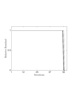
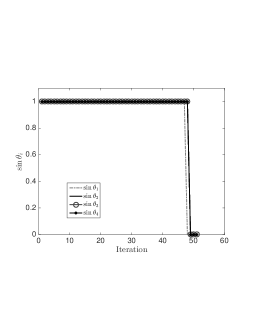
\begin{picture}(0.0,0.0)\end{picture}

Figure 1: Left: Relative two-norm residual curves for stagnating block GMRES and block FOM for the $200\times 200$ shift matrix for four right-hand sides , namely $\mathbf{e}_{1}$, $\mathbf{e}_{50}$, $\mathbf{e}_{100}$, and $\mathbf{e}_{150}$. The solid and dashed curves correspond respectively to the block FOM and GMRES residuals, with each shade of gray representing a different right-hand side. Similarly, the gray solid and dashed curves, respectively, correspond to the second right-hand side. Right: Sines of principal angles between ${\mathcal{R}}\left(\mathbf{F}_{j-1}^{(G)}\right)$ and $A{\mathcal{K}}_{j}(\mathbf{A},\mathbf{F}_{0})$ for each $j$ .

Using the shift matrix $\mathbf{A}_{st}$ with $n=200$, we can construct a problem with four right-hand sides which will stagnate for $50$ iterations before converging exactly. Let the four right-hand sides be the canonical basis vectors $\mathbf{e}_{1}^{[200]}$, $\mathbf{e}_{50}^{[200]}$, $\mathbf{e}_{100}^{[200]}$, and $\mathbf{e}_{150}^{[200]}$. If we let $\mathbf{B}\in\mathbb{R}^{200\times 4}$ be the matrix with these right-hand sides as columns, we know that

$$\mathbf{A}^{-1}_{st}\mathbf{B}=\begin{bmatrix}\mathbf{e}_{200}^{[200]}&\mathbf{e}_{49}^{[200]}&\mathbf{e}_{99}^{[200]}&\mathbf{e}_{149}^{[200]}\end{bmatrix}.$$

Due to the stagnating nature of block GMRES for this problem, we compute the generalized FOM approximation so as to have an iterate at each step. The total stagnation for all four right-hand sides can be seen in Figure 1.

If we arrest the iteration at a stagnating step, e.g., the $40$th step, we can construct the matrices $\widetilde{\mathbf{C}}_{40}$, $\mathbf{C}_{40}$, $\widehat{\mathbf{C}}_{40}$, $\mathbf{N}_{40}$, and $\widehat{\mathbf{N}}_{40}$ (all of which are $4\times 4$ matrices) to see how such matrices, used to verify theoretical results, actually look for a small problem. For the first three matrices, we have the following,

$$\widehat{\mathbf{C}}_{40}=\widetilde{\mathbf{C}}_{40}=\begin{bmatrix}1&&&\\ &-1&&\\ &&-1&\\ &&&-1\end{bmatrix}\mbox{\ \ \ and\ \ \ }\mathbf{C}_{40}=\mathbf{0}_{4},$$

and for the last two matrices we have,

$$\mathbf{N}_{40}=-\mathbf{I}_{4}\mbox{\ \ \ and\ \ \ }\widehat{\mathbf{N}}_{40}=\mathbf{0}_{4}.$$

It should be noted that this agrees with what we have proven about block GMRES in the case of total stagnation in Theorem 3.16 and trivially with Theorem 3.22.

4.2 Partial stagnation/convergence of Block GMRES

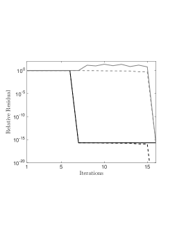
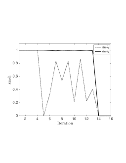
\begin{picture}(0.0,0.0)\end{picture}

Figure 2: Left: Relative two-norm residual curves for stagnating block GMRES and block FOM for the $30\times 30$ shift matrix. The black solid and dashed curves correspond respectively to the block FOM and GMRES residuals for the first right-hand side. Similarly, the gray solid and dashed curves, respectively, correspond to the second right-hand side. Right: Sines of principal angles between ${\mathcal{R}}\left(\mathbf{F}_{j-1}^{(G)}\right)$ and $A{\mathcal{K}}_{j}(\mathbf{A},\mathbf{F}_{0})$ for each $j$ .

In Figure 2, we demonstrate the behavior of block GMRES and Block FOM applied to a linear system for which block GMRES is guaranteed to stagnate but also have earlier convergence for one right-hand side. Here, the coefficient matrix is $\mathbf{A}_{st}$ defined in (46) for $n=30$. The block right-hand side $\mathbf{B}=\begin{bmatrix}\mathbf{e}_{1}^{[30]}&\mathbf{e}_{25}^{[30]}\end{bmatrix}$. From the definition of $\mathbf{A}_{st}$, we have that $\mathbf{A}_{st}^{-1}\mathbf{B}=\begin{bmatrix}\mathbf{e}_{30}^{[30]}&\mathbf{e}_{24}^{[30]}\end{bmatrix}$. From this we see that at iteration $5$, we will achieve exact convergence for the first right-hand side. In the absence of replacing the dependent Arnoldi vector with a random one, the iteration will not produce any improvement for the second right-hand side until iteration $23$, at which point we again have convergence to the exact solution. However, in accordance with our block Arnoldi breakdown strategy, we do replace the the dependent basis vector, meaning we cannot exactly predict stagnation after iteration $5$, though we do see near-stagnation until convergence at iteration $15$.

Again, at a particular iterations, we can inspect various quantities arising which were used in our analysis. We choose three iterations, $j=5,6,11$, to see what happens at breakdown and dependent vector replacement. Indeed we have,

$$\widetilde{\mathbf{C}}_{5} = \begin{bmatrix}1&0\\ 0&-1\end{bmatrix},\mathbf{C}_{5}=\begin{bmatrix}0&0\\ 0&0\end{bmatrix},\mbox{\ \ \ and\ \ \ }\widehat{\mathbf{C}}_{5}=\begin{bmatrix}1&0\\ 0&-1\end{bmatrix}$$

$$\widetilde{\mathbf{C}}_{6} = \begin{bmatrix}0&0\\ -1&0\end{bmatrix},\mathbf{C}_{6}=\begin{bmatrix}0&0\\ -1&0\end{bmatrix},\mbox{\ \ \ and\ \ \ }\widehat{\mathbf{C}}_{6}=\begin{bmatrix}1&0\\ 0&-1\end{bmatrix}$$

$$\widetilde{\mathbf{C}}_{11} \approx \begin{bmatrix}0.97&0\\ -0.22&0\end{bmatrix},\mathbf{C}_{11}\approx\begin{bmatrix}4.16\times 10^{-17}&0\\ -2.22\times 10^{-16}&0\end{bmatrix},\mbox{\ \ \ and\ \ \ }\widehat{\mathbf{C}}_{11}=\begin{bmatrix}0&0\\ -1&0\end{bmatrix}$$

and we also have

$$\mathbf{N}_{5} \approx \begin{bmatrix}-1.00&0\\ 0&-1\end{bmatrix}\mbox{\ \ \ and\ \ \ }\widehat{\mathbf{N}}_{5}\approx\begin{bmatrix}0&0\\ 0&0\end{bmatrix}$$

$$\mathbf{N}_{6} \approx \begin{bmatrix}-1.00&0\\ 0&-1\end{bmatrix}\mbox{\ \ \ and\ \ \ }\widehat{\mathbf{N}}_{6}\approx\begin{bmatrix}0&1\\ 0&0\end{bmatrix}$$

$$\mathbf{N}_{11} \approx \begin{bmatrix}-1.00&-0.02\\ 0&-0.96\end{bmatrix}\mbox{\ \ \ and\ \ \ }\widehat{\mathbf{N}}_{11}\approx\begin{bmatrix}-0.30&0.79\\ 0&-1.11\times 10^{-16}\end{bmatrix}$$

4.3 A less pathological example with sine computation

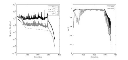
\begin{picture}(0.0,0.0)\end{picture}

Figure 3: In the left-hand figure, we have the $2$-norm residual curves of block GMRES and FOM for a linear system with two right-hand sides using a block diagonal matrix with the sherman4 matrix from [9] as one block and the shift matrix from the other examples as the other block. Right-hand sides are chosen to produce wanted near-stagnation. In the right-hand figure, we have the squares of the sines $\left\{s_{1}^{2},s_{2}^{2}\right\}$ coming from the orthogonal transformations as discussed in the our analysis.

To stimulate some slightly more interesting near stagnation behavior, we created a block diagonal matrix in which one block is sherman4 matrix from the University of Florida Sparse Matrix library [9] and the other block is the shift matrix $\mathbf{A}_{st}$ used in earlier experiments, this time with $n=200$. The two right-hand sides are chose to produce perfect stagnation in the shift-matrix block but convergence in the sherman4 block. Therefore, in the blocks associated to $\mathbf{A}_{st}$, the subvectors of the right-hand sides were $\mathbf{e}_{50}^{[200]}$ and $\mathbf{e}_{150}^{[200]}$. For the sherman4 matrix, the subvectors of the right-hand sides were the vector packaged with the matrix and a random vector scaled to have norm on the order of $10^{7}$. The exaggerated scaling was done only to produce. significant convergence prior to stagnation. In Figure 3, we show the individual $2$-norm block FOM and block GMRES residual curves as well as the sines from the analysis in Section 3.3.

5 Conclusions

In this paper, we have analyzed the relationship of block GMRES and block FOM and specifically characterized this relation in the case of block GMRES stagnation. These results generalize previous results, particularly those in [5] for single vector GMRES and FOM. We have seen that the relationship can be a bit more complicated for block methods than in the single-vector method case due to interaction between approximations for different right-hand sides and due to block Arnoldi breakdown. We close by noting that one can implement block GMRES so that these sines and cosines are cheaply computable, simply by following the strategy advocated in [17] observing that one could implement a version of block GMRES which also cheaply generates the block FOM approximation.

References

- [1] E. Agullo, L. Giraud, and Y.-F. Jing, Block GMRES method with inexact breakdowns and deflated restarting, SIAM Journal on Matrix Analysis and Applications, 35 (2014), pp. 1625–1651, http://dx.doi.org/10.1137/140961912, http://dx.doi.org/10.1137/140961912.
- [2] J. I. Aliaga, D. L. Boley, R. W. Freund, and V. Hernández, A Lanczos-type method for multiple starting vectors, Mathematics of computation, 69 (2000), pp. 1577–1602.
- [3] J. Baglama, Dealing with linear dependence during the iterations of the restarted block Lanczos methods, Numerical Algorithms, 25 (2000), pp. 23–36, http://dx.doi.org/10.1023/A:1016646115432, http://dx.doi.org/10.1023/A:1016646115432.
- [4] S. Birk and A. Frommer, A deflated conjugate gradient method for multiple right hand sides and multiple shifts, Numer. Algorithms, 67 (2014), pp. 507–529, http://dx.doi.org/10.1007/s11075-013-9805-9, http://dx.doi.org/10.1007/s11075-013-9805-9.
- [5] P. N. Brown, A theoretical comparison of the Arnoldi and GMRES algorithms, SIAM J. Sci. Statist. Comput., 12 (1991), pp. 58–78, http://dx.doi.org/10.1137/0912003, http://dx.doi.org/10.1137/0912003.
- [6] A. T. Chronopoulos and A. B. Kucherov, Block--step Krylov iterative methods, Numerical Linear Algebra with Applications, 17 (2010), pp. 3–15, http://dx.doi.org/10.1002/nla.643, http://dx.doi.org/10.1002/nla.643.
- [7] J. Cullum and A. Greenbaum, Relations between Galerkin and norm-minimizing iterative methods for solving linear systems, SIAM J. Matrix Anal. Appl., 17 (1996), pp. 223–247, http://dx.doi.org/10.1137/S0895479893246765, http://dx.doi.org/10.1137/S0895479893246765.
- [8] J. K. Cullum, Peaks, plateaus, numerical instabilities in a Galerkin minimal residual pair of methods for solving , Applied Numerical Mathematics. An IMACS Journal, 19 (1995), pp. 255–278, http://dx.doi.org/10.1016/0168-9274(95)00086-0, http://dx.doi.org/10.1016/0168-9274(95)00086-0. Special issue on iterative methods for linear equations (Atlanta, GA, 1994).
- [9] T. A. Davis and Y. Hu, The University of Florida sparse matrix collection, ACM Transactions in Mathematical Software, 38 (2011), pp. 1:1–1:25, http://dx.doi.org/10.1145/2049662.2049663, http://doi.acm.org/10.1145/2049662.2049663.
- [10] M. Eiermann and O. G. Ernst, Geometric aspects in the theory of Krylov subspace methods, Acta Numerica, 10 (2001), pp. 251–312.
- [11] H. W. Engl, M. Hanke, and A. Neubauer, Regularization of inverse problems, vol. 375 of Mathematics and its Applications, Kluwer Academic Publishers Group, Dordrecht, 1996, http://dx.doi.org/10.1007/978-94-009-1740-8, http://dx.doi.org/10.1007/978-94-009-1740-8.
- [12] R. W. Freund and M. Malhotra, A block QMR algorithm for non-Hermitian linear systems with multiple right-hand sides, Linear Algebra and its Applications, 254 (1997), pp. 119–157, http://dx.doi.org/10.1016/S0024-3795(96)00529-0, http://dx.doi.org/10.1016/S0024-3795(96)00529-0.
- [13] R. W. Freund and N. M. Nachtigal, QMR: a quasi-minimal residual method for non-Hermitian linear systems, Numerische Mathematik, 60 (1991), pp. 315–339, http://dx.doi.org/10.1007/BF01385726, http://dx.doi.org/10.1007/BF01385726.
- [14] G. H. Golub and C. F. Van Loan, Matrix Computations, Johns Hopkins Studies in the Mathematical Sciences, Johns Hopkins University Press, Baltimore, MD, fourth ed., 2013.
- [15] M. H. Gutknecht, Block Krylov space methods for linear systems with multiple right-hand sides: an introduction, in Modern Mathematical Models, Methods and Algorithms for Real World Systems, A. H. Siddiqi, I. S. Duff, and O. Christensen, eds., New Delhi, 2007, Anamaya Publishers, pp. 420–447.
- [16] M. H. Gutknecht and M. Rozložník, By how much can residual minimization accelerate the convergence of orthogonal residual methods?, Numerical Algorithms, 27 (2001), pp. 189–213, http://dx.doi.org/10.1023/A:1011889705659, http://dx.doi.org/10.1023/A:1011889705659.
- [17] M. H. Gutknecht and T. Schmelzer, A QR–decomposition of block tridiagonal matrices generated by the block Lanczos process, in Proceedings of the 17th IMACS World Congress, Paris, 2005, Ecole Central de Lille, Villeneuve d’Ascq, France, July 2005, pp. 1–8. on CD only.
- [18] M. H. Gutknecht and T. Schmelzer, The block grade of a block Krylov space, Linear Algebra and its Applications, 430 (2009), pp. 174–185, http://dx.doi.org/10.1016/j.laa.2008.07.008, http://dx.doi.org/10.1016/j.laa.2008.07.008.
- [19] R. A. Horn and C. R. Johnson, Matrix Analysis, Cambridge University Press, Cambridge, 1985.
- [20] Y.-F. Jing, L. Giraud, B. Carpentieri, and T.-Z. Huang, Recycling block flexible GMRES method with inexact breakdowns for sequences of multiple right-hand side linear systems, In Preparation, (2016).
- [21] J. Langou, Iterative methods for solving linear systems with multiple right-hand sides, PhD thesis, INSA, Toulouse, 2003.
- [22] D. Loher, Reliable nonsymmetric block Lanczos algorithms, PhD thesis, Diss. no. 16337, ETH Zurich, Zurich, Switzerland, 2006.
- [23] A. A. Nikishin and A. Y. Yeremin, Variable block CG algorithms for solving large sparse symmetric positive definite linear systems on parallel computers, I: general iterative scheme, SIAM Journal on Matrix Analysis and Applications, 16 (1995), p. 1135.
- [24] D. P. O’Leary, The block conjugate gradient algorithm and related methods, Linear Algebra and its Applications, 29 (1980), pp. 293–322.
- [25] C. C. Paige and M. Wei, History and generality of the decomposition, Linear Algebra Appl., 208/209 (1994), pp. 303–326, http://dx.doi.org/10.1016/0024-3795(94)90446-4, http://dx.doi.org/10.1016/0024-3795(94)90446-4.
- [26] M. L. Parks, K. Soodhalter, and D. B. Szyld, A block recycled GMRES method with investigations into aspects of solver performance, Tech. Report 16-04-04, Department of Mathematics, Temple University, Apr. 2016.
- [27] M. Robbé and M. Sadkane, A convergence analysis of GMRES and FOM methods for Sylvester equations, Numerical Algorithms, 30 (2002), pp. 71–89, http://dx.doi.org/10.1023/A:1015615310584, http://dx.doi.org/10.1023/A:1015615310584.
- [28] M. Robbé and M. Sadkane, Exact and inexact breakdowns in the block GMRES method, Linear Algebra and its Applications, 419 (2006), pp. 265–285, http://dx.doi.org/10.1016/j.laa.2006.04.018, http://dx.doi.org/10.1016/j.laa.2006.04.018.
- [29] Y. Saad, Variations on Arnoldi’s method for computing eigenelements of large unsymmetric matrices, Linear algebra and its applications, 34 (1980), pp. 269–295.
- [30] Y. Saad, Iterative Methods for Sparse Linear Systems, SIAM, Philadelphia, Second ed., 2003.
- [31] Y. Saad and M. H. Schultz, GMRES: A generalized minimal residual algorithm for solving nonsymmetric linear systems, SIAM Journal on Scientific and Statistical Computing, 7 (1986), pp. 856–869.
- [32] T. Schmelzer, Block Krylov methods for Hermitian linear systems, master’s thesis, 2004.
- [33] V. Simoncini and E. Gallopoulos, An iterative method for nonsymmetric systems with multiple right-hand sides, SIAM Journal on Scientific Computing, 16 (1995), pp. 917–933.
- [34] V. Simoncini and E. Gallopoulos, Convergence properties of block GMRES and matrix polynomials, Linear Algebra and its Applications, 247 (1996), pp. 97–119, http://dx.doi.org/10.1016/0024-3795(95)00093-3, http://dx.doi.org/10.1016/0024-3795(95)00093-3.
- [35] V. Simoncini and D. B. Szyld, Recent computational developments in Krylov subspace methods for linear systems, Numerical Linear Algebra with Applications, 14 (2007), pp. 1–59, http://dx.doi.org/10.1002/nla.499, http://dx.doi.org.libproxy.temple.edu/10.1002/nla.499.
- [36] K. M. Soodhalter, A block MINRES algorithm based on the banded Lanczos method, Numerical Algorithms, 69 (2015), pp. 473–494, http://dx.doi.org/10.1007/s11075-014-9907-z, http://arxiv.org/abs/1301.2102.
- [37] A. Stathopoulos and K. Orginos, Computing and deflating eigenvalues while solving multiple right-hand side linear systems with an application to quantum chromodynamics, SIAM Journal on Scientific Computing, 32 (2010), pp. 439–462, http://dx.doi.org/10.1137/080725532, http://dx.doi.org/10.1137/080725532.
- [38] H. F. Walker, Residual smoothing and peak/plateau behavior in Krylov subspace methods, Appl. Numer. Math., 19 (1995), pp. 279–286, http://dx.doi.org/10.1016/0168-9274(95)00087-9, http://dx.doi.org/10.1016/0168-9274(95)00087-9. Special issue on iterative methods for linear equations (Atlanta, GA, 1994).
- [39] L. Zhou and H. F. Walker, Residual smoothing techniques for iterative methods, SIAM J. Sci. Comput., 15 (1994), pp. 297–312, http://dx.doi.org/10.1137/0915021, http://dx.doi.org/10.1137/0915021.