Internal control for a non-local Schrödinger equation involving the fractional Laplace operator

Abstract.

We analyze the interior controllability problem for a non-local Schrödinger equation involving the fractional Laplace operator $(-\Delta)^{\,s}$, $s\in(0,1)$, on a bounded $C^{1,1}$ domain $\Omega\subset\mathbb{R}^{N}$. We first consider the problem in one space dimension and we employ spectral techniques to prove that, for $s\in[1/2,1)$, null-controllability is achieved by employing an $L^{2}(\omega\times(0,T))$ function acting in a subset $\omega\subset\Omega$ of the domain. This result is then extended to the multi-dimensional case by applying the classical multiplier method, joint with a Pohozaev-type identity for the fractional Laplacian.

1. Introduction and main results

Let $T>0$ be a real number, $\Omega\subset\mathbb{R}^{N}$ be a bounded $C^{1,1}$ domain, $\Omega^{c}:=\mathbb{R}^{N}\setminus\Omega$, and set $Q:=\Omega\times(0,T)$ and $Q^{c}:=\Omega^{c}\times(0,T)$. In this work, we analyze the controllability properties of the following non-local Schrödinger equation

$$\begin{cases}iu_{t}+(-\Delta)^{\,s}u=h\chi_{\omega},&(x,t)\in Q\\ u\equiv 0,&(x,t)\in Q^{c}\\ u(x,0)=u_{0}(x),&x\in\Omega.\end{cases}$$ (1.1)

In (1.1), $u_{0}\in L^{2}(\Omega)$ is a given initial datum and the control $h\in L^{2}(\omega\times(0,T))$ is applied on a neighborhood $\omega$ of the boundary of $\Omega$, defined as

$$\omega:=\mathcal{O}_{\varepsilon}\cap\Omega,\quad\mathcal{O}_{\varepsilon}:=\bigcup_{x\in\Gamma_{0}}B(x,\varepsilon),\quad\varepsilon>0,$$ (1.2)

where

$$\Gamma_{0}=\big{\{}x\in\partial\Omega\,|\,(x\cdot\nu)>0\,\big{\}},\quad\Gamma_{1}=\partial\Omega\setminus\Gamma_{0},$$ (1.3)

and $\nu$ is the unit normal vector to $\partial\Omega$ at $x$ pointing towards the exterior of $\Omega$ (see Figure 1).

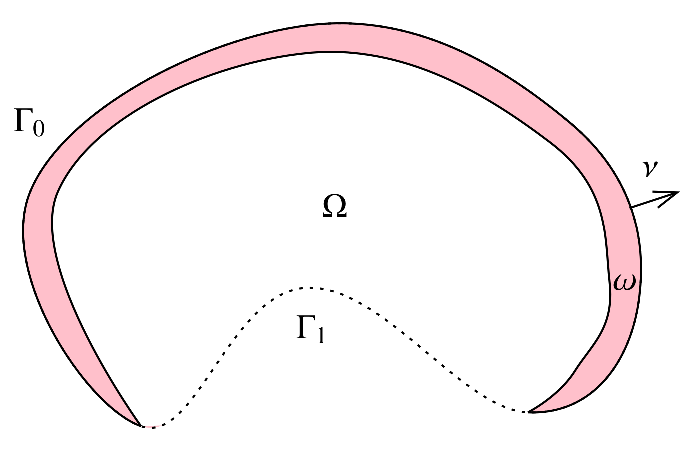
Figure 1. The domain $\Omega$ with the partition $(\Gamma_{0},\Gamma_{1})$ of its boundary and the neighborhood $\omega$ of $\Gamma_{0}$.

Moreover, with $(-\Delta)^{\,s}$ we denote the fractional Laplace operator whose precise definition will be given in the next section.

Fractional order operators (in particular the fractional Laplacian) have recently emerged as a modeling alternative in various branches of science. From the long list of phenomena which are more appropriately modeled by fractional differential equations, we mention: anomalous transport and diffusion ([10, 37]), elasticity ([17]), image processing ([2, 21]), porous media flow ([52]), and population dynamics ([53]). In particular, space-fractional Schrödinger equations have been introduced by Laskin in quantum mechanics [28, 29, 30]), since they provide a natural extension of the standard local model when the Brownian trajectories in Feynman path integrals are replaced by Lévy flights. Applications of this model may be found in the study of a condensed-matter realization of Lévy crystals ([49]). More recently, the fractional Schrödinger equation was introduced into optics by Longhi in [34], with applications to laser implementation. In addition to that, concentration phenomena for the fractional Schrödinger equation have been studied in [14, 15].

Moreover, a number of stochastic models for explaining anomalous diffusion have been introduced in the literature. Among them, we quote the fractional Brownian motion, the continuous time random walk, the Lévy flights, the Schneider grey Brownian motion, and, more generally, random walk models based on evolution equations of single and distributed fractional order in space (see e.g. [18, 22, 36]). In general, a fractional diffusion operator corresponds to a diverging jump length variance in the random walk. In the literature, the fractional Laplace operator is known as the generator of the so called s-stable Lévy process. We refer to [20, 51] and the references therein for further details.

The controllability properties of fractional PDE are still not fully understood by the mathematical community, and only few results are currently available in the literature.

In [5], the null controllability of the one-dimensional fractional heat equation has been treated by using the gap condition on the eigenvalues. This result has been extended to the case of controls acting from the exterior of the domain in [56]. Moreover, the controllability properties of the one-dimensional fractional heat equation under positivity constraints on the control have been studied in [1, 9]. In space dimension $N\geq 2$, the best possible controllability result available for the fractional heat equation is the approximate controllability recently obtained in [55].

Concerning wave-like models, the approximate controllability from the exterior of fractional wave equations has been proved in [35, 57], while [6] treats the null-controllability of a one-dimensional fractional wave equation with memory. Nonetheless, as far as the author knows, there are currently no controllability results for the fractional Schrödinger equation.

In the present paper, we are interested in studying precisely this issue. In more detail, we are going to prove the following result.

Theorem 1.1.

Let $\Omega\subset\mathbb{R}^{N}$ be a bounded $C^{1,1}$ domain and $s\in[1/2,1)$. Moreover, let $\omega\subset\Omega$ be a neighborhood of $\Gamma_{0}$, defined as in (1.2).

1. If $s\in(1/2,1)$, for any $T>0$ and any given initial datum $u_{0}\in L^{2}(\Omega)$ there exists a function $h\in L^{2}(\omega\times(0,T))$ such that the corresponding solution $u$ of (1.1) satisfies $u(x,T)=0$.

2. If $s=1/2$, there exists a strictly positive time $T_{0}>0$ such that the same controllability result as in (i) holds for any $T\geq T_{0}$.

Besides, in both cases there exists a positive constant $\mathcal{C}>0$ such that

$${\left\|h\right\|}_{L^{2}(\omega\times(0,T))}\leq\mathcal{C}\,{\left\|u_{0}\right\|}_{L^{2}(\Omega)}.$$

As it will be clear in the further sections, the requirement of strict positivity of the controllability time when $s=1/2$ arises naturally in the proof of our Theorem (1.1). More details will be given later. We anticipate that, as we will see in Section 3, in the one-dimensional case we can provide an explicit lower estimate for $T_{0}$.

The proof of Theorem 1.1 is based on the classical Hilbert Uniqueness Method (HUM, [13, 31, 32]), according to which the controllability of (1.1) is equivalent to the following observability inequality

$${\left\|v_{0}\right\|}_{L^{2}(\Omega)}^{2}\leq\mathcal{C}\int_{0}^{T}{\left\|v(t)\right\|}_{L^{2}(\omega)}^{2}\,dt,$$ (1.4)

where, for any $v_{0}\in L^{2}(\Omega)$, $v$ is the solution of the adjoint system

$$\begin{cases}iv_{t}+(-\Delta)^{\,s}v=0,&(x,t)\in Q\\ v\equiv 0,&(x,t)\in Q^{c}\\ v(x,0)=v_{0}(x),&x\in\Omega.\end{cases}$$ (1.5)

For obtaining this inequality, we will distinguish two cases in which we will use different methodologies:

• In one space dimension, (1.4) will be proved by employing spectral techniques and Ingham-type estimates ([24]), following the by now standard approach described, for instance, in [38]. In this framework, we will also show that $s\in[1/2,1)$ is a necessary condition for the positivity of the controllability result. Indeed, our analysis yields that, at least in one space-dimension, when the power of the fractional Laplacian is below the critical value $s=1/2$, equation (1.1) fails to be controllable. This fact is a direct consequence of the spectral results contained in [26, 27]. For completeness, we shall stress that, as we will see in Section 3, for the employment of the mentioned spectral techniques the requirement that $\omega$ is a neighborhood of the boundary is actually not necessary. Therefore, in the one-dimensional case the support of the control may be any general open subset.

• In dimension $N\geq 2$, (1.4) will be obtained by applying the multiplier method ([25]) and a Pohozaev-type identity for the fractional Laplacian, which has been proved in [44] and extends to the fractional case the well-known identity due to Pohozaev (see [39]).

The rest of the paper is organized as follows. Section 2 is devoted to the presentation of the functional setting in which we will work. Moreover, we recall there some results related to the fractional Laplace operator, the regularity of the associated Dirichlet problem, the Pohozaev-type identity and the principal spectral properties in the one-dimensional case. We conclude the section by discussing the well-posedness of the fractional Schrödinger equation (1.1). In Section 3, we treat the one-dimensional controllability problem by employing standard spectral techniques. Section 4 will be devoted to the multi-dimensional case. We start by obtaining a Pohozaev-type identity for (1.1), which we will later apply for proving the observability inequality (1.4). Our main result, Theorem 1.1, will then be a consequence of this inequality. Finally, Section 5 is devoted to some open problems and perspectives related to our work.

2. Fractional Laplace operator: definition, Dirichlet problem and Pohozaev-type identity

In this Section, we introduce some preliminary results that will be useful in the remainder of the paper.

We start by giving a rigorous definition of the fractional Laplace operator. To this end, for $s\in(0,1)$, let us consider the space

$$\mathcal{L}^{1}_{s}\left(\mathbb{R}^{N}\right):=\left\{u:\mathbb{R}^{N}\longrightarrow\mathbb{R}^{N}\,:\;u\textrm{ measurable },\;\int_{\mathbb{R}^{N}}\frac{|u(x)|}{(1+|x|)^{N+2s}}\,dx<+\infty\right\}.$$

For any $u\in\mathcal{L}_{s}^{1}\left(\mathbb{R}^{N}\right)$ and $\varepsilon>0$, we set

$$(-\Delta)^{s}_{\varepsilon}\,u(x)=c_{N,s}\,\int_{|x-y|>\varepsilon}\frac{u(x)-u(y)}{|x-y|^{N+2s}}\,dy,\;\;\;x\in\mathbb{R}^{N},$$

with $c_{N,s}$ an explicit normalization constant given by

$$c_{N,s}:=\frac{s2^{2s}\Gamma\left(\frac{N+2s}{2}\right)}{\pi^{N/2}\Gamma(1-s)},$$

$\Gamma$ being the Euler Gamma function. The fractional Laplacian is then defined by the following singular integral

$$(-\Delta)^{\,s}u(x)=c_{N,s}\,P.V.\,\int_{\mathbb{R}^{N}}\frac{u(x)-u(y)}{|x-y|^{N+2s}}\,dy=\lim_{\varepsilon\to 0^{+}}(-\Delta)^{s}_{\varepsilon}u(x),\;\;\;x\in\mathbb{R}^{N},$$ (2.1)

provided that the limit exists.

We notice that, if $s\in(0,1/2)$ and $u$ is a smooth function, for example bounded and Lipschitz continuous on $\mathbb{R}^{N}$, then the integral in (2.1) is in fact not really singular near $x$ (see e.g. [16, Remark 3.1]). Moreover, $\mathcal{L}_{s}^{1}\left(\mathbb{R}^{N}\right)$ is the right space for which $v:=(-\Delta)^{s}_{\varepsilon}\,u$ exists for every $\varepsilon>0$, $v$ being also continuous at the continuity points of $u$ (see [54]).

We also mention that the fractional Laplace operator is a pseudo-differential operator with symbol $|\xi|^{2s}$ (see, e.g., [16, Proposition 3.3]). For more details on the fractional Laplacian we refer to [16, 51, 54] and the references therein.

Let us now define the function spaces in which we are going to work. It is well-known (see, e.g., [16]) that the natural functional setting for problems involving the fractional Laplacian is the one of the fractional Sobolev spaces. Since these spaces are not as familiar as the classical integral order ones, for the sake of completeness, we recall here their definition and some fundamental properties.

Given $s\in(0,1)$ and $\Omega\subset\mathbb{R}^{N}$ a regular enough domain, the fractional Sobolev space $H^{s}(\Omega)$ is defined as

$$H^{s}(\Omega):=\left\{u\in L^{2}(\Omega)\,:\,\frac{|u(x)-u(y)|}{|x-y|^{\frac{N}{2}+s}}\in L^{2}(\Omega\times\Omega)\right\}.$$

It is classical that this is a Hilbert space, endowed with the norm (derived from the scalar product)

$${\left\|u\right\|}_{H^{s}(\Omega)}:=\Big{(}{\left\|u\right\|}_{L^{2}(\Omega)}^{2}+|u|_{H^{s}(\Omega)}^{2}\,\Big{)}^{\frac{1}{2}},$$

where the term

$$|u|_{H^{s}(\Omega)}:=\left(\int_{\Omega}\int_{\Omega}\frac{|u(x)-u(y)|^{2}}{|x-y|^{N+2s}}\,dxdy\right)^{\frac{1}{2}}$$

is the so-called Gagliardo semi-norm of $u$. Let us now denote

$$H^{s}_{0}(\Omega):=\overline{C^{\infty}_{0}(\Omega)}^{\,H^{s}(\Omega)}$$

the closure of the continuous infinitely differentiable functions with compact support in $\Omega$ with respect to the $H^{s}(\Omega)$-norm. The following facts are well-known.

• For $0<s\leq 1/2$, the identity $H^{s}_{0}(\Omega)=H^{s}(\Omega)$ holds. This is because, in this case, the $C^{\infty}_{0}(\Omega)$ functions are dense in $H^{s}(\Omega)$ (see, e.g., [33, Theorem 11.1]).

• For $1/2<s<1$, we have $H^{s}_{0}(\Omega)=\left\{u\in H^{s}(\mathbb{R}^{N})\,:\,u=0\textrm{ in }\Omega^{c}\right\}$ (see [19]).

Finally, in what follows, we will indicate with $H^{-s}(\Omega)=\left(H^{s}(\Omega)\right)^{\ast}$ the dual of $H^{s}(\Omega)$ with respect to the pivot space $L^{2}(\Omega)$.

We now present a couple of results which will be used in the rest of the paper. Let us consider the Dirichlet problem associated to the fractional Laplace operator

$$\left\{\begin{array}[]{rl}(-\Delta)^{\,s}u=g,&x\in\Omega,\\ u\equiv 0,&x\in\Omega^{c}.\end{array}\right.$$ (2.4)

By means of the Lax-Milgram Lemma (see, e.g., [8, Proposition 2.1]), it is not difficult to see that, if $g\in H^{-s}(\Omega)$, then (2.4) admits a unique solution $u\in H_{0}^{s}(\Omega)$ satisfying the norm estimate

$${\left\|u\right\|}_{H^{s}(\Omega)}\leq\mathcal{C}{\left\|g\right\|}_{H^{-s}(\Omega)},$$ (2.5)

where $\mathcal{C}$ is a positive constant independent of $g$. Moreover, in [8, Theorem 1.3], the following local regularity property for (2.4) has been obtained.

Proposition 2.1.

Let $g\in H^{-s}(\Omega)$ and let $u\in H^{s}_{0}(\Omega)$ be the unique weak solution to the Dirichlet problem (2.4). If $g\in L^{2}(\Omega)$, then $u\in H^{2s}_{loc}(\Omega)$.

Notice that, when $s\geq 1/2$, Proposition 2.1 and classical embedding results for the fractional Sobolev spaces (see, e.g., [16, Proposition 2.1]) yield that the solution of (2.4) is in $H^{1}_{loc}(\Omega)$.

In addition to that, in [44, Proposition 1.6] the following has been proved.

Proposition 2.2.

Let $\Omega$ be a bounded $C^{1,1}$ domain of $\mathbb{R}^{N}$, $s\in(0,1)$ and $\delta(x)=\mbox{dist}(x,\partial\Omega)$, with $x\in\Omega$, be the distance of a point $x$ from $\partial\Omega$. Let $u\in H_{0}^{s}(\Omega)$ satisfy the following:

• $u\in C^{s}(\mathbb{R}^{N})$ and, for every $\beta\in[s,1+2s)$, $u$ is of class $C^{\beta}(\Omega)$ and

  $$[u]_{C^{\beta}(\{x\in\Omega|\delta(x)\geq\rho\})}\leq\mathcal{C}\rho^{s-\beta},\;\;\;\textrm{ for all }\rho\in(0,1).$$

• The function $u/\delta^{s}|_{\Omega}$ can be continuously extended to $\overline{\Omega}$. Moreover, there exists $\gamma\in(0,1)$ such that $u/\delta^{s}\in C^{\gamma}(\overline{\Omega})$. In addition, for all $\beta\in[\gamma,s+\gamma]$ it holds the estimate

  $$[u/\delta^{s}]_{C^{\beta}(\{x\in\Omega|\delta(x)\geq\rho\})}\leq\mathcal{C}\rho^{\gamma-\beta},\;\;\;\textrm{ for all }\rho\in(0,1).$$

• $(-\Delta)^{\,s}u$ is point-wise bounded in $\Omega$.

Then, the following identity holds

$$\int_{\Omega}(x\cdot\nabla u)(-\Delta)^{\,s}u\,dx=\frac{2s-N}{2}\int_{\Omega}u(-\Delta)^{\,s}u\,dx-\frac{\Gamma(1+s)^{2}}{2}\int_{\partial\Omega}\left(\frac{u}{\delta^{s}}\right)^{2}(x\cdot\nu)\,d\sigma,$$ (2.6)

where $\nu$ is the unit outward normal to $\partial\Omega$ at $x$ and $\Gamma$ is the Gamma function.

In the Proposition 2.2, following the notation introduced in [42, 43, 44], $C^{\beta}(\Omega)$ with $\beta>0$ indicates the space $C^{k,\,\beta^{\prime}}(\Omega)$, where $k$ is the greatest integer such that $k<\beta$ and $\beta^{\prime}=\beta-k$.

Finally, in the remaining of our work we will also need the following technical results.

Proposition 2.3.

Let $u$,$v$ be two functions in $H^{s}_{0}(\Omega)$. Then, it holds the integration formula

$$\int_{\Omega}v(-\Delta)^{\,s}udx=\int_{\mathbb{R}^{N}}(-\Delta)^{\,\frac{s}{2}}u(-\Delta)^{\,\frac{s}{2}}vdx=\int_{\Omega}u(-\Delta)^{\,s}vdx.$$ (2.7)

Proof.

The proof of (2.7) is a simple application of Plancherel’s theorem and the fact that the fractional Laplacian is the pseudo-differential operator associated to the symbol $|\xi|^{2s}$, that is

$$(-\Delta)^{\,s}u=\mathscr{F}^{-1}\bigg{(}|\xi|^{2s}\mathscr{F}u\bigg{)},\;\;\textrm{ for all }\xi\in\mathbb{R}^{N},\;u\in H^{s}(\mathbb{R}^{N}).$$

To avoid any issue on the domain of $\mathscr{F}$ and $\mathscr{F}^{-1}$ one shall first take $u\in C_{0}^{\infty}(\Omega)$ and then use density properties. We leave the details to the reader. ∎

Proposition 2.4.

Let $\Omega\subset\mathbb{R}^{N}$ be a bounded regular domain. For every $g,h\in H^{1}_{0}(\Omega)$, let us define

$$T(g,h):=\int_{\Omega}\overline{g}(x\cdot\nabla h)\,dx.$$

Then, for all $s\in[1/2,1)$ there exists a positive constant $\mathcal{C}$, depending only on $N$, $s$ and $\Omega$, such that

$$|T(g,h)|\leq\mathcal{C}\,{\left\|g\right\|}_{H^{1-s}_{0}(\Omega)}{\left\|h\right\|}_{H^{s}_{0}(\Omega)}$$ (2.8)

and

$$|T(g,h)|\leq\mathcal{C}\,{\left\|g\right\|}_{H^{s}_{0}(\Omega)}{\left\|h\right\|}_{H^{s}_{0}(\Omega)}.$$ (2.9)

Proof.

The result follows by a simple interpolation argument. First of all, since $\Omega$ is bounded, we have

$$\left|\int_{\Omega}\overline{g}(x\cdot\nabla h)\,dx\,\right|\leq\mathcal{C}_{1}(\Omega){\left\|g\right\|}_{L^{2}(\Omega)}{\left\|h\right\|}_{H_{0}^{1}(\Omega)}$$ (2.10)

Moreover, integrating by parts and using Poincaré’s inequality we get

$$\left|\int_{\Omega}\overline{g}(x\cdot\nabla h)\,dx\,\right| =\left|\int_{\Omega}\left(\nabla\overline{g}\cdot xh+N\overline{g}h\right)\,dx\,\right|$$

$$\leq\mathcal{C}(\Omega){\left\|g\right\|}_{H_{0}^{1}(\Omega)}{\left\|h\right\|}_{L^{2}(\Omega)}+N{\left\|g\right\|}_{L^{2}(\Omega)}{\left\|h\right\|}_{L^{2}(\Omega)}\leq\mathcal{C}_{2}(N,\Omega){\left\|g\right\|}_{H_{0}^{1}(\Omega)}{\left\|h\right\|}_{L^{2}(\Omega)}.$$ (2.11)

From (2.10) and (2) we have that $T\in\mathcal{L}(H_{0}^{1}(\Omega)\times L^{2}(\Omega))\cap\mathcal{L}(L^{2}(\Omega)\times H_{0}^{1}(\Omega))$. Therefore, applying [33, Chapter 1, Theorems 5.1, 12.2 and 12.3] we have $T\in\mathcal{L}(H^{1-s}_{0}(\Omega)\times H^{s}_{0}(\Omega))$ and, consequently,

$$|T(g,h)|\leq\mathcal{C}\,{\left\|g\right\|}_{H^{1-s}_{0}(\Omega)}{\left\|h\right\|}_{H^{s}_{0}(\Omega)},$$

with $\mathcal{C}=\mathcal{C}(N,s,\Omega)$. Finally, the second inequality

$$|T(g,h)|\leq\mathcal{C}\,{\left\|g\right\|}_{H^{s}_{0}(\Omega)}{\left\|h\right\|}_{H^{s}_{0}(\Omega)},$$

is trivial since, for $s\geq 1/2$, by [16, Proposition 2.1], we have $H^{s}_{0}(\Omega)\hookrightarrow H^{1-s}_{0}(\Omega)$ with continuous injection. ∎

2.1. The one-dimensional fractional Laplacian

In this Section, we focus on the one-dimensional case and we present the main spectral properties of the fractional Laplacian. For the rest of this sub-section, let $\Omega=(-1,1)$ and denote by $(-d_{x}^{\,2})^{s}_{D}$ the self-adjoint operator on $L^{2}(-1,1)$ associated with the closed and bilinear form

$$\mathcal{E}(u,v)=\frac{c_{1,s}}{2}\int_{\mathbb{R}}\int_{\mathbb{R}}\frac{(u(x)-u(y))(v(x)-v(y))}{|x-y|^{1+2s}}\;dxdy,\;\;u,v\in H_{0}^{s}(-1,1).$$

More precisely,

$$D((-d_{x}^{\,2})^{s}_{D})=\Big{\{}u\in H_{0}^{s}(-1,1):\;(-d_{x}^{\,2})^{s}u\in L^{2}(-1,1)\Big{\}},\quad(-d_{x}^{\,2})^{s}_{D}u=(-d_{x}^{\,2})^{s}u\;\mbox{ in }\;(-1,1).$$

We refer to [12] for a rigorous and precise definition of $(-d_{x}^{\,2})^{s}_{D}$.

Then $(-d_{x}^{\,2})^{s}_{D}$ is the realization in $L^{2}(-1,1)$ of the fractional Laplace operator $(-d_{x}^{\,2})^{s}$ with the zero Dirichlet exterior condition $u=0$ in $(-1,1)^{c}$. It is well-known (see e.g. [46]) that $(-d_{x}^{\,2})^{s}_{D}$ has a compact resolvent and its eigenvalues form a non-decreasing sequence of real numbers

$$0<\lambda_{1}\leq\lambda_{2}\leq\cdots\leq\lambda_{k}\leq\cdots$$

satisfying $\lim_{k\to+\infty}\lambda_{k}=+\infty$. In addition to that, the eigenvalues are of finite multiplicity.

Let $(\phi_{k})_{k\geq 1}$ be the orthonormal basis of eigenfunctions associated with the eigenvalues $(\lambda_{k})_{k\geq 1}$, that is,

$$\begin{cases}(-d_{x}^{\,2})^{s}\phi_{k}=\lambda_{k}\phi_{k},&x\in(-1,1),\quad k\geq 1\\ \phi_{k}=0&x\in(-1,1)^{c},\end{cases}$$ (2.12)

and let $s<1/2$. Then, according to [45, Proposition 9], the eigenvalues $(\lambda_{k})_{k\geq 1}$ can be characterized as

$$\lambda_{k+1}=\min_{\underset{{\left\|\phi\right\|}_{L^{2}(-1,1)}=1}{\phi\in\mathbb{P}_{k+1}}}\int_{\mathbb{R}}\int_{\mathbb{R}}\frac{|\phi(x)-\phi(y)|^{2}}{|x-y|^{1+2s}}\,dxdy=\min_{\underset{{\left\|\phi\right\|}_{L^{2}(-1,1)}=1}{\phi\in\mathbb{P}_{k+1}}}[\phi]_{H^{s}(\mathbb{R})}^{2},\;\;\textrm{ for all }k\geq 1$$ (2.13)

or, equivalently,

$$\lambda_{k+1}=\min_{\phi\in\mathbb{P}_{k+1}\setminus\{0\}}\frac{\displaystyle\int_{\mathbb{R}}\int_{\mathbb{R}}\frac{|\phi(x)-\phi(y)|^{2}}{|x-y|^{1+2s}}\,dxdy}{\displaystyle\int_{-1}^{1}|\phi|^{2}\,dx}=\min_{\phi\in\mathbb{P}_{k+1}\setminus\{0\}}\frac{[\phi]_{H^{s}(\mathbb{R})}^{2}}{{\left\|\phi\right\|}_{L^{2}(-1,1)}^{2}},\;\textrm{ for all }k\geq 1.$$ (2.14)

Here $\mathbb{P}_{k+1}$ denotes the space

$$\mathbb{P}_{k+1}:=\Big{\{}\phi\in L^{2}(-1,1)\,:\,\phi=0\textrm{ a.e. in }(-1,1)^{c},\;\langle\phi,\phi_{j}\rangle_{L^{2}(-1,1)}=0\textrm{ for all }j=1,\ldots,k\Big{\}}.$$

Moreover, the eigenfunction $\phi_{k+1}$ is precisely the element of $\mathbb{P}_{k+1}$ attaining the minimum in (2.13), that is,

$$\lambda_{k+1}=[e_{k+1}]_{H^{s}(\mathbb{R})}^{2},\;\;\textrm{ for all }k\geq 1.$$

To the best of our knowledge, characterizations of the spectrum of the fractional Laplacian analogous to (2.13), (2.14) are not available when $s\geq 1/2$. Nevertheless, we have the following asymptotic result of the eigenvalues, whose proof is contained in [27, Proposition 3], that will be needed in our further analysis.

Lemma 2.5.

Let $1/2\leq s<1$, $\Omega=(-1,1)$ and $(\lambda_{k})_{k\geq 1}$ be the eigenvalues of $(-d_{x}^{2})^{s}_{D}$. Then the following assertions hold.

1. The eigenvalues $(\lambda_{k})_{k\geq 1}$ are simple.

2. There is a constant $\gamma=\gamma(s)\geq\pi/2$ such that for $k$ large enough,

   $$\lambda_{k+1}-\lambda_{k}\geq\gamma.$$ (2.15)

2.2. Well-posedness

Let us conclude this section by proving the existence and uniqueness of solutions for the fractional Schrödinger equation (1.1).

To this end, let us denote by $\mathcal{A}$ the realization of $(-\Delta)^{\,s}$ in $L^{2}(\Omega)$ with zero Dirichlet exterior condition, i.e., the operator $\mathcal{A}:\mathcal{D}(\mathcal{A})\rightarrow L^{2}(\Omega)$ defined as

$$\mathcal{D}(\mathcal{A})=\left\{u\in H_{0}^{s}(\Omega)\,\Big{|}\,(-\Delta)^{\,s}u\in L^{2}(\Omega)\,\right\},\;\;\;\mathcal{A}u:=-(-\Delta)^{\,s}u.$$ (2.16)

See [54] for more details. Moreover, we mention that $\mathcal{D}(\mathcal{A})$ has been fully characterized in [23], by employing standard pseudo-differential techniques.

It is classically known that the operator $\mathcal{A}$ is self-adjoint and negative. Therefore, thanks to the Stone’s theorem ([59, Chapter XI, Section 13, Theorem 1]), $i\mathcal{A}$ is the generator of a one parameter $C_{0}$ group of unitary operators and we have the following well-posedness result (see [11, Lemmas 4.1.1 and 4.1.5]).

Theorem 2.6.

Given $u_{0}\in L^{2}(\Omega)$ and $h\in L^{2}(\omega\times(0,T))$, the system (1.1) admits a unique solution

$$u\in C\big{(}[0,T];L^{2}(\Omega)\big{)}.$$

Moreover, if $u_{0}\in\mathcal{D}(\mathcal{A})$ then

$$u\in C\big{(}[0,T];\mathcal{D}(\mathcal{A})\big{)}\cap C^{1}\big{(}[0,T];L^{2}(\Omega)\big{)}.$$

3. The one dimensional controllability problem

This section is devoted to the analysis of the controllability of (1.1) in the one-dimensional case. In particular, we are going to prove here that, when $N=1$, the fractional Schrödinger equation (1.1) is null controllable by means of an interior control $h$ supported in an open subset $\omega\subset(-1,1)$ if and only if $s\geq 1/2$. Thus, the main result of this section will be the following Theorem.

Theorem 3.1.

Let $\omega\subset(-1,1)$ and $T>0$. Let us consider the following control problem for the one-dimensional fractional Schrödinger equation on the interval $(-1,1)$

$$\left\{\begin{array}[]{ll}iu_{t}+(-d_{x}^{\,2})^{s}u=g\chi_{\omega},&(x,t)\in(-1,1)\times(0,T),\\ u\equiv 0,&(x,t)\in(-1,1)^{c}\times(0,T),\\ u(x,0)=u_{0}(x),&x\in(-1,1).\end{array}\right.$$ (3.4)

1. If $s\in(1/2,1)$, for any $T>0$ and any given $u_{0}\in L^{2}(-1,1)$, there exists $g\in L^{2}(\omega\times(0,T))$ such that the solution $u$ of (3.4) satisfies $u(x,T)=0$.

2. If $s=1/2$, for any $T>4$ and any given $u_{0}\in L^{2}(-1,1)$, there exists $g\in L^{2}(\omega\times(0,T))$ such that the solution $u$ of (3.4) satisfies $u(x,T)=0$.

Proof of Theorem 3.1.

We recall that, by means of HUM, the controllability of (3.4) is equivalent to the observability of the adjoint equation

$$\left\{\begin{array}[]{ll}iv_{t}+(-d_{x}^{\,2})^{s}v=0,&(x,t)\in(-1,1)\times(0,T),\\ v\equiv 0,&(x,t)\in(-1,1)^{c}\times(0,T),\\ v(x,0)=v_{0}(x),&x\in(-1,1).\end{array}\right.$$ (3.8)

In other words, it will be enough to show that, for all solution $v$ to (3.8), it holds the inequality

$${\left\|v_{0}\right\|}_{L^{2}(-1,1)}^{2}\leq\mathcal{C}\int_{0}^{T}{\left\|v(t)\right\|}_{L^{2}(\omega)}\,dt.$$ (3.9)

To this end, let us write the solution of (3.8) in terms of the spectrum of the Dirichlet fractional Laplacian on $(-1,1)$, that is,

$$v(x,t)=\sum_{k\geq 1}v_{k}e^{i\lambda_{k}t}\phi_{k}(x),$$ (3.10)

with

$$v_{k}=\int_{-1}^{1}v_{0}(x)\phi_{k}(x)\,dx.$$

From (3.10), by using the orthonormality of the eigenfunctions in $L^{2}(-1,1)$, it is immediate to see that the observability inequality (3.9) may be rewritten as

$$\sum_{k\geq 1}|v_{k}|^{2}\leq\mathcal{C}\int_{0}^{T}\int_{\omega}\left|\sum_{k\geq 1}v_{k}e^{i\lambda_{k}t}\phi_{k}(x)\,\right|^{2}\,dxdt.$$ (3.11)

In order to obtain (3.11) we will employ classical Ingham’s techniques (see, e.g., [24], [38, Section 4] or [50, Chapter 8, Theorem 8.1.1]). In particular, in [38, Theorem 4.3] it has been proven that, if there is a positive gap between the eigenvalues, namely

$$\liminf_{k\to+\infty}(\lambda_{k+1}-\lambda_{k})=\gamma_{\infty}>0,$$ (3.12)

then, for any finite real time $T>2\pi/\gamma_{\infty}$ and any finite sequence $\{a_{k}\}_{k\geq 1}$, it holds the inequality

$$\sum_{k\geq 1}|a_{k}|^{2}\leq\mathcal{C}(T)\int_{0}^{T}\left|\sum_{k\geq 1}a_{k}e^{i\lambda_{k}t}\,\right|^{2}\,dt,$$ (3.13)

where the constant $\mathcal{C}(T)$ depends only on the time horizon $T$.

Moreover, employing the asymptotic results on the spectrum of the fractional Laplacian contained in the papers [26, 27], we can easily show that, for any sub-interval $\omega\subset(-1,1)$, there exists a positive constant $\beta>0$ such that it holds the lower estimate

$${\left\|\phi_{k}\right\|}_{L^{2}(\omega)}\geq\beta>0.$$ (3.14)

We mention that (3.14) can be also obtained as a direct consequence of [9, Lemma 3.2], where the same inequality in the $L^{1}$ setting has been proved.

Let us now fix $x\in(-1,1)$. Taking $a_{k}=v_{k}\phi_{k}(x)$ in (3.13) we obtain that there is a constant $\mathcal{C}(T)$, independent of $x$, such that it holds the inequality

$$\sum_{k\geq 1}|v_{k}\phi_{k}(x)|^{2}\leq\mathcal{C}(T)\int_{0}^{T}\left|\sum_{k\geq 1}v_{k}e^{i\lambda_{k}t}\phi_{k}(x)\,\right|^{2}\,dt.$$ (3.15)

Then, integrating (3.15) over $\omega$ and using the estimate (3.14), we get that

$$\beta\sum_{k\geq 1}|v_{k}|^{2}\leq\int_{\omega}\sum_{k\geq 1}|v_{k}\phi_{k}(x)|^{2}\,dx\leq\mathcal{C}(T)\int_{\omega}\int_{0}^{T}\left|\sum_{k\geq 1}v_{k}e^{i\lambda_{k}t}\phi_{k}(x)\,\right|^{2}\,dtdx,$$

which is clearly equivalent to (3.11).

Hence, in order to conclude our proof, it only remains to check whether (3.13) holds in our case. In other words, we shall see if the gap condition (3.12) is satisfied.

To this end, we recall that from [27, Theorem 1] (see also Lemma 2.5) we know that the eigenvalues of the Dirichlet fractional Laplacian on $(-1,1)$ are given by

$$\lambda_{k}=\left(\frac{k\pi}{2}-\frac{(2-2s)\pi}{8}\right)^{2s}+O\left(\frac{1}{k}\right),\;\;\;\textrm{ as }k\to+\infty,$$

while [27, Propositon 3] ensures that $\lambda_{k}$ are simple if $s\geq 1/2$ (see Figures 2 and 3). In particular, we can readily check that

$$\gamma_{\infty}=\liminf_{k\to+\infty}(\lambda_{k+1}-\lambda_{k})=\begin{cases}0,&s<1/2\\ \pi/2,&s=1/2\\ +\infty,&s>1/2.\end{cases}$$

Figure 2. First 15 eigenvalues of the Dirichlet fractional Laplacian $(-d_{x}^{\,2})^{s}$ on $(-1,1)$ for $s\in(0,1/2]$ (left) and $s\in(1/2,1)$ (right).

Figure 3. Gap between the first 15 eigenvalues of the Dirichlet fractional Laplacian $(-d_{x}^{\,2})^{s}$ on $(-1,1)$ for $s\in(0,1/2]$ (left) and $s\in(1/2,1)$ (right).

This, in turn, implies that (3.13) (and, consequently, (3.9)) holds for any $T>4/\pi$, if $s=1/2$, and for all $T>0$, if $s>1/2$. Our proof is then concluded. ∎

4. Fractional Schrödinger equation

We address now the multi-dimensional case, in which the observability inequality (1.4) will be obtained by employing the nowadays classical multiplier method. To this end, a series of preliminary technical results will be needed.

4.1. Pohozaev-type identity

In this Section, we introduce one of the main tools that are needed in order to prove the controllability Theorem 1.1: a Pohozaev-type identity for the solution of our fractional Schrödinger equation. This identity will be obtained employing the classical multiplier method (see, e.g., [25, 31, 32]), joint with the Pohozaev identity for the fractional Laplacian that we introduced in Proposition 2.2 (see also [44, Proposition 1.6]).

Proposition 4.1.

Let $\Omega$ be a bounded $C^{1,1}$ domain of $\mathbb{R}^{N}$, $s\in[1/2,1)$ and $\delta(x)$ be the distance of a point $x$ from $\partial\Omega$. Moreover, let $\mathcal{D}(\mathcal{A})$ be defined as in (2.16). For any $h\in L^{2}(\Omega\times(0,T))$ and any initial datum $u_{0}\in\mathcal{D}(\mathcal{A})$, let $u$ be the corresponding solution of (1.1). Then, the following identity holds

$$\Gamma(1+s)^{2}\int_{\Sigma}\left(\frac{|u|}{\delta^{s}}\right)^{2}(x\cdot\nu)\,d\sigma dt= \,2s\int_{0}^{T}\left\|(-\Delta)^{\,\frac{s}{2}}u(t)\right\|^{2}_{L^{2}(\mathbb{R}^{N})}\,dt+\Im\int_{\Omega}\overline{u}(x\cdot\nabla u)\,\big{|}_{0}^{T}\,dx$$

$$-\Re\int_{0}^{T}\int_{\omega}h\,\Big{(}N\overline{u}+2x\cdot\nabla\overline{u}\,\Big{)}\,dxdt,$$ (4.1)

where $\nu$ is the unit outward normal to $\partial\Omega$ at $x$, $\Gamma$ is the Gamma function and $\Sigma:=\partial\Omega\times[0,T]$.

Proof.

For proving Proposition 4.1, we are going to apply the classical method of multipliers (see [25, 31, 32]), joint with the Pohozaev identity for the fractional Laplacian that we introduced in Proposition 2.2 (see also [44, Proposition 1.6]).

However, this mentioned identity holds under very strict regularity assumptions, which are not necessarily satisfied by the solution $u$ of (1.1).

In order to bypass this regularity issue, we can first obtain (4.1) for solutions of (1.1) corresponding to an initial datum $u_{0}$ given as a linear combination of a finite number of eigenfunctions of the Dirichlet fractional Laplacian on $\Omega$. Indeed, it follows from [47, Proposition 4] and [42, Corollary 1.6] that the Pohozaev identity holds in this case.

In a second moment, we can recover the result for any finite energy solution $u$ by using a compactness argument. Since this compactness argument is a standard one, in order to abridge our presentation, in what follows we will skip it and we will always assume that we have all the required regularity to perform our computations.

Let us now prove the identity (4.1). To this end, we multiply our equation (1.1) by $x\cdot\nabla\overline{u}+(N/2)\overline{u},$ we take the real part, and we integrate over $Q$, obtaining

$$\Re\int_{0}^{T}\int_{\omega}h\left(x\cdot\nabla\overline{u}+\frac{N}{2}\overline{u}\right)\,dxdt= \underbrace{\Re\int_{Q}(-\Delta)^{\,s}u(x\cdot\nabla\overline{u})\,dxdt}_{A_{1}}\;+\underbrace{\Re\int_{Q}\frac{N}{2}\overline{u}(-\Delta)^{\,s}u\,dxdt}_{A_{2}}$$

$$+\underbrace{\Re\int_{Q}iu_{t}\left(\frac{N}{2}\overline{u}+x\cdot\nabla\overline{u}\right)\,dxdt.}_{A_{3}}$$

We now compute the three contributions on the right-hand side separately. For the first integral, employing (2.6), we have

$$A_{1}= \int_{Q}\bigg{\{}\Big{[}(-\Delta)^{\,s}\Re(u)\Big{]}\Big{(}x\cdot\nabla\Re(u)\Big{)}+\Big{[}(-\Delta)^{\,s}\Im(u)\Big{]}\Big{(}x\cdot\nabla\Im(u)\Big{)}\bigg{\}}\,dxdt$$

$$= \,\frac{2s-N}{2}\int_{Q}\bigg{\{}\Re(u)\Re\big{[}(-\Delta)^{\,s}u\big{]}+\Im(u)\Im\big{[}(-\Delta)^{\,s}u\big{]}\bigg{\}}\,dxdt$$

$$-\frac{\Gamma(1+s)^{2}}{2}\int_{\Sigma}\left[\left(\frac{\Re(u)}{\delta^{s}}\right)^{2}+\left(\frac{\Im(u)}{\delta^{s}}\right)^{2}\right](x\cdot\nu)\,d\sigma dt$$

$$= \,\frac{2s-N}{2}\,\Re\int_{Q}\overline{u}(-\Delta)^{\,s}u\,dxdt-\frac{\Gamma(1+s)^{2}}{2}\int_{\Sigma}\left(\frac{|u|}{\delta^{s}}\right)^{2}(x\cdot\nu)\,d\sigma dt.$$

Thus, using also (2.7), we obtain

$$A_{1}+A_{2} =s\,\Re\int_{Q}\overline{u}(-\Delta)^{\,s}u\,dxdt-\frac{\Gamma(1+s)^{2}}{2}\int_{\Sigma}\left(\frac{|u|}{\delta^{s}}\right)^{2}(x\cdot\nu)\,d\sigma dt$$

$$=s\,\int_{0}^{T}{\left\|(-\Delta)^{\,\frac{s}{2}}u(t)\right\|}_{L^{2}(\mathbb{R}^{N})}^{2}\,dt-\frac{\Gamma(1+s)^{2}}{2}\int_{\Sigma}\left(\frac{|u|}{\delta^{s}}\right)^{2}(x\cdot\nu)\,d\sigma dt.$$

In order to compute the integral $A_{3}$, we observe that, by considering the function $\psi(x):=|x|^{2}/4$ we have

$$\nabla\psi=\frac{x}{2},\quad\Delta\psi=\frac{N}{2}.$$

Hence

$$A_{3} =\displaystyle\Re\int_{Q}i(u)_{t}\,\Big{(}\,\overline{u}\Delta\psi+2\nabla\psi\cdot\nabla\overline{u}\Big{)}\,dxdt=-\Im\int_{Q}u_{t}\,\Big{(}\,\overline{u}\Delta\psi+2\nabla\psi\cdot\nabla\overline{u}\Big{)}\,dxdt$$

$$=-\Im\int_{Q}\bigg{\{}-\nabla\Big{[}u_{t}\overline{u}\Big{]}\cdot\nabla\psi+2u\overline{u}\cdot\nabla\psi\bigg{\}}\,dxdt$$

$$=-\Im\int_{Q}\bigg{[}-\overline{u}\nabla u_{t}\cdot\nabla\psi-u_{t}\nabla\overline{u}\cdot\nabla\psi+2u_{t}\nabla\overline{u}\cdot\nabla\psi\bigg{]}\,dxdt$$

$$=\Im\int_{Q}\bigg{[}\overline{u}\nabla u_{t}\cdot\nabla\psi-u_{t}\nabla\overline{u}\cdot\nabla\psi\bigg{]}\,dxdt=\Im\int_{Q}\partial_{t}\bigg{[}\overline{u}\nabla u\cdot\nabla\psi\bigg{]}\,dxdt=\Im\int_{Q}\partial_{t}\left[\frac{\overline{u}}{2}(x\cdot\nabla u)\right]\,dxdt$$

$$=\Im\int_{\Omega}\frac{\overline{u}}{2}(x\cdot\nabla u)dx\,\big{|}_{0}^{T}.$$

Adding the components previously obtained, we finally get (4.1). Our proof is then concluded. ∎

4.2. Boundary observability

We now use (4.1), applied to the solution of (1.5), to obtain upper and lower estimates for the $H^{s}_{0}(\Omega)$ norm of the initial datum $v_{0}$ on $\Omega$ with respect to the boundary term appearing in the identity (2.6). To this end, we shall first prove the following technical result.

Lemma 4.2.

Let $v\in L^{\infty}(0,T;H^{s}_{0}(\Omega))\cap W^{1,\infty}(0,T,H^{-s}(\Omega))$ be a solution of the adjoint equation (1.5) such that

$$\frac{|v|}{\delta^{s}}=0\,\,\textrm{ on }\Sigma.$$

Then, $v\equiv 0$.

Proof.

For simplicity of notation, let us define

$$X:=L^{\infty}(0,T;H^{s}_{0}(\Omega))\cap W^{1,\infty}(0,T,H^{-s}(\Omega))$$

and, for every $v\in X$, let us consider the space

$$\mathcal{V}:=\bigg{\{}v\in X\;\big{|}\,v\textrm{ solves }(\ref{fr_schr_adj})\textrm{ and }\frac{|u|}{\delta^{s}}=0\textrm{ on }\Sigma\,\bigg{\}}\subset X,$$

equipped with the norm endowed by $X$. Clearly it will be enough to prove that $\mathcal{V}=\{0\}$. For doing that, we are going to proceed in two steps.

Step 1.

We firstly show that $\textrm{dim}(\mathcal{V})<\infty$. With this purpose, let us define

$$z:=iv_{t}.$$

With the same arguments employed in the proof of [31, Appendix I, Lemma 2.1], we can immediately show that $z\in X$. Moreover, it is easy to check that $z$ is also a solution of (1.5) and that the condition $|z|/\delta^{s}=0$ on $\Sigma$ is satisfied. Therefore, $z\in\mathcal{V}$ and, using the results of [48], we have that the injection

$$\big{\{}v\in\mathcal{V}\,;\,iv_{t}\in\mathcal{V}\big{\}}\hookrightarrow\mathcal{V}$$

is continuous and compact. This, in particular, implies that the dimension of $\mathcal{V}$ is finite.

Step 2.

We argue by contradiction, assuming that $\mathcal{V}\neq\{0\}$. Since $\mathcal{V}$ has finite dimension, given the linear map $\Phi:\mathcal{V}\to\mathcal{V}$ defined as

$$\Phi(\psi)=i\psi_{t}$$

there exists $\lambda\in\mathbb{C}$ and $\psi\in\mathcal{V}\setminus\{0\}$ such that

$$i\psi_{t}=\lambda\psi.$$ (4.2)

Moreover, we have $\lambda\neq 0$. Indeed, if $\lambda=0$, then also $\psi_{t}=0$ and, since by definition $\psi$ is a solution of (1.5), this implies that it solves

$$\left\{\begin{array}[]{ll}(-\Delta)^{\,s}\psi=0,&x\in\Omega\\ \psi\equiv 0,&x\in\Omega^{c}.\end{array}\right.$$

Hence, thanks to (2.6) and (2.7), and since $|\psi|/\delta^{s}=0$ on $\partial\Omega$, we have

$$0=\int_{\Omega}(-\Delta)^{\,s}\psi(x\cdot\nabla\psi)\,dx=\frac{2s-N}{2}\int_{\Omega}\psi(-\Delta)^{\,s}\psi\,dx-\frac{\Gamma(1+s)^{2}}{2}\int_{\partial\Omega}\left(\frac{\psi}{\delta^{s}}\right)^{2}\,d\sigma=\frac{2s-N}{2}{\left\|\psi\right\|}_{H^{s}(\mathbb{R}^{N})}^{2}.$$

This implies $\psi\equiv 0$, which is contradictory. Now, for $\lambda\neq 0$, using again the Pohozaev identity (2.6) and (4.2), we have that

$$0 =\frac{\Gamma(1+s)^{2}}{2}\int_{\Sigma}\left(\frac{|\psi|}{\delta^{s}}\right)^{2}(x\cdot\nu)\,d\sigma dt$$

$$=\frac{2s-N}{2}\Re\int_{Q}\overline{\psi}(-\Delta)^{\,s}\psi\,dxdt-\int_{Q}(x\cdot\nabla\overline{\psi})(-\Delta)^{\,s}\psi\,dxdt$$

$$=-\frac{2s-N}{2}\Re\int_{Q}\overline{\psi}(i\psi_{t})\,dxdt+\Re\int_{Q}(x\cdot\nabla\overline{\psi})(i\psi_{t})\,dxdt$$

$$=-\frac{\lambda(2s-N)}{2}\Re\int_{Q}\psi\overline{\psi}\,dxdt+\lambda\Re\int_{Q}(x\cdot\nabla\overline{\psi})\psi\,dxdt$$

$$=-\frac{\lambda(2s-N)}{2}\Re\int_{Q}\psi\overline{\psi}\,dxdt-\frac{\lambda N}{2}\Re\int_{Q}\psi\overline{\psi}\,dxdt$$

$$=-s\lambda{\left\|\psi\right\|}_{L^{2}(Q)}^{2}.$$

Therefore, we have that also in this case $\psi\equiv 0$, and this is again contradictory. Our proof is then concluded. ∎

With the help of Lemma 4.2, we can now prove the main result of this sub-section, i.e. the following theorem.

Theorem 4.3.

Let $v_{0}\in\mathcal{D}(\mathcal{A})$, where $\mathcal{D}(\mathcal{A})$ has been defined in (2.16). Then, there exist two positive constants $\mathcal{C}_{1}$ and $\mathcal{C}_{2}$, depending only on $s$, $T$, $N$ and $\Omega$, such that

1. if $s\in(1/2,1)$, then for any $T>0$ and for all $v$ solution of (1.5) it holds

   $$\mathcal{C}_{1}{\left\|v_{0}\right\|}_{H^{s}_{0}(\Omega)}^{2}\leq\int_{\Sigma}\left(\frac{|v|}{\delta^{s}}\right)^{2}(x\cdot\nu)\,d\sigma dt\leq\mathcal{C}_{2}{\left\|v_{0}\right\|}_{H^{s}_{0}(\Omega)}^{2};$$ (4.3)

2. if $s=1/2$, there exists a time $T_{0}>0$ such that (4.3) holds for any $T>T_{0}$.

Proof.

First of all, without loss of generality, we will assume that the function $v$ is smooth enough for our computations. As we did before, this fact can be justified passing through the decomposition of $v$ in the basis of the eigenfunctions $\phi_{k}$ and then arguing by compactness.

Secondly, since $i(-\Delta)^{\,s}$ is a skew-adjoint operator, for all $t\in(0,T)$ it holds

$${\left\|v(x,t)\right\|}_{L^{2}(\Omega)}={\left\|v_{0}\right\|}_{L^{2}(\Omega)}$$

$${\left\|v(x,t)\right\|}_{H^{s}_{0}(\Omega)}={\left\|v_{0}\right\|}_{H^{s}_{0}(\Omega)}$$ (4.4)

$$\mathcal{P}_{1}{\left\|v_{0}\right\|}_{H^{1-s}_{0}(\Omega)}\leq{\left\|v(x,t)\right\|}_{H^{1-s}_{0}(\Omega)}\leq\mathcal{P}_{2}{\left\|v_{0}\right\|}_{H^{1-s}_{0}(\Omega)}.$$

Furthermore, we recall that, by the regularity obtained in the well-posedness Theorem 2.6, we have that $(-\Delta)^{\,s}v=-iv_{t}\in L^{2}(\Omega)$ and this fact immediately implies $v\in H^{2s}_{loc}(\Omega)$, due to Proposition 2.1 (see also [7, 8]). In particular, since $s\geq 1/2$ we also have $v\in H^{1}_{loc}(\Omega)$. Now, considering (4.1) with $h=0$ we obtain

$$\Gamma(1+s)^{2}\int_{\Sigma}\left(\frac{|v|}{\delta^{s}}\right)^{2}(x\cdot\nu)\,d\sigma dt=2s\int_{0}^{T}{\left\|(-\Delta)^{\,\frac{s}{2}}v(t)\right\|}_{L^{2}(\mathbb{R}^{N})}^{2}\,dt+\Im\int_{\Omega}\overline{v}(x\cdot\nabla v)\,\big{|}_{0}^{T}\,dx.$$ (4.5)

For proving our result, we will apply Proposition 2.4 to the last term of (4.5), thus obtaining the following estimate

$$\left|\,\int_{\Omega}\overline{v}(x\cdot\nabla v)\,dx\,\right|\leq\mathcal{C}\,{\left\|v(t)\right\|}_{H^{s}_{0}(\Omega)}{\left\|v(t)\right\|}_{H^{1-s}_{0}(\Omega)}.$$ (4.6)

Therefore, it will be necessary to distinguish the two cases $s>1/2$ and $s=1/2$. Indeed, for $s>1/2$, since the $H^{1-s}_{0}$ terms are lower order with respect to the $H^{s}_{0}$ ones, we can deal with them by applying a compactness-uniqueness argument. However for $s=1/2$, since of course the spaces $H^{1-s}_{0}$ and $H^{s}_{0}$ coincide, we have to proceed in a different way.

Case $s=1/2$.

Employing 2.9 and (4.2), we obtain

$$\left|\,\int_{\Omega}\overline{v}(x\cdot\nabla v)\,dx\,\right|\leq\mathcal{C}\,{\left\|v(t)\right\|}_{H^{1/2}(\Omega)}^{2},$$

Hence, from (4.5) we get

$$(T-2\mathcal{C}){\left\|v_{0}\right\|}_{H^{1/2}(\Omega)}^{2}\leq\int_{\Sigma}\left(\frac{|v|}{\delta^{1/2}}\right)^{2}(x\cdot\nu)\,d\sigma dt\leq(T+2\mathcal{C}){\left\|v_{0}\right\|}_{H^{1/2}(\Omega)}^{2}.$$ (4.7)

Thus, finally, if $T>2\mathcal{C}:=T_{0}$, the inequalities

$$\mathcal{C}_{1}{\left\|v_{0}\right\|}_{H^{1/2}(\Omega)}^{2}\leq\int_{\Sigma}\left(\frac{|v|}{\delta^{s}}\right)^{2}(x\cdot\nu)\,d\sigma dt\leq\mathcal{C}_{2}{\left\|v_{0}\right\|}_{H^{1/2}(\Omega)}^{2}$$

hold with $\mathcal{C}_{1},\,\mathcal{C}_{2}>0$.

Case $s>1/2$.

First of all, we have

$$\Gamma(1+s)^{2}\int_{\Sigma}\left(\frac{|v|}{\delta^{s}}\right)^{2}(x\cdot\nu)\,d\sigma dt\leq 2sT{\left\|v_{0}\right\|}_{H^{s}_{0}(\Omega)}^{2}+2\left|\,\int_{\Omega}\overline{v}(x\cdot\nabla v)\,dx\,\right|\leq\mathcal{C}_{2}{\left\|v_{0}\right\|}_{H^{s}_{0}(\Omega)}^{2},$$

where we used again (2.9) and (4.2).

Let us now prove the other estimate. By using (2.8) and (4.2), and applying Young’s inequality, for all $\varepsilon>0$ we have

$$\left|\,\int_{\Omega}\overline{v}(x\cdot\nabla v)\,dx\,\right|\leq\mathcal{C}\varepsilon\,{\left\|v_{0}\right\|}_{H^{s}_{0}(\Omega)}^{2}+\frac{\mathcal{C}}{4\varepsilon}\,{\left\|v_{0}\right\|}_{H^{1-s}_{0}(\Omega)}^{2}.$$

Thus, choosing $\varepsilon<2sT/\mathcal{C}$, we get that

$$(2sT-\mathcal{C}\varepsilon){\left\|v_{0}\right\|}_{H^{s}_{0}(\Omega)}^{2}\leq\Gamma(1+s)^{2}\int_{\Sigma}\left(\frac{|v|}{\delta^{s}}\right)^{2}(x\cdot\nu)\,d\sigma dt+\frac{\mathcal{C}}{4\varepsilon}\,{\left\|v_{0}\right\|}_{H^{1-s}_{0}(\Omega)}^{2}.$$

We conclude by observing that, thanks to a compactness-uniqueness argument, we can prove that there exists a positive constant $\mathcal{M}$, not depending on $v$, such that

$${\left\|v_{0}\right\|}_{H^{1-s}_{0}(\Omega)}^{2}\leq\mathcal{M}\int_{\Sigma}\left(\frac{|v|}{\delta^{s}}\right)^{2}(x\cdot\nu)\,d\sigma dt.$$ (4.8)

Indeed, let us assume that the previous inequality does not hold. This implies that there exists a sequence $\{v^{j}\}_{j\in\mathbb{N}}\subset H^{1-s}_{0}(\Omega)$ of solutions of (1.5) such that

$${\left\|v^{j}(0)\right\|}_{H^{1-s}_{0}(\Omega)}=1,\;\;\;\textrm{ for all }j\in\mathbb{N}$$ (4.9)

and

$$\lim_{j\to+\infty}\int_{\Sigma}\left(\frac{|v^{j}|}{\delta^{s}}\right)^{2}(x\cdot\nu)\,d\sigma dt=0.$$ (4.10)

From (4.9) we deduce that $\{v^{j}(0)\}_{j\in\mathbb{N}}$ is bounded in $H^{s}_{0}(\Omega)$ and then, from (1.5) and (4.2), $\{v^{j}\}_{j\in\mathbb{N}}$ is bounded in $L^{\infty}(0,T;H^{s}_{0}(\Omega))\cap W^{1,\infty}(0,T,H^{-s}(\Omega))$. Therefore, by extracting a sub-sequence, that we will still note by $\{v^{j}\}_{j\in\mathbb{N}}$, we have

$$\left\{\begin{array}[]{lll}v^{j}\rightharpoonup v&\textrm{ in }L^{\infty}(0,T;H^{s}_{0}(\Omega))&\textrm{ weakly *},\\ \partial_{t}v^{j}\rightharpoonup\partial_{t}v&\textrm{ in }L^{\infty}(0,T;H^{-s}(\Omega))&\textrm{ weakly *}.\end{array}\right.$$

The function $v\in L^{\infty}(0,T;H^{s}_{0}(\Omega))\cap W^{1,\infty}(0,T,H^{-s}(\Omega))$ is a solution of the equation and, from the compactness of the embedding (see [48])

$$L^{\infty}(0,T;H^{s}_{0}(\Omega))\cap W^{1,\infty}(0,T,H^{-s}(\Omega))\hookrightarrow C(0,T;H^{1-s}_{0}(\Omega))$$

and (4.9) we deduce that ${\left\|v_{0}\right\|}_{H^{1-s}_{0}(\Omega)}=1$. In particular, thanks to the estimates (4.2) we also have ${\left\|v(x,t)\right\|}_{H^{1-s}_{0}(\Omega)}\geq\mathcal{P}_{1}$. On the other hand, (4.10) implies $|v|/\delta^{s}=0$ on $\Sigma$ and, applying Lemma 4.2, we immediately have $v\equiv 0$. This is in contradiction with the fact that $v$ has positive $H^{1-s}(\Omega)$-norm. Hence (4.8) holds and the proof for $s>1/2$ is concluded. ∎

4.3. Proof of the observability inequality and controllability result

This section is devoted to the proof of the observability inequality (1.4). In more detail, we are going to prove the following result.

Theorem 4.4.

Let $s\in[1/2,1)$ and let $\Omega$ and $\omega$ be as in the statement of Theorem 1.1. For any $v_{0}\in L^{2}(\Omega)$, let $v=v(x,t)$ be the corresponding solution of (1.5).

1. If $s\in(1/2,1)$, then for every $T>0$ there exists a positive constant $\mathcal{C}$, depending only on $s$, $T$, $N$, $\Omega$ and $\omega$, such that

   $${\left\|v_{0}\right\|}_{L^{2}(\Omega)}^{2}\leq\mathcal{C}\int_{0}^{T}{\left\|v(t)\right\|}_{L^{2}(\omega)}^{2}\,dt.$$ (4.11)

2. If $s=1/2$, then (4.11) holds for any $T>T_{0}$, where $T_{0}$ has been introduced in Proposition 4.3.

Before presenting the complete proof of Theorem 4.4, we introduce several preliminary technical lemmas.

Lemma 4.5.

Let $s\in[1/2,1)$ and let $\Omega$ and $\omega$ be as in the statement of Theorem 1.1. For any $v_{0}\in\mathcal{D}(\mathcal{A})$, let $v=v(x,t)$ be the corresponding solution of (1.5).

1. If $s\in(1/2,1)$, then for every $T>0$ there exists a positive constant $\mathcal{C}$, depending only on $s$, $T$, $N$, $\Omega$ and $\omega$, such that

   $${\left\|v_{0}\right\|}_{H^{s}_{0}(\Omega)}^{2}\leq\mathcal{C}\int_{0}^{T}{\left\|v(t)\right\|}_{H^{s}(\omega)}^{2}\,dt.$$ (4.12)

2. If $s=1/2$, then (4.12) holds for any $T>T_{0}$, where $T_{0}$ has been introduced in Proposition 4.3.

Proof.

First of all, we notice that in the statement of Lemma 4.5, we are distinguishing two cases: $s=1/2$ and $s\in(1/2,1)$. The main difference between this two cases is the need of a strictly positive time $T_{0}>0$ for (4.12) to hold when $s=1/2$. This, in turn, is a consequence of the fact that in our proof we will employ (4.3).

Notwithstanding that, the procedure for proving (4.12) follows essentially the same path, both for $s>1/2$ and for $s=1/2$. Hence, in order to abridge our presentation, we are going to present here only the first case, $s>1/2$, leaving to the reader the proof for $s=1/2$.

Thus, until the end of this proof, let us assume $s>1/2$. Moreover, throughout the proof, $\mathcal{C}$ will denote a generic positive constant independent of $v$. This constant may change even from line to line.

Let us now recall the definition of the neighborhood of the boundary $\omega$ that we introduced in (1.2), which is

$$\omega:=\Omega\cap\mathcal{O}_{\varepsilon},\;\;\;\mathcal{O}_{\varepsilon}:=\bigcup_{x\in\Gamma_{0}}B(x,\varepsilon),$$

with $\Gamma_{0}$ as in (1.3) (see Figure 1). Then, let us consider the cut-off function $\eta\in C^{\infty}(\mathbb{R}^{N})$ defined as follows

$$\begin{cases}\eta(x)\equiv 1,&x\in\widehat{\omega},\\ 0\leq\eta(x)\leq 1,&x\in\omega\setminus\widehat{\omega},\\ \eta(x)\equiv 0,&x\in\Omega\setminus\omega,\end{cases}$$ (4.13)

where $\widehat{\omega}:=\Omega\cap\mathcal{O}_{\varepsilon_{1}}$, with $\varepsilon_{1}<\varepsilon$, is another neighborhood of the boundary, thinner than $\omega$ (see Figure 4).

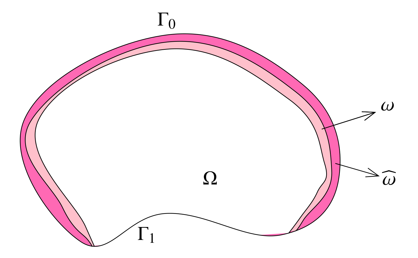
Figure 4. Example of the domain $\Omega$ with the partition of the boundary $(\Gamma_{0},\Gamma_{1})$ and the two neighborhood of the boundary $\widehat{\omega}$ and $\omega$.

Moreover, let us define $w(x,t):=\eta(x)v(x,t)$. It can be easily checked through the definition that the fractional Laplacian of $w$ is given by

$$(-\Delta)^{\,s}w=(-\Delta)^{\,s}(\eta v)=\eta(-\Delta)^{\,s}v+R$$

where $R$ is the reminder term

$$R:=v(-\Delta)^{\,s}\eta-c_{N,s}\,P.V.\int_{\mathbb{R}^{N}}\frac{(v(x,t)-v(y,t))(\eta(x)-\eta(y))}{|x-y|^{N+2s}}\,dy.$$ (4.14)

Therefore, this new function $w$ satisfies the equation

$$\begin{cases}iw_{t}+(-\Delta)^{\,s}w=R,&(x,t)\in Q\\ w\equiv 0,&(x,t)\in Q^{c}\\ w(x,0)=w_{0},&x\in\Omega.\end{cases}$$

In addition to that, following the procedure presented in [8], employing the definition of $R$, the fact that the function $\eta$ is regular (in particular, Lipschitz), and the classical Cauchy-Schwarz and Young’s inequalities, we can show that there exists a constant $\mathcal{B}>0$, not depending on $v$, such that

$${\left\|R(t)\right\|}_{H^{1-s}(\omega)}\leq\mathcal{B}{\left\|v(t)\right\|}_{H^{s}(\omega)}.$$ (4.15)

Now, starting from (4.1) applied to $w$, we have

$$\underbrace{\Gamma(1+s)^{2}\int_{\Sigma}\left(\frac{|w|}{\delta^{s}}\right)^{2}(x\cdot\nu)\,d\sigma dt}_{J}= \;s\int_{0}^{T}{\left\|(-\Delta)^{\,\frac{s}{2}}w(t)\right\|}_{L^{2}(\omega)}^{2}\,dt+\Im\int_{\omega}\overline{w}(x\cdot\nabla w)\,\big{|}_{0}^{T}\,dx$$

$$-\Re\int_{0}^{T}\int_{\omega}R\Big{(}N\overline{w}+2x\cdot\nabla\overline{w}\Big{)}\,dxdt.$$

Hence, applying the Cauchy-Schwarz inequality and (2.9), we obtain

$$J\leq\mathcal{C}\int_{0}^{T}{\left\|w(t)\right\|}_{H^{s}(\omega)}^{2}\,dt+\mathcal{C}\int_{0}^{T}{\left\|w(t)\right\|}_{L^{2}(\omega)}{\left\|R(t)\right\|}_{L^{2}(\omega)}\,dt+\mathcal{C}\int_{0}^{T}{\left\|w(t)\right\|}_{H^{s}(\omega)}{\left\|R(t)\right\|}_{H^{1-s}(\omega)}\,dt.$$

From (4.3), using Young’s inequality, and the fact that ${\left\|\cdot\right\|}_{L^{2}(\omega)}\leq{\left\|\cdot\right\|}_{H^{\beta}(\omega)}$ for any $\beta>0$, we get

$$J\leq\mathcal{C}\int_{0}^{T}{\left\|w(t)\right\|}_{H^{s}(\omega)}^{2}\,dt+\mathcal{C}\int_{0}^{T}{\left\|R(t)\right\|}_{H^{1-s}(\omega)}^{2}\,dt,$$

from which it is straightforward to obtain

$$J\leq\mathcal{C}\int_{0}^{T}{\left\|v(t)\right\|}_{H^{s}(\omega)}^{2}\,dt+\mathcal{C}\int_{0}^{T}{\left\|R(t)\right\|}_{H^{1-s}(\omega)}^{2}\,dt.$$

Finally, using (4.15), we obtain the estimate

$$J\leq\mathcal{C}\int_{0}^{T}{\left\|v(t)\right\|}_{H^{s}(\omega)}^{2}\,dt.$$

Hence, by using Theorem (4.3), the inequality (4.12) follows. ∎

Lemma 4.6.

Let $\Omega\subset\mathbb{R}^{N}$ be a bounded regular domain, $s\in(0,1)$, $f\in H^{-s}(\Omega)$, and let $v\in H_{0}^{s}(\Omega)$ be the solution of

$$\begin{cases}(-\Delta)^{\,s}v=f,&x\in\Omega,\\ v\equiv 0,&x\in\Omega^{c}.\end{cases}$$

Then, there exists a constant $\gamma>0$ such that

$${\left\|v\right\|}_{H^{s}(\widehat{\omega})}^{2}\leq\gamma\left[{\left\|f\right\|}_{H^{-s}(\omega)}^{2}+{\left\|v\right\|}_{L^{2}(\omega)}^{2}\right].$$ (4.17)

Proof.

Let us consider again the function $\eta(x)$ defined in (4.13) and let $w=\eta v$. Thus, $w$ satisfies

$$\begin{cases}(-\Delta)^{\,s}w=\eta f+R:=g,&x\in\omega,\\ w\in H^{s}_{0}(\omega),\end{cases}$$

where $R$ is the reminder term introduced in (4.14).

We recall that we have ${\left\|R\right\|}_{L^{2}(\omega)}<+\infty$. This, together with the assumption on $f$ and the definition of $\eta$, implies that $g\in H^{-s}(\omega)$. Thus, there exists some positive constant $\gamma$, independent of $g$, such that (see (2.5))

$${\left\|w\right\|}_{H^{s}(\omega)}^{2}\leq\gamma{\left\|g\right\|}_{H^{-s}(\omega)}^{2}.$$

Expanding this last expression we easily obtain the existence of another positive constant, that we will still note by $\gamma$, such that

$${\left\|w\right\|}_{H^{s}(\omega)}^{2} \leq\gamma\left[{\left\|f\right\|}_{H^{-s}(\omega)}^{2}+{\left\|v\right\|}_{L^{2}(\omega)}^{2}\,\right].$$

Hence, since

$${\left\|v\right\|}_{H^{s}(\widehat{\omega})}^{2}={\left\|w\right\|}_{H^{s}(\widehat{\omega})}^{2}\leq{\left\|w\right\|}_{H^{s}(\omega)}^{2},$$

we finally obtain the estimate (4.17). ∎

Lemma 4.7.

For any $T>0$ and $s\geq 1/2$, there exists a positive constant $\mathcal{C}$, depending only on $s$, $T$, $N$, $\Omega$ and $\omega$, such that for all $v$ solution of (1.5) it holds

$${\left\|v_{0}\right\|}_{H^{-s}(\Omega)}^{2}\leq\mathcal{C}\int_{0}^{T}{\left\|v(t)\right\|}_{H^{-s}(\omega)}^{2}\,dt.$$ (4.18)

Proof.

Let us define

$$\psi(x,t):=\int_{0}^{t}v(x,\tau)d\tau+\Theta(x),$$

where

$$\begin{cases}(-\Delta)^{\,s}\Theta=-iv_{0},&x\in\Omega,\\ \Theta\in H^{s}_{0}(\Omega).\end{cases}$$

It can be readily checked that $\psi$ is a solution of (1.5) with initial datum $\psi(x,0)=\Theta(x)$. Applying (4.12) to it we have

$${\left\|\Theta\right\|}_{H^{s}(\Omega)}^{2}\leq\mathcal{C}\int_{0}^{T}{\left\|\psi(t)\right\|}_{H^{s}(\omega)}^{2}\,dt$$

which, by elliptic regularity, and using (4.17), becomes

$${\left\|v_{0}\right\|}_{H^{-s}(\Omega)}^{2}\leq\mathcal{C}\int_{0}^{T}\left({\left\|\psi_{t}(t)\right\|}_{H^{-s}(\omega)}^{2}+{\left\|\psi(t)\right\|}_{L^{2}(\omega)}^{2}\,\right)\,dt.$$ (4.19)

From (4.19), proceeding by contradiction and using compactness, we finally obtain (4.18). ∎

Proof of Theorem 4.4.

First of all, recall that, from (4.12) and (4.18), we have

$${\left\|v_{0}\right\|}_{H^{s}_{0}(\Omega)}^{2}\leq\mathcal{C}\int_{0}^{T}{\left\|v(t)\right\|}_{H^{s}(\omega)}^{2}\,dt=\mathcal{C}\,{\left\|v\right\|}_{L^{2}(0,T;H^{s}(\omega))}^{2},$$ (4.20)

$${\left\|v_{0}\right\|}_{H^{-s}(\Omega)}^{2}\leq\mathcal{C}\int_{0}^{T}{\left\|v(t)\right\|}_{H^{-s}(\omega)}^{2}\,dt=\mathcal{C}\,{\left\|v\right\|}_{L^{2}(0,T;H^{-s}(\omega))}^{2}.$$ (4.21)

We are going to prove (4.11) by interpolation. To this end, let us consider the linear operator

$$\Lambda:H^{-s}(\Omega)\rightarrow L^{2}(0,T;H^{-s}(\omega))$$

defined by

$$\Lambda v_{0}:=\left.\left(e^{it(-\Delta)^{\,s}}v\right)\right|_{\omega}.$$

Clearly,

$${\left\|\Lambda v_{0}\right\|}_{L^{2}(0,T;H^{-s}(\omega))}\leq\mathcal{C}\,{\left\|v_{0}\right\|}_{H^{-s}(\Omega)}.$$

Furthermore, from (4.21) it follows that

$${\left\|\Lambda v_{0}\right\|}_{L^{2}(0,T;H^{-s}(\omega))}\geq\mathcal{C}\,{\left\|v_{0}\right\|}_{H^{-s}(\Omega)}.$$

Therefore, we can consider the closed subspace $X_{0}:=\Lambda(H^{-s}(\Omega))$ of $L^{2}(0,T;H^{-s}(\omega))$ and the linear operator $\Pi:=\Lambda^{-1}$ (since $\Lambda$ is an isomorphism between $H^{-s}(\Omega)$ and $X_{0}$). Thus,

$$\Pi\in\mathcal{L}(X_{0},Y_{0}),$$ (4.22)

with $Y_{0}:=H^{-s}(\Omega)$. If now we set $X_{1}:=X_{0}\cap L^{2}(0,T;H^{s}(\omega))$, it follows from (4.20) that

$$\Pi\in\mathcal{L}(X_{1},Y_{1}),$$ (4.23)

with $Y_{1}:=H^{s}(\Omega)$. From (4.22), (4.23) and [33, Theorem 5.1], we have $\Pi\in\mathcal{L}([X_{0},X_{1}]_{1/2},[Y_{0},Y_{1}]_{1/2})$. Moreover, [33, Lemma 12.1] yields $[Y_{0},Y_{1}]_{1/2}=L^{2}(\Omega)$ and from [4, Theorem 5.1.2] we conclude that

$$[L^{2}(0,T;H^{s}(\omega)),L^{2}(0,T;H^{-s}(\omega))]_{1/2}=L^{2}(0,T;[H^{s}(\omega);H^{-s}(\omega)]_{1/2})=L^{2}(0,T;L^{2}(\omega)).$$

Hence, since $X_{0}$ and $X_{1}$ are closed subspaces of $L^{2}(0,T;H^{-s}(\omega))$ and $L^{2}(0,T;H^{s}(\omega))$ respectively, using [33, Theorem 15.1] we can verify that the norm of the space $[X_{0},X_{1}]_{1/2}$ is equivalent to the norm of $L^{2}(0,T;L^{2}(\omega))$ and, since $\Pi\in\mathcal{L}([X_{0},X_{1}]_{1/2};L^{2}(\Omega))$, we finally obtain 4.11. ∎

Having proved the observability of (1.5) from a neighborhood of the boundary of the domain, our controllability theorem is now a direct consequence of a duality argument. This argument being classical (see, e.g., [13, 31, 32]) we are going to omit it here.

5. Conclusion and open problems and perspectives

In this paper, we have analyzed the interior controllability properties of a non-local Schrödinger-type equation involving the fractional Laplace operator $(-\Delta)^{\,s}$ on a bounded $C^{1,1}$ domain.

We firstly considered the one-dimensional case, and we employed spectral techniques to prove that the fractional Schrödinger equation is null controllable for $s\geq 1/2$, while for $s<1/2$ null controllability fails. Besides, when $s=1/2$ we showed that the null-controllability result holds true provided the time horizon $T$ is large enough.

These one-dimensional results have been then extended to the multi-dimensional case via the employment of multiplier techniques combined with the Pohozaev identity for the fractional Laplacian.

We conclude this work by briefly presenting some suggestions for open problems.

• Exterior controllability for the fractional Schrödinger equation.  The concept of exterior controllability for evolution equations involving the fractional Laplacian has been recently introduced in several contributions (see [1, 35, 55, 56, 57]). This is the equivalent of the boundary controllability property for local partial differential equations. It takes into account the non-locality of the fractional Laplacian, which yields the ill-posedness of boundary value problems associated to this operator. To the best of our knowledge, so far the exterior controllability property has been analyzed only in the context of fractional heat and wave equations. To consider the case of a fractional Schrödinger equation is then an interesting open problem.

• Micro-local analysis for the solutions of evolution equations with the fractional Laplacian.  Geometric Optics expansion for the solutions of an evolution PDE is a very powerful tool that, if well developed, can provide relevant information on the propagation of a wave-type equation and on the way in which its solutions interact with the boundaries or interfaces in the domain of definition (see, e.g. [40, 41]). This tool has also been applied, for instance in [3], to the study of controllability properties for different classes of partial differential equations. As far as we know, a complete analysis of micro-local properties of non-local models such as the ones we considered in this contribution has not been developed yet and it would then be an interesting research direction.

• Rigorous justification of the minimal controllability time in the case $s=1/2$.  In the proof of Theorem 4.3, when $s=1/2$, we introduced a minimal (strictly positive) time for (4.3) to hold. This came from the employment of (4.6) and from the fact that, if $s=1/2$, the spaces $H^{s}_{0}(\Omega)$ and $H^{1-s}_{0}(\Omega)$ clearly coincide and no compactness argument may be used. In particular, in this case, if $T$ is not large enough the constant in the lower estimate in (4.7) would be negative. Although this minimal time requirement may appear a technicality associated with our strategy for proving Theorem 4.3, we actually believe that this constraint cannot be removed. Indeed, through a simple stationary phase approach (see [58, Chapter 3]), it is possible to show that, for $s=1/2$, the velocity of propagation of the solution of (1.1) is finite (whereas it is infinite when $s>1/2$). By means of standard micro-local analysis techniques (see, e.g. [3]) one then expects that it is required a minimal positive time $T_{0}>0$ for the observability inequality (1.4) (hence, for the controllability of (1.1)) to hold. A rigorous justification of this simple observation is, to the best of our knowledge, still missing and represent a very interesting issue which deserves a deeper investigation.

References

- [1] H. Antil, U. Biccari, R. Ponce, M. Warma and S. Zamorano, Controllability properties from the exterior under positivity constraints for a 1-d fractional heat equation, arXiv preprint arXiv:1910.14529.
- [2] H. Antil, R. Khatri and M. Warma, External optimal control of nonlocal PDEs, Inverse Problems, 35.
- [3] C. Bardos, G. Lebeau and J. Rauch, Sharp sufficient conditions for the observation, control, and stabilization of waves from the boundary, SIAM J. Control Optim., 30 (1992), 1024–1065.
- [4] J. Bergh and J. Löfström, Interpolation spaces. An introduction, Berlin, 1976.
- [5] U. Biccari and V. Hernández-Santamarıa, Controllability of a one-dimensional fractional heat equation: theoretical and numerical aspects, IMA J. Math. Control Inf., 36 (2019), 1199–1235.
- [6] U. Biccari and M. Warma, Null-controllability properties of a fractional wave equation with a memory term., Evol. Eq. Control. Theo., 9 (2020), 399–430.
- [7] U. Biccari, M. Warma and E. Zuazua, Addendum: Local elliptic regularity for the Dirichlet fractional Laplacian, Adv. Nonlin. Stud., 17 (2017), 837–839.
- [8] U. Biccari, M. Warma and E. Zuazua, Local elliptic regularity for the Dirichlet fractional Laplacian, Adv. Nonlin. Stud., 17 (2017), 387–409.
- [9] U. Biccari, M. Warma and E. Zuazua, Controllability of the one-dimensional fractional heat equation under positivity constraints, Commun. Pure Appl. Anal., 19 (2020), 1949–1980.
- [10] M. Bologna, C. Tsallis and P. Grigolini, Anomalous diffusion associated with nonlinear fractional derivative Fokker-Planck-like equation: exact time-dependent solutions, Phys. Rev. E, 62 (2000), 2213.
- [11] T. Cazenave and A. Haraux, An introduction to semilinear evolution equations, vol. 13, Oxford University Press, 1998.
- [12] B. Claus and M. Warma, Realization of the fractional Laplacian with nonlocal exterior conditions via forms method, J. Evol. Equ., 20 (2020), 1597–1631.
- [13] J.-M. Coron, Control and nonlinearity, 136, American Mathematical Soc., 2009.
- [14] J. Dávila, M. Del Pino, S. Dipierro and E. Valdinoci, Concentration phenomena for the nonlocal Schrödinger equation with Dirichlet datum, Analysis & PDE, 8 (2015), 1165–1235.
- [15] J. Dávila, M. Del Pino and J. Wei, Concentrating standing waves for the fractional nonlinear Schrödinger equation, J. Differential Equations, 256 (2014), 858–892.
- [16] E. Di Nezza, G. Palatucci and E. Valdinoci, Hitchhiker’s guide to the fractional Sobolev spaces, Bull. Sci. Math., 136 (2012), 521–573.
- [17] S. Dipierro, G. Palatucci and E. Valdinoci, Dislocation dynamics in crystals: a macroscopic theory in a fractional Laplace setting, Commun. Math. Phys., 333 (2015), 1061–1105.
- [18] A. A. Dubkov, B. Spagnolo and V. V. Uchaikin, Lévy flight superdiffusion: an introduction, Internat. J. Bifur. Chaos, 18 (2008), 2649–2672.
- [19] A. Fiscella, R. Servadei and E. Valdinoci, Density properties for fractional Sobolev spaces, Ann. Acad. Sci. Fenn. Math, 40 (2015), 235–253.
- [20] C. G. Gal and M. Warma, Nonlocal transmission problems with fractional diffusion and boundary conditions on non-smooth interfaces, Comm. Partial Differential Equations, 42 (2017), 579–625.
- [21] G. Gilboa and S. Osher, Nonlocal operators with applications to image processing, Multiscale Model. Simul., 7 (2008), 1005–1028.
- [22] R. Gorenflo, F. Mainardi and A. Vivoli, Continuous-time random walk and parametric subordination in fractional diffusion, Chaos, Solitons Fractals, 34 (2007), 87–103.
- [23] G. Grubb, Fractional Laplacians on domains, a development of Hörmander’s theory of -transmission pseudodifferential operators, Adv. Math., 268 (2015), 478–528.
- [24] A. E. Ingham, Some trigonometrical inequalities with applications to the theory of series, Math. Z., 41 (1936), 367–379.
- [25] V. Komornik, Exact controllability and stabilization: the multiplier method, vol. 36, Masson, 1994.
- [26] T. Kulczycki, M. Kwaśnicki, J. Małecki and A. Stos, Spectral properties of the Cauchy process on half-line and interval, Proc. Lond. Math. Soc., pdq010.
- [27] M. Kwaśnicki, Eigenvalues of the fractional Laplace operator in the interval, J. Funct. Anal., 262 (2012), 2379–2402.
- [28] N. Laskin, Fractional quantum mechanics, Phys. Rev. E, 62 (2000), 3135.
- [29] N. Laskin, Fractional schrödinger equation, Phys. Rev. E, 66 (2002), 056108.
- [30] N. Laskin, Fractional quantum mechanics and Lévy path integrals, Phys. Letters A, 268 (2000), 298–305.
- [31] J. L. Lions, Contrôlabilité exacte perturbations et stabilisation de systèmes distribués(Tome 1, Contrôlabilité exacte. Tome 2, Perturbations), Recherches en mathematiques appliquées, Masson, 1988.
- [32] J.-L. Lions, Exact controllability, stabilization and perturbations for distributed systems, SIAM Rev., 30 (1988), 1–68.
- [33] J. L. Lions and E. Magenes, Problemes aux limites non homogenes et applications, Dunod, 1968.
- [34] S. Longhi, Fractional Schrödinger equation in optics, Optics letters, 40 (2015), 1117–1120.
- [35] C. Louis-Rose and M. Warma, Approximate controllability from the exterior of space-time fractional wave equations, Appl. Math. Optim., 1–44 (2018).
- [36] B. B. Mandelbrot and J. W. Van Ness, Fractional Brownian motions, fractional noises and applications, SIAM Rev., 10 (1968), 422–437.
- [37] M. M. Meerschaert, Fractional calculus, anomalous diffusion, and probability, in Fractional Dynamics: Recent Advances, World Scientific, 2012, 265–284.
- [38] S. Micu and E. Zuazua, An introduction to the controllability of partial differential equations, in Quelques questions de théorie du contrôle, Sari, T., ed., Collection Travaux en Cours Hermann, 2004.
- [39] S. I. Pohozaev, On the eigenfunctions of the equation , Soviet Math. Dokl, 6 (1965), 1408–1411.
- [40] J. Ralston, Gaussian beams and the propagation of singularities, Studies in partial differential equations, 23 (1982), C248.
- [41] J. Rauch, X. Zhang and E. Zuazua, Polynomial decay for a hyperbolic-parabolic coupled system, J. Math. Pures Appl., 84 (2005), 407–470.
- [42] X. Ros-Oton and J. Serra, The Dirichlet problem for the fractional Laplacian: regularity up to the boundary, J. Math. Pures Appl., 101 (2014), 275–302.
- [43] X. Ros-Oton and J. Serra, The extremal solution for the fractional Laplacian, Calc. Var. Partial Differential Equations, 50 (2014), 723–750.
- [44] X. Ros-Oton and J. Serra, The Pohozaev identity for the fractional Laplacian, Arch. Rat. Mech. Anal., 213 (2014), 587–628.
- [45] R. Servadei and E. Valdinoci, Variational methods for non-local operators of elliptic type, Discrete Contin. Dyn. Syst, 33 (2013), 2105–2137.
- [46] R. Servadei and E. Valdinoci, On the spectrum of two different fractional operators, Proc. Roy. Soc. Edinburgh Sect. A, 144 (2014), 831–855.
- [47] R. Servadei and E. Valdinoci, A Brezis-Nirenberg result for non-local critical equations in low dimension, Comm. Pure Appl. Anal., 12 (2013), 2445–2464.
- [48] J. Simon, Compact sets in the space , Ann. Mat. Pura Appl., 146 (1986), 65–96.
- [49] B. Stickler, Potential condensed-matter realization of space-fractional quantum mechanics: the one-dimensional Lévy crystal, Phys. Rev. E, 88 (2013), 012120.
- [50] M. Tucsnak and G. Weiss, Observation and control for operator semigroups, Springer Science & Business Media, 2009.
- [51] E. Valdinoci, From the long jump random walk to the fractional Laplacian, Bol. Soc. Esp. Mat. Apl. SeMA, 49 (2009), 33–44.
- [52] J. L. Vázquez, Nonlinear diffusion with fractional Laplacian operators, in Nonlinear partial differential equations, Springer, 2012, 271–298.
- [53] G. M. Viswanathan, V. Afanasyev, S. Buldyrev, E. Murphy, P. Prince and H. E. Stanley, Lévy flight search patterns of wandering albatrosses, Nature, 381 (1996), 413.
- [54] M. Warma, The fractional relative capacity and the fractional Laplacian with Neumann and Robin boundary conditions on open sets, Potential Anal., 42 (2015), 499–547.
- [55] M. Warma, Approximate controllability from the exterior of space-time fractional diffusive equations, SIAM J. Control Optim., 57 (2019), 2037–2063.
- [56] M. Warma and S. Zamorano, Null controllability from the exterior of a one-dimensional nonlocal heat equation, Control & Cybernetics, 48 (2019), 417–438.
- [57] M. Warma and S. Zamorano, Analysis of the controllability from the exterior of strong damping nonlocal wave equations, ESAIM: Control Optim. Calc. Var., 26 (2020), 42.
- [58] G. B. Whitham, Linear and nonlinear waves, vol. 42, John Wiley & Sons, 1999.
- [59] K. Yosida, Functional analysis, vol. 6, Springer-Verlag, Berlin New York, 1980.