Flying Objects Detection from a Single Moving Camera

Abstract

We propose an approach to detect flying objects such as UAVs and aircrafts when they occupy a small portion of the field of view, possibly moving against complex backgrounds, and are filmed by a camera that itself moves.

Solving such a difficult problem requires combining both appearance and motion cues. To this end we propose a regression-based approach to motion stabilization of local image patches that allows us to achieve effective classification on spatio-temporal image cubes and outperform state-of-the-art techniques.

As the problem is relatively new, we collected two challenging datasets for UAVs and Aircrafts, which can be used as benchmarks for flying objects detection and vision-guided collision avoidance.

1 Introduction

We are headed for a world in which the skies are occupied not only by birds and planes but also by unmanned drones ranging from relatively large Unmanned Aerial Vehicles (UAVs) to much smaller consumer ones. Some of these will be instrumented and able to communicate with each other to avoid collisions but not all. Therefore, the ability to use inexpensive and light sensors such as cameras for collision-avoidance purposes will become increasingly important.

This problem has been tackled successfully in the automotive world and there are now commercial products [9, 16] designed to sense and avoid both pedestrians and other cars. In the world of flying machines most of the progress is achieved in the accurate position estimation and navigation from single or multiple cameras [4, 14, 15, 8, 25, 13, 7], while not so much is done in the field of visual-guided collision avoidance [27]. On the other hand, it is not possible to simply extend the algorithms used for pedestrian and automobile detection to the world of aircrafts and drones, as flying object detection poses some unique challenges:

• The environment is fully 3D dimensional, which makes the motions more complex.

• Flying objects have very diverse shapes and can be seen against either the ground or the sky, which produces complex and changing backgrounds, as shown in Fig. 1.

• Given the speeds involved, potentially dangerous objects must be detected when they are still far away, which means they may still be very small in the images.

As a result, motion cues become crucial for detection. However, they are difficult to exploit when the images are acquired by a moving camera and feature backgrounds that are difficult to stabilize because they are non-planar and fast changing. Furthermore, since there can be other moving objects in the scene, for example, the person in Fig. 1, motion by itself is not enough and appearance must also be taken into account. In these situations, state-of-the-art techniques that rely on either image flow or background stabilization lose much of their effectiveness.

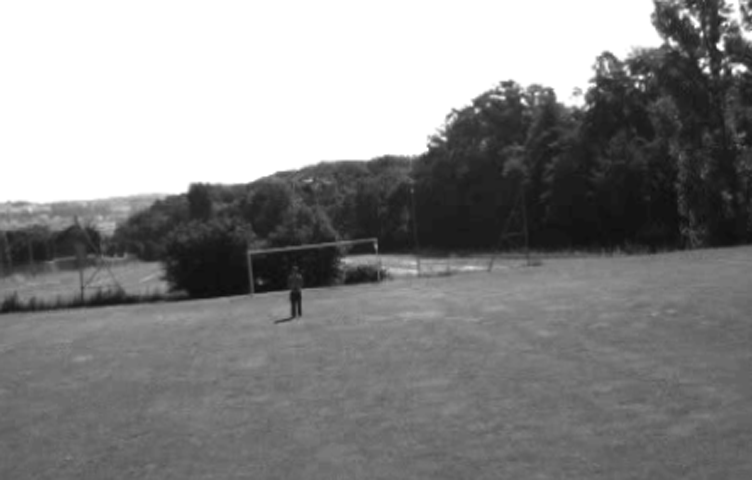
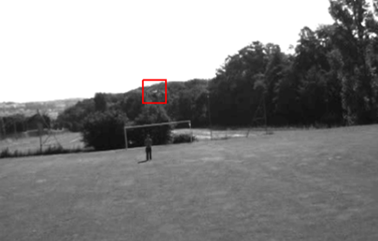
Figure 1: Detecting a small drone against a complex moving background. (Left) It is almost invisible to the human eye and hard to detect from a single image. (Right) Yet, our algorithm can find it by using motion clues.

In this paper, we detect whether an object of interest is present and constitutes a danger by classifying 3D descriptors computed from spatio-temporal image cubes. We will refer to them as st-cubes. These st-cubes are formed by stacking motion-stabilized image windows over several consecutive frames, which gives more information than using a single image. What makes this approach both practical and effective is a regression-based motion-stabilization algorithm. Unlike those that rely on optical flow, it remains effective even when the shape of the object to be detected is blurry or barely visible, as illustrated by Fig. 2.

St-cubes of image intensities have been routinely used, for action recognition purposes [10, 24] using a single fixed camera. In contrast, most current detection algorithms work on a single frame, or integrate the information from two of them, which might not be consecutive, by taking into account optical flow from one frame to another. Our approach can therefore be seen as a way to combine both the appearance and motion information to achieve effective detection in a very challenging context.

2 Related work

Approaches to detecting moving objects can be classified into three main categories, those that rely on appearance in individual frames, those that rely primarily on motion information across frames, and those that combine the two. We briefly review all three types in this section. In the results section, we will demonstrate that we can outperform state-of-the-art representatives of each.

Appearance-based methods rely on Machine Learning and have proved to be powerful even in the presence of complex lighting variations or cluttered background. They are typically based on Deformable Part Models (DPM) [6], Convolutional Neural Networks (CNN) [19] and Random Forests [1]. We will evaluate our approach in comparison with all of these methods and the another, which relies on an Aggregate Channel Features (ACF) [5], as it is widely considered to be among the best.

However, they work best when the target objects are sufficiently large and clearly visible in individual images, which is often not the case in our applications. For example, in the image of Fig. 1, the object is small and it is almost impossible to make out from the background without motion cues.

Motion-based approaches can themselves be subdivided into two subclasses. The first comprises those that rely on background subtraction [17, 20, 21] and detect objects as groups of pixels that are different from the background. The second includes those that depend on optical flow between consecutive images [3, 12]. Background subtraction works best when the camera is static or its motion is small enough to be easily compensated for, which is not the case for the on-board camera of a fast moving vehicle. Flow-based methods are more reliable in such situations but are critically dependent on the quality of the flow vectors, which tends to be low when the target objects are small and blurry.

Hybrid approaches combine information about object appearance and motion patterns and are therefore closest in spirit to what we propose. For example, in [23], histograms of flow vectors are used as features in conjunction with more standard appearance features and fed to a statistical learning method. This approach was refined in [18] by first aligning the patches to compensate for motion and then using the differences of frames that may or may not be consecutive as additional features. The alignment relies on the Lucas-Kanade optical flow algorithm [12]. The resulting algorithm works very well for pedestrian detection and outperforms most of the single-frame ones. However when the target objects become smaller and harder to see, the flow estimates become unreliable and this approach, like the purely flow-based ones, becomes less effective.

3 Approach

UAVs

Aircrafts

Uniform background

Very noisy background

Non-uniform background

Noisy background

No motion compensation

Lucas-Kanade optical flow

Our approach

(a)

(b)

(c)

(d)

Figure 2: Compensation for the apparent motion of different flying objects inside the st-cube allows to decrease in-class variation of the data, used by the machine learning algorithms. For each st-cube, we also provide three graphs: The blue dots in the first graph indicate the locations of the center of the drone throughout the st-cube, the red cross indicates the patch center. The next two graphs plot the variations of the $x$ and $y$ coordinates of the center of the drone respectively, compared to the position of the center of the patch. We can see that our method keeps the drone close to the center even for complicated backgrounds and when the drone is barely recognizable as in the right column.

In this section, we first introduce a basic approach to using st-cubes, that is, blocks of consecutive frames, for object detection without first correcting for motion. We then introduce our regression-based approach to motion stabilization. We will demonstrate in the result section that it brings a substantial performance improvement.

3.1 Detection without Motion Stabilization

Let $s_{x}$ and $s_{y}$ be spatial, and $s_{t}$ be temporal dimensions of a st-cube such as those depicted by Fig. 3. We use a training set of pairs $(b_{i},y_{i}),i\in[1,N]$, where $b_{i}\in R^{s_{x}\times s_{y}\times s_{t}}$ is a st-cube and the label $y_{i}\in[-1,1]$ indicates whether or not it contains a target object. We then train an AdaBoost classifier:

$$F:\mathbb{R}^{s_{x}\times s_{y}\times s_{t}}\rightarrow[0,1],\qquad F(b)=\mathop{\Sigma}\limits_{j=1}^{T}\alpha_{j}f_{j}(b)$$ (1)

where the $\alpha_{j}$ are learned weights and $T$ is the number of weak classifiers $f_{j}$ learned by the algorithm. We use $f_{j}$ of the form

$$f_{R,o,\tau}(b)=\left\{\begin{array}[]{ll}1&\text{ if }E(b,R,o)>\tau,\\ 0&\text{ otherwise.}\\ \end{array}\right.$$ (2)

These weak learners are parametrized by a box $R$ within $b$, an orientation $o$ and a threshold $\tau$. $E(b,R,o)$ is the normalized image gradient energy at orientation $o$ over the region $R$ [11].

As a potential alternative to these image features, we tested a 3D version of the HOG detector as in [24]. However, we found that its performance depends critically on the size of the bins used to compute it. In practice, we found it difficult to find sizes that consistently gave good results for objects whose apparent shape can change dramatically. The AdaBoost procedure solves this problem by automatically selecting an appropriate range of sizes of the boxes $R$ of Eq. 2.

One problem the AdaBoost procedure does not address, however, is that the orientations of the gradients are biased by the global object motion and that this bias is independent of object appearance. This makes the learning task much more difficult and motion stabilization is required to eliminate this problem.

3.2 Object-Centric Motion Stabilization

mUAVs			Aircrafts

Figure 3: Sample patches of the mUAVs and aircrafts. Each column corresponds to a single st-cube and illustrates one kind from the variety of possible motions that an aircraft could have.

The best way to avoid the above-mentioned bias is to guarantee that the target object, if present in an st-cube, remains at the center of all spatial slices.

More specifically, let $I_{t}$ denote the $t^{th}$ frame of the video sequence. If we do not compensate for the motion, we can define the st-cube $b_{i,j,t}$ as the 3-D array of pixel intensities from $I_{z},z\in[t-s_{t}+1,t]$ at image locations $(k,l),k\in[i-s_{x}+1,i],l\in[j-s_{y}+1,j]$, as depicted by Fig. 3. Given these notations, correcting for motion can be formulated as allowing the $s_{t}$ spatial slices $m_{i,j,z},z\in[t-s_{t}+1,t]$ to shift horizontally and vertically in individual images.

In [18], these shifts are computed using flow information, which has been shown to be effective in the case of pedestrians who occupy a large fraction of the image and move relatively slowly from one frame to the next. However, as can be seen in Fig. 3 these assumptions do not hold in our case and we will show in the result section that this negatively impacts the performance.

To overcome this difficulty, we introduce instead a regression-based approach to compensate for motion and keep the object in the center of the $m_{i,j,z}$ spatial slices even when the target object’s appearance changes drastically.

Training the regressors

We propose to train two boosted trees regressors [22], one for horizontal motion of the aircraft and one for its vertical motion. The power of this method is that it does not use the similarity between consecutive frames, and is able to predict how far the object is from the center in the horizontal or vertical directions, based just on a single patch.

We use gradient boosting [26] to learn regression models for vertical $\phi_{v}(\cdot)$ and horizontal motion $\phi_{h}(\cdot)$. Each of these models $\phi_{*}:\mathbb{R}^{s_{x}\times s_{y}}\rightarrow\mathbb{R}$ can be represented in the form $\phi_{*}(m)=\mathop{\Sigma}_{j=1}^{T}\alpha_{j}h_{j}(m)$, where $\alpha_{j=1..T}$ are real valued weights, $h_{j}:\mathbb{R}^{s_{x}\times s_{y}}\rightarrow\mathbb{R}$ are weak learners and $m\in\mathbb{R}^{n}$ is the input patch. The GradientBoost approach can be seen as extension of the classic AdaBoost algorithm to real-valued weak learners and more general loss functions.

As typically done with gradient boosting we use regression trees $h_{j}(m)=T(\theta_{j},HoG(m))$ as weak learners for this approach, where $\theta_{j}$ denotes the tree parameters. $HoG(m)$ denotes the Histograms of Gradients for patch $m$. At every iteration $j$ the boosting approach finds the weak learner $h_{j}(\cdot)$ that minimises the quadratic loss function

$$h_{j}(\cdot)=\mathop{argmin}\limits_{h(\cdot)}\left(\mathop{\Sigma}\limits_{i=1}^{N}w_{i}^{j}(h(x_{i})-r_{i})^{2}\right),$$ (3)

where $N$ is the number of training samples $m_{i}$ with their expected responses $r_{i}$. Weights $w_{i}^{j}$ are estimated at every iteration, by differentiating the loss function.

We used the $HoG(\cdot)$ representation for the patches $m_{i=1..N}$ because it is fast to compute and proved to be robust to illumination changes in many applications. Therefore the regressor is able to perform in the outdoor environments, where illumination can significantly change from one part of the video sequence to another.

Motion compensation with regression

After both regressors for horizontal and vertical motions are trained, we use them to compensate for the motion of the aircraft inside the st-cube $b_{i,j,t}$ in an iterative way. Algorithm 1 outlines the main steps the motion compensation approach takes to estimate and correct for the shift of the aircraft. The resulting st-cube keeps the aircraft close to the center throughout the whole sequence of patches $m_{k=1..s_{t}}$ of $b_{i,j,t}$. This approach provides not only a better prediction, but also allows to estimate the direction of motion of the aircraft and its speed, provided the frame-rate of the camera and the size of the target object are known. This additional information may be used by various tracking algorithms to improve their performance.

Algorithm 1 Regression based motion compensation.

  Input

  

1. regressors $\phi_{h}(\cdot),\phi_{v}(\cdot)$ for horizontal and vertical motion respectively

2. st-cube $b_{i,j,t}$ with dimensions $s_{x},s_{y},s_{t}$

3. frames $I_{p},p\in[t-s_{t}+1,t]$ of the video sequence

  

  set $\epsilon=1$

  for $m_{k},k\in[1,s_{t}]$ do

     set $n=1$, $(i_{0},j_{0})=(0,0)$ and $(i_{1},j_{1})=(i,j)$

     

     as it was previously defined, we refer to $m_{k}$ as the patch of the st-cube and to $m_{i,j,p},p=k+t-s_{t}$ as the patch extracted from the $I_{p}$ at the position $(i,j)$, so at the first iteration $m_{k}=m_{i_{1},j_{1},p}$

     

     while $\left((i_{n}-i_{n-1})^{2}+(j_{n}-j_{n-1})^{2}\right)<\epsilon$ do

        $n=n+1$

        $(sh_{h},sh_{v})=\left(\phi_{h}(m_{p}),\phi_{v}(m_{p})\right)$

        $(i_{n},j_{n})=(i_{n-1}-sh_{v},j_{n-1}-sh_{h})$

        $m_{k}=m_{i_{n},j_{n},p}$

     end while

  end for

Fig. 2 show examples of st-cubes before and after motion compensation for different flying objects. For each of the st-cubes $b$ and for each patch $m_{k=1..s_{t}}$ inside $b$ we plot the position of the actual center of the flying object with respect to the center of the patch.

We can see from these examples that the optical flow approach is more focused on the background, as in the case where the background is not uniform, the positions of the drone over the patches are spread across the patch. However, in the case of our regression-based motion compensation the center positions of the drone are located close to each other and to the center of the patch. Moreover if the appearance of the drone changes inside the st-cube (e.g. due to the lighting changes) optical flow based method is unable to correctly estimate the shift of the object. On the other hand our regression approach is capable of identifying the correct shift even in the situations when the outlines of the object are heavily corrupted by noise, coming from the background. Fig. 2 illustrates this fact for different flying objects and various background complexity levels. Note also that our regressor generalizes well to different objects that were not used for training.

Provided regressors are estimated, we use them for motion compensation of the flying objects inside the st-cubes of the training dataset. This allows us to train the AdaBoost classifier from Eq. 1, on the data with much less in-class variation and thus it is easier for the machine learning algorithm to fit a proper model to it.

Original frames from the video sequences
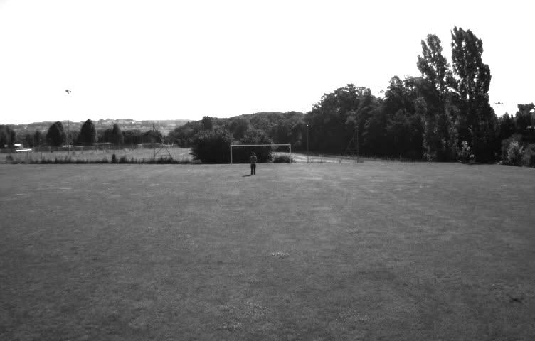
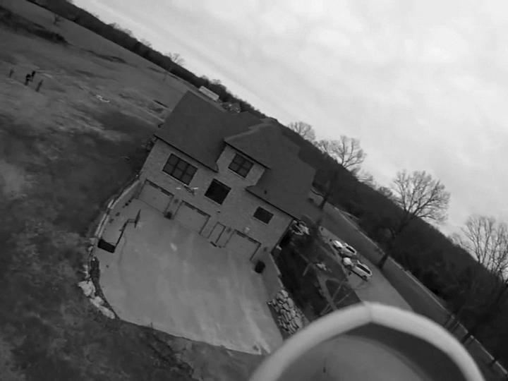
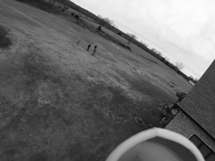
Background subtraction
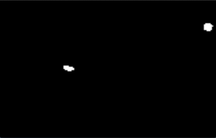
Optical flow
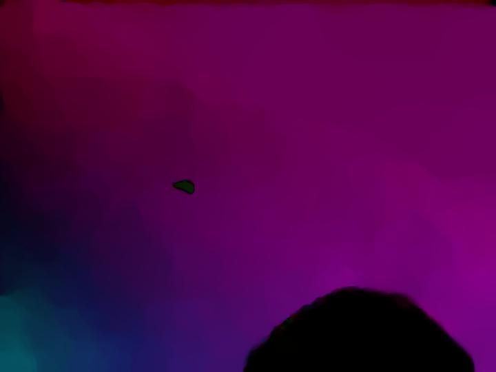
Our approach
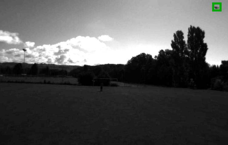
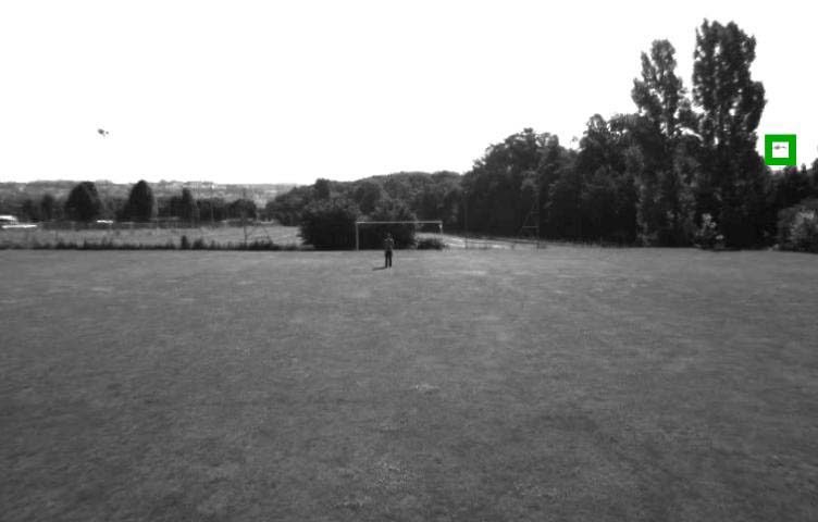
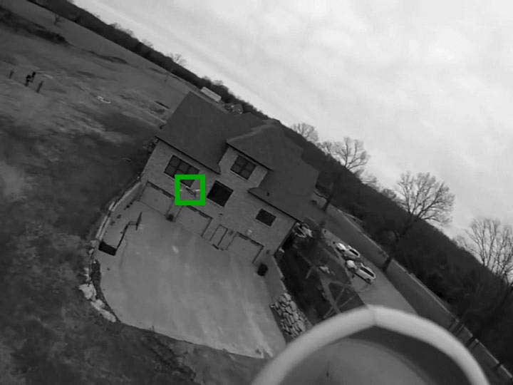
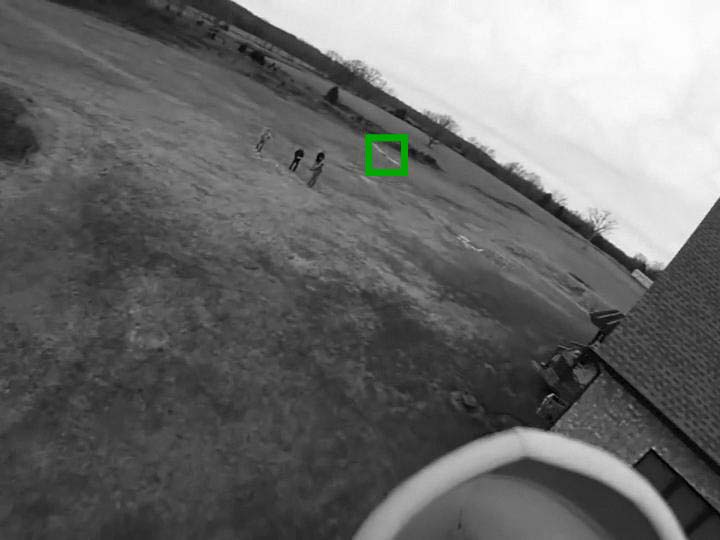
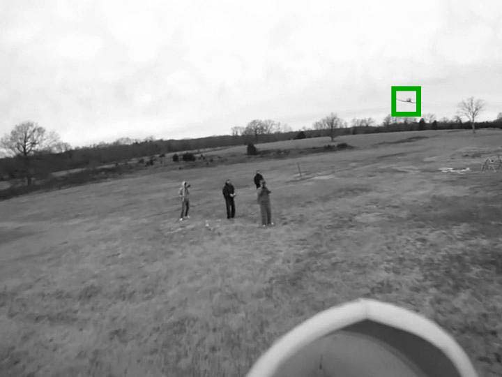
UAV dataset				Aircraft dataset

Figure 4: Comparison of our approach with motion-based methods. First row: Original frames from the video sequences. Second row: Using a state-of-the art subtraction algorithm [20] is not sufficient to detect the target objects as the camera is moving and the background can vary because of trees and grass moving with the wind. The UAV is detected only in one image, together with a false detection. The plane is detected in only one image as well, together with large errors. Third row: The task is also very difficult for a state-of-the-art optical flow approach [3]. The UAV is not revealed in the optical flow images, the plane is visible in only two of them. Bottom row: Our detector can detect the target objects by relying on motion and appearance. (best seen in color)

4 Results

In this section, we evaluate the performance of our approach against state-of-the-art ones [5, 18] on two challenging datasets. They include many real-world challenges such as fast illumination changes and complex backgrounds, created by moving treetops seen against a changing sky. They are as follows:

(a) UAV dataset				(b) Aircraft dataset

Figure 5: Sample image windows containing aircrafts or UAVs from our datasets.

• UAV dataset It comprises 20 video sequences of 4000 $752\times 480$ frames each on average. They were acquired by a camera mounted on a drone filming similar ones while flying outdoors. As can be seen in Fig. 5(a), there appearance is extremely variable due to changing attitudes and lighting conditions.

• Aircraft dataset It consists of 20 YouTube videos of planes or radio controlled plane-like drones. Some videos were acquired by a camera on the ground and the rest was filmed by a camera on board of an aircraft. These videos vary in length from hundreds to thousands of frames and in resolution from $640\times 480$ to $1280\times 720$. Fig. 5(b) depicts the variety of plane types that can be seen in them.

We will make these datasets, together with the ground-truth annotations, publicly available as a new challenging benchmark for aerial objects detection and visual-guided collision avoidance.

4.1 Training and Testing

In all cases we used half of the data to train both the regressor of Eq. 3 and the classifier of Eq. 1. We manually supplied 8000 bounding boxes centered on a UAV and 4000 on a plane.

Training the Regressors

To provide labeled examples, where the aircraft or UAV is not in the center of the patch but still at least partially within it, we randomly shifted the manually supplied bounding boxes by distances of up to half of their size. This step is repeated for every second frame of the training database to cover the variety of shapes and backgrounds in front of which the aircraft might appear.

The apparent size of the objects in the UAV and Aircraft datasets vary from 10 to 100 pixels on the image plane. To train the regressor, we used $40\times 40$ patches containing the UAV or aircraft shifted from the center. We have chosen this size because smaller ones will result in fewer features available for gradient boosting, while bigger ones will introduce noise and take more time to analyze. We detect the targets at different scales by running the detector on the image at different resolutions.

Training the Classifiers

We used the st-cubes of size $(s_{x},s_{y},s_{z})=(40,40,4)$, the spatial dimensions being the same as for regression. The choice of $s_{z}=4$ represents a compromise between being able to detect far away objects by increasing $s_{z}$ and closer ones that require a smaller $s_{z}$ because the frame-to-frame motion might be too big for our motion-compensation mechanism.

Evaluation Metric

We report precision-recall curves. Precision is computed as the number of true positives, detected by the algorithm divided by the total number of detections. Recall is the number of true positives divided by the number of the positively labeled test examples. Additionally we use the Average Precision (AveP) measure, which we take to be the integral $\int_{0}^{1}p(r)dr$, where $p$ is the precision, and $r$ the recall.

4.2 Baselines

To demonstrate the effectiveness of our approach, we compare it against state-of-the-art algorithms. We chose them to be representative of the three different ways the problem of detecting small moving objects can be approached, as discussed in Section 2.

• Appearance-Based Approaches that rely on detection in individual frames. We will compare against Deformable Part Models (DPMs) [6], Convolutional Neural Networks (CNN) [19], Random Forests [2], and Aggregate Channel Features method (ACF) [5], the latter being widely considered to be among the best. Since our algorithm labels st-cubes as positive or negative, for a fair comparison with these single frame algorithms, we proceed as follows. If they label the middle frame of the cube as positive, then the whole st-cube is regarded as a positive detection and otherwise not.

• Motion-based Approaches do not use any appearance information and rely purely on the correct estimation of the background motion. Among those we experimented with MultiCue background subtraction [20, 21] and large displacement optical flow [3].

• Hybrid approaches are closest in spirit to ours and correct for motion using image-flow. Among those, the one presented in [18] is the most recent one we know of and the one we compare against. To ensure fair comparison, we used the same size st-cubes for both.

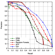
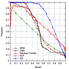
UAV dataset	Aircraft dataset

Figure 6: Comparison against apperance-based approaches. For both the UAV and Aircraft datasets, our approach achieves about a $10\%$ increase of performance compared to the state-of-the-art ACF method.

	Average Precision
Method	UAV dataset	Aircraft dataset
DPM [6]	0.573	0.470
CNN [19]	0.504	0.547
Random Forests [2]	0.618	0.563
ACF [5]	0.652	0.648
St-cubes without	0.485	0.497
motion compensation
St-cubes+optical flow	0.540	0.652
Park [18]	0.568	0.705
Our	0.751	0.789

Table 1: Average precision of detection methods on our datasets. We can see that in both cases our approach with regression-based motion compensation is able to outperform both purely appearance based methods and state-of-the-art hybrid approach.

4.3 Evaluation against Competing Approaches

Here we compare our regression-based approach against the three classes of methods discussed above.

Appearance-Based Methods.

Fig. 6 compares our method with appearance-based approaches on our two datasets. Table 1 summarizes the results in terms of Average Precision. For both the UAV and Aircraft datasets we can achieve on average around $10\%$ improvement, in terms of this measure, over the ACF method, which itself outperforms the others. The DPM and CNN methods perform the worst on average. Most likely, this happens because the first one depends on using the correct size of the bins for HoG estimation, which makes it hard to generalize for a large variety of flying objects and the second one requires much more training samples than our detector does.

Motion-Based Methods.

Fig. 4 shows that state-of-the-art background subtraction [20] and optical flow computation [3] do not work well enough for detecting UAVs or planes in the challenging conditions that we consider.

We do not provide precision-recall curves for motion-based methods because it it not clear how big the moving part of the frame should be to be considered as an aircraft. We have tested several potential sizes and the average precision was much lower than those in Table 1 in all cases.

Motion compensation approaches.

Fig. 7 compares our motion compensation algorithm with the optical flow-based one used in [18] for both UAV and Aircraft datasets. Using motion compensation for alignment of the st-cubes results into higher performance of the detectors, as the in-class variation of the data is decreased. Table 1 shows that we can achieve at least $15\%$ improvement in average precision on both datasets using our motion compensation algorithm.

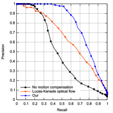
(a) UAV dataset	(b) Aircraft dataset

Figure 7: Evaluation of the motion compensation methods on our datasets. Unlike other motion compensation algorithms, our regression-based method is able to properly identify the shift in object position and correct for it, even in the situation, when the background is complex and the outlines of the object are barely visible, which leads to significant improvement in the detection accuracy.

Among the motion compensation approaches our regression-based method outperforms the optical flow-based one of [18], because it is able to correctly compensate for the mUAV motion even in the cases where the background is complex and the drone might not be visible even to the human eye. Fig. 2(b,d) illustrates this hard situation with an example. On the contrary, the optical flow method is more focused on the background, which decreases its performance. Fig. 2(b) shows an example of a relatively easy situation, when the aircraft is clearly visible, but the optical flow algorithm fails to correctly compensate for its shift from the center, while our regression-based approach succeeds.

Our regression-based motion compensation algorithm allows us to significantly reduce the in-class variation of the data, which results into $30\%$ boost in performance, as given by the Average precision measure.

Hybrid approaches.

Fig. 8 illustrates the comparison of our method to the hybrid approach [18], which relies on motion compensation using Lucas-Kanade optical flow method, and yields state-of-the-art performance for pedestrian detection. For both UAV and Aircraft datasets our method is able to achieve higher performance, due to our regression-based approach for compensating motion that allows to properly identify and correct for the shift of the aircraft inside the block of patches, used for detection.

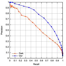
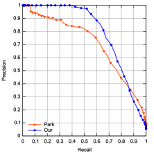
(a) UAV dataset	(b) Aircraft dataset

Figure 8: Comparison of our approach to the hybrid method (Park). Our method is able to show higher performance for both of the datasets, due to the regression-based motion compensation algorithm used.

4.4 Collision Courses

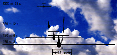
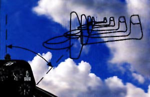
Figure 9: Collision courses. (Left) The apparent size of a standard glider and its 15 m wingspan flying towards another aircraft at a relatively slow speed (100 km/h) is very small 33s before impact, but the glider completely fills the field of view only half a minute later, 3s before impact. (Right) An aircraft on a collision course is seen in a constant direction but its apparent size grows, slowly at first and then faster.

Detecting another aircraft on a potential collision course is an important sub-case of the more generic detection problem we are addressing in this paper. As shown in Fig. 9(b), the hallmark of a collision course is that the object on such a course is always seen at a constant angle and that its size increases slowly, at least at first.

This means that motion stabilization is less important in this case and that the temporal gradients have a specific distribution. In other words, the in-class variation for the positive examples should be much smaller in this scenario than in the general case and could be potentially be captured by a 3D HoG descriptor [24]. This gives us a good way to test whether our motion-stabilization mechanism negatively impacts performance in this specific case, as do most mechanisms that enforce invariance when such invariance is not required.

To this end, we therefore searched YouTube for a set of video sequences in which airplanes appear to be on a collision course for substantial amount of time. We selected 14 videos that vary in length from tens to several hundreds of frames. As before, we used half of them for training the collision course detector and the other to test it. In Fig. 10, we compare our results against those obtained using classification based on a 3D HoG descriptor [24] without motion compensation, as suggested above. This corresponds to the method labeled “St-cubes without motion compensation” in Table 1. As expected, even though it did not perform very well in the general case, it turns out to be very effective in this specific scenario. Our approach is very slightly less precise, which reflects the phenomenon discussed above.

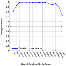
AveP Detector: (Average Precision) 3D HOG 0.907 Our 0.904

Figure 10: Performance for aircrafts on a collision course. (Top) Distribution of the average precision we can achieve as a function of the size of the aircraft in the video frame. It is close to 100% for sizes between 35 pixels and 75 pixels, which translates to a useful range of distances for collision avoidance purposes. (Bottom) The Average Precision of our method compared to using a 3D HOG detector.

Furthermore, the curve at the top of Fig. 10 shows that it is only when the aircraft is either very small in the image ($<30$ pixels) or very close that the average precision of our detector slightly decreases. In the first case, this happens because the object is too far and the increase of its apparent size is hardly perceptible. In the second case, the appearance changes very significantly for different types of aircrafts, which harms performance. However the goal of a collision avoidance system is to avoid these kinds of situations and to detect the aircraft at a safe distance. We can see that our approach allows us to achieve close to $100\%$ performance within a large range and could therefore be used for this purpose.

5 Conclusion

We showed that temporal information from a sequence of frames plays a vital role in detection of small fast moving objects like UAVs or aircrafts in complex outdoor environments. We therefore developed an object-centric motion compensation approach that is robust to changes of the appearances of both the object and the background. This approach allows us to outperform state-of-the-art techniques on two challenging datasets. Motion information provided by our method has a variety of applications, from detection of potential collision situations to improvement of vision-guided tracking algorithms.

We collected two challenging datasets for UAVs and Aircrafts. These datasets can be used as a new benchmark for flying objects detection and visual-based aerial collision avoidance.

References

- [1] A. Bosch, A. Zisserman, and X. Munoz. Image Classification Using Random Forests and Ferns. In International Conference on Computer Vision, 2007.
- [2] L. Breiman. Random Forests. Machine Learning, 2001.
- [3] T. Brox and J. Malik. Large displacement optical flow: descriptor matching in variational motion estimation. IEEE Transactions on Pattern Analysis and Machine Intelligence, 2011.
- [4] G. Conte and P. Doherty. An Integrated UAV Navigation System Based on Aerial Image Matching. In IEEE Aerospace Conference, pages 3142–3151, 2008.
- [5] P. Dollár, Z. Tu, P. Perona, and S. Belongie. Integral Channel Features. In British Machine Vision Conference, 2009.
- [6] P. Felzenszwalb, R. Girshick, D. McAllester, and D. Ramanan. Object Detection with Discriminatively Trained Part Based Models. IEEE Transactions on Pattern Analysis and Machine Intelligence, 32(9), 2010.
- [7] C. Forster, M. Pizzoli, and D. Scaramuzza. SVO: Fast Semi-Direct Monocular Visual Odometry. In International Conference on Robotics and Automation, 2014.
- [8] C. Hane, C. Zach, J. Lim, A. Ranganathan, and M. Pollefeys. Stereo depth map fusion for robot navigation. In Proceedings of International Conference on Intelligent Robots and Systems, pages 1618–1625, 2011.
- [9] Mercedes-Benz Intelligent Drive. http://techcenter.mercedes-benz.com/en/intelligentdrive/detail.html/.
- [10] I. Laptev. On space-time interest points. International Journal of Computer Vision, 64(2-3):107–123, 2005.
- [11] K. Levi and Y. Weiss. Learning Object Detection from a Small Number of Examples: the Importance of Good Features. In Conference on Computer Vision and Pattern Recognition, 2004.
- [12] B. Lucas and T. Kanade. An Iterative Image Registration Technique with an Application to Stereo Vision. In International Joint Conference on Artificial Intelligence, pages 674–679, 1981.
- [13] S. Lynen, M. Achtelik, S. Weiss, M. Chli, and R. Siegwart. A Robust and Modular Multi-Sensor Fusion Approach Applied to MAV Navigation. In Conference on Intelligent Robots and Systems, 2013.
- [14] C. Martínez, I. F. Mondragón, M. Olivares-Méndez, and P. Campoy. On-board and Ground Visual Pose Estimation Techniques for UAV Control. Journal of Intelligent and Robotic Systems, 61(1-4):301–320, 2011.
- [15] L. Meier, P. Tanskanen, F. Fraundorfer, and M. Pollefeys. PIXHAWK: A system for autonomous flight using onboard computer vision. In IEEE International Conference on Robotics and Automation, 2011.
- [16] Mobileeye Inc. http://us.mobileye.com/technology/.
- [17] N. Oliver, B. Rosario, and A. Pentland. A Bayesian Computer Vision System for Modeling Human Interactions. IEEE Transactions on Pattern Analysis and Machine Intelligence, 22(8):831–843, 2000.
- [18] D. Park, C. L. Zitnick, D. Ramanan, and P. Dollár. Exploring Weak Stabilization for Motion Feature Extraction. In Conference on Computer Vision and Pattern Recognition, 2013.
- [19] T. Serre, L. Wolf, S. Bileschi, M. Riesenhuber, and T. Poggio. Robust Object Recognition with Cortex-Like Mechanisms. IEEE Transactions on Pattern Analysis and Machine Intelligence, 2007.
- [20] N. SeungJong and J. Moongu. A New Framework for Background Subtraction Using Multiple Cues. In Computer Vision ACCV, pages 493–506. Springer Berlin Heidelberg, 2013.
- [21] A. Sobral. BGSLibrary: An OpenCV C++ Background Subtraction Library. In IX Workshop de Visao Computacional, 2013.
- [22] R. Sznitman, C. Becker, F. Fleuret, and P. Fua. Fast Object Detection with Entropy-Driven Evaluation. In Conference on Computer Vision and Pattern Recognition, pages 3270–3277, 2013.
- [23] S. Walk, N. Majer, K. Schindler, and B. Schiele. New Features and Insights for Pedestrian Detection. In Conference on Computer Vision and Pattern Recognition, 2010.
- [24] D. Weinland, M. Ozuysal, and P. Fua. Making Action Recognition Robust to Occlusions and Viewpoint Changes. In European Conference on Computer Vision, September 2010.
- [25] S. Weiss, M. Achtelik, S. Lynen, M. Achtelik, L. Kneip, M. Chli, and R. Siegwart. Monocular Vision for Long-term Micro Aerial Vehicle State Estimation: A Compendium. Journal of Field Robotics, 30:803–831, 2013.
- [26] Z. Zheng, H. Zha, T. Zhang, O. Chapelle, and G. Sun. A General Boosting Method and Its Application to Learning Ranking Functions for Web Search. In Advances in Neural Information Processing Systems, 2007.
- [27] T. Zsedrovits, A. Zarándy, B. Vanek, T. Peni, J. Bokor, and T. Roska. Visual Detection and Implementation Aspects of a UAV See and Avoid System. 2011.