Features in Concert: Discriminative Feature Selection meets
Unsupervised Clustering

Abstract

Feature selection is an essential problem in computer vision, important for category learning and recognition. Along with the rapid development of a wide variety of visual features and classifiers, there is a growing need for efficient feature selection and combination methods, to construct powerful classifiers for more complex and higher-level recognition tasks. We propose an algorithm that efficiently discovers sparse, compact representations of input features or classifiers, from a vast sea of candidates, with important optimality properties, low computational cost and excellent accuracy in practice. Different from boosting, we start with a discriminant linear classification formulation that encourages sparse solutions. Then we obtain an equivalent unsupervised clustering problem that jointly discovers ensembles of diverse features. They are independently valuable but even more powerful when united in a cluster of classifiers. We evaluate our method on the task of large-scale recognition in video and show that it significantly outperforms classical selection approaches, such as AdaBoost and greedy forward-backward selection, and powerful classifiers such as SVMs, in speed of training and performance, especially in the case of limited training data.

1 Introduction

The design of efficient ensembles of classifiers has proved very useful over decades of computer vision and machine learning research [45, 9], with applications to virtually all classification tasks addressed, ranging from detection of specific types of objects, such as human faces [46], to more general mid- and higher-level category recognition problems. There is a growing sea of potential visual features and classifiers, whether manually designed or automatically learned. They have the potential to participate in building powerful classifiers on new classification problems. Often classes are triggered by only a few key input features (Fig. 1). Objects and object categories can be identified by the presence of certain discriminative keypoints [33, 35], or discriminative collections of weaker features [46, 27], and higher-level human actions and more complex video activities can be categorized by certain key frames, poses or relations between body parts [11, 7, 49]. The development of efficient feature discovery and combination methods for learning new concepts could have a strong impact in real world applications.

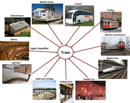
Figure 1: Context in the mind: What classes can trigger the idea of a “train”? Many classes have similar appearance but are semantically unrelated; others are semantically close but visually dissimilar. We argue that consistently co-firing classifiers, either based on spatial and temporal context or similar appearance, can be powerful in collaboration and robust to outliers, overfitting and missing features. Here, we show the classifiers that are consistently selected by our method, from very limited training data, as providing valuable input to the class “train”.

Feature selection is known to be NP-hard [16, 36], so finding the optimal solution to the combinatorial search is prohibitive. Thus, previous work has focused on greedy methods, such as sequential search [39] and boosting [15] or heuristic approaches, such as genetic algorithms [44]. We approach feature selection from a different direction, that of discriminant linear classification [10], with a novel constraint on the solution and the features. We put an upper bound on the solution weights and further require it to be an affine combination of soft-categorical features, which have to be also positively correlated with the positive class. Our constraints lead to a convex formulation with some important theoretical guarantees that strongly favor sparse optimal solutions with equal non-zero weights. This automatically becomes a feature selection mechanism, such that most features with zero weights can be ignored while the remaining few are averaged to become a strong group of classifiers with a single united voice.

Consider Fig. 1: here we use image-level CNN classifiers [21], pre-trained on ImageNet, to recognize trains in video frames from YouTube-Objects dataset [38]. Our method builds an ensemble from a pool of $6000$ classifiers ($1000$ ImageNet classifiers $\times$ $6$ image regions) that are potentially relevant to the concept. Since each classifier corresponds to one ImageNet concept, we directly visualize some of the classifiers (shown as sample images from corresponding classes) that are consistently selected by our method over $30$ trials on different small sets of $8$ video shots, each with just $10$ evenly spaced frames. We observe that the classes chosen may seem semantically different from train (e.g. library, greenhouse, steel bridge), but they are definitely related to the concept, either through appearance (e.g. library, greenhouse), through context (steel bridge), or both (sliding door).

2 Scientific Context

Decades of research in machine learning show that an ensemble can be significantly stronger than an individual classifier in isolation [9, 17], especially when the individual classifiers are diverse and make mistakes on different regions of the input space. There are many methods for ensemble learning that have been studied over the years [34, 9], with three main approaches: bagging [3], boosting [15] and decision trees ensembles [24, 6].

Bagging blindly samples from the training set to learn a different classifier for each sampled set, then takes the average response over all classifiers as the final answer. While this approach avoids overfitting, it does not explore deeper structure in the data and, in practice, the same classifier type is used for each random training subset. Different from bagging we select small subsets of relevant features over the whole training set. Our feature pool contains diverse and potentially strong classifiers (Fig. 3), either created from scratch or reused from pre-trained libraries (Sec. 5).

Boosting is a popular technique that in general outperforms bagging, as it searches for relevant features from a vast pool of candidates. It adds features one by one, in an efficient greedy fashion, to reduce the expected exponential loss. The sequential addition of features puts much more weight on the initial ones selected. If too much weight is given to the first features (when they are strong classifiers by themselves), boosting is less expected to form powerful classifier ensembles that help each other as a group, as the initial features selected will dominate. Thus, boosting works best with weak features, and has difficulty with more powerful ones, such as SVMs [31]. Our method is well suited for combining strong classifiers, which together form an even stronger group. They are discovered as clusters of co-firing classifiers that are independent given the class, but united on separating the positive class versus the rest. The balanced collaboration between classifiers encourages similar weights for each input feature. In turn, equal averaging leads to classifier independence given the class (Sec. 4).

Our method is also related to averaging decision trees. One of the main differences is that we do not average all of the classifiers: we identify the few most important ones and average over them. Averaging over a judicious set rather than blind averaging over the pool makes a significant difference (Fig. 2a). There is also work [43] on combining decision forests with ideas from boosting, in order to obtain a weighted average of trees that better fits the training data. Rather than consuming a significant amount of training data to fit optimal weights, our method focuses on finding subsets of features that will work well with known similar weights. By averaging strong subsets of diverse classifiers we obtain excellent accuracy and generalization, even from limited training data.

We are not the first to see a connection between clustering and feature selection. Some consider the inverse task: feature selection for unsupervised clustering [48, 25]. Others propose efficient selection of features through diversity [45]. However, we are the first to formulate supervised learning as an equivalent unsupervised clustering task.

In Section 5, we describe in more detail how we create novel powerful features by naturally clustering the training data over neighborhoods in descriptor space (CIFAR features), contiguous temporal regions in time (Youtube-Parts features) and spatial neighborhoods over different image windows/regions of presence (Youtube-Parts and ImageNet features). They provide intermediate lower level classifiers for the higher level problem of category understanding, in the presence of significant variations in scale, poses and viewpoints, intr-class variations, and large background clutter. These intermediate features could be seen as as building blocks in a hierarchical and potentially recursive recognition system, validating some of the ideas in [30].

The connection to hierarchical approaches based on Deep Nets [19, 18] is interesting, both from a feature creation and re-usability perspective, as well as from the viewpoint of building multi-layered hierarchical classifiers. The relation to other hierarchical approaches is also beneficial, given the many successful hierarchical approaches in computer vision, from the classifier cascades used for face detection [46], the Part-Based Model and Latent SVMs [12] applied to general object category detection, Conditional Random Fields [40], classification trees and random forests, probabilistic Bayesian networks, directed acyclic graphs (DAGs) [20], hierarchical hidden Markov models (HHMMs) [13] and methods using feature matching with second-order or hierarchical spatial constraints [27, 5, 26].

Main Contributions:

The contributions of our novel approach to learning discriminative sparse classifier averages are summarized below:

1. A novel approach to linear classification that is equivalent to unsupervised learning defined as a convex quadratic program, with efficient optimization. The global solution is sparse with equal weights effectively leading to a feature selection procedure. This is important since feature selection is known to be NP-hard.

2. An efficient clustering method that is one to two orders of magnitude faster in practice than interior point convex optimization, based on recent work on the IPFP algorithm [28] and the Frank-Wolfe method [14].

3. Compared to more sophisticated methods, such as AdaBoost and SVM, our algorithm exhibits better generalization with more modest computational and storage costs. Our training time is quadratic in the number of available features but constant in the number of training samples.

4. Efficient ways of automatically constructing powerful intermediate features as classifiers learned from various datasets (Section 5). This transfers knowledge from different image classification tasks to a new problem of recognition in video and provides the ability to re-use resources by transforming previously learned classifiers into input features to novel learning tasks. While learning auto-encoders [19, 41]) also effectively uses anonymous classifiers as input features to higher level interpretation layers, we provide a way to use apparently unrelated classifiers, learned from different data, as black boxes. Our linear discriminant approach to feature selection becomes an effective procedure of learning one layer at a time and further validates some of our proposals in [30]

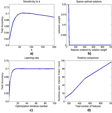
Figure 2: Optimization and sensitivity analysis: a) Sensitivity to $k$. Performance improves as features are added, is stable around the peak $k=60$ and falls $k>100$ as useful features are exhausted. b) Features ordered by weight for $k=50$ confirming that our method selects nearly equal weights up to the chosen $k$. c) Our method converges to a solution in $10$–$20$ iterations. d) Runtime of interior point method divided by ours, both in Matlab and with $100$ max iterations. All results are averages over $100$ random experiments.

3 Problem Formulation

We address the classical case of binary classification, with the one vs. all strategy being applied to the multi-class scenario as well. Given a set of $N$ training samples, with each $i$-th sample expressed as a vector $\mathbf{f}_{i}$ of $n$ possible features with values between $0$ and $1$, we want to find the weight vector $\mathbf{w}$, with non-negative elements and L1-norm $1$, such that $\mathbf{w}^{T}\mathbf{f}_{i}\approx p_{1}$ when the $i$-th sample is from class $1$ and $\mathbf{w}^{T}\mathbf{f}_{i}\approx p_{0}$ otherwise. As $p_{0}$ and $p_{1}$ represent the expected feature average output for negative and positive samples, respectively, then $0\leq p_{0}\leq p_{1}\leq 1$. We require the input features $\mathbf{f}_{i}$ to be positively correlated with class $1$; when they are not we simply flip their output, by setting $f_{i}(j)\leftarrow 1-f_{i}(j)$. Traditionally, $p_{0}=0$ and $p_{1}=1$, but we used $p_{0}=0$ and $p_{1}=0.5$, with slightly improved performance, as averages over positives are expected to be less than $1$.

In order to limit the impact of each individual feature we restrict the elements of $\mathbf{w}$ to be between $0$ and $1/k$, and sum up to $1$. Our formulation is similar to linear classification with the added constraints that the input features themselves could represent other classifiers and the linear separator $\mathbf{w}$ acts as an affine combination of their outputs, to produce a weighted feature average $\mathbf{w}^{T}\mathbf{f}_{i}\in[0,1]$. In Section 4 we show that the value of $k$ has a direct role on the sparsity of the solution and the number of features that have strong weights, a fact validated by our experiments.

Given the $N\times n$ feature data matrix $\mathbf{F}$ and ground truth vector $\mathbf{t}$, the learning problem becomes finding $\mathbf{w^{*}}$ that minimizes the sum of squares error $J(\mathbf{w})=\|\mathbf{Fw}-\mathbf{t}\|^{2}$, under the constraints on $\mathbf{w}$. We obtain the convex problem:

$$\mathbf{w^{*}} = \operatorname*{argmin}_{w}J(\mathbf{w})=\operatorname*{argmin}_{w}\|\mathbf{Fw}-\mathbf{t}\|^{2}$$

$$= \operatorname*{argmin}_{w}\mathbf{w^{\top}(F^{\top}F)w}-2\mathbf{(Ft)}^{\top}\mathbf{w}+\mathbf{t}^{\top}\mathbf{t}$$

$$s.t.\sum_{i}w_{i}=1\;,\;w_{i}\in[0,1/k].$$

Since $\mathbf{t}$ is the ground truth, the last term is constant. After dropping it, we note that the supervised learning task is a special case of clustering with pairwise and unary terms, as defined in  [4, 32, 29]. Note that our formulation can be easily changed into a concave maximization problem by changing the signs of the terms. Since the algorithm of [29] works with both positive and negative terms, we adapt their efficient optimization scheme that achieves near-optimal solutions in only $10-20$ iterations.

The connection to clustering is interesting and makes sense. Feature selection can be interpreted as a clustering problem: we seek a group of features that are individually relevant, but not redundant with respect to each other — an observation consistent with earlier research in machine learning (e.g., [9]) and neuroscience (e.g., [42]). This idea is also related to the recent work on discovering discriminative groups of HOG filters [1], but different from that and other previous work, in that ours transforms the supervised learning task into an equivalent unsupervised clustering problem. To get a better intuition let us examine in more detail the two terms of the objective, the quadratic one $\mathbf{w^{\top}(F^{\top}F)w}$ and the linear term $-2\mathbf{(Ft)}^{\top}\mathbf{w}$. If we assume that feature outputs have similar means and standard deviations over training samples (a fact that could be obtained by appropriate normalization), then minimizing the linear term boils down to giving more weight to features that are more strongly correlated with the ground truth. This is expected, since they are the ones that are best for classification by themselves. On the other hand, the matrix $\mathbf{F^{\top}F}$ contains the dot-products between pairs of feature responses over the training set. Then, minimizing $\mathbf{w^{\top}(F^{\top}F)w}$ should find groups of features that are as uncorrelated as possible. The value of $1/k$ limits the weight put on any single input classifier and requires the final solution to have nonzero weights for at least $k$ features. In Section 4 we present analysis that the solution preferred is sparse, very often having exactly $k$ features with uniform weights of value exactly $1/k$.

4 Theoretical Analysis

The optimization problem is convex and can be globally solved in polynomial time. We adapted the integer projected fixed point method from [29] to the case of unary and pairwise terms, which is very efficient in practice (Fig. 2c). The optimization procedure is iterative and approximates at each step the original error function with a linear, first-order Taylor approximation that can be solved immediately. That step is followed by a line search with rapid closed-form solution, and the process is repeated until convergence. Please see [29, 28] for more details. In practice, after only $10$–$20$ iterations we are very close to the optimum, but we used $100$ iterations in all our experiments. The theoretical guarantees at the optimum prove that Problem 3 prefers sparse solution with equal weights, also confirmed in practice (Fig. 2b).

Proposition 1: Let $\mathbf{d(w)}=2\mathbf{F^{\top}Fw-F^{\top}t}$ be the gradient of $J(\mathbf{w})$. The partial derivatives $d(\mathbf{w})_{i}$ corresponding to those elements $w^{*}_{i}$ of the global optimum of Problem 3 with non-sparse, real values in $(0,1/k)$ must be equal to each other.

Proof: The global optimum of Problem 3 satisfies the Karush-Kuhn-Tucker (KKT) necessary optimality conditions. The Lagrangian function of (3) is:

$$L(\mathbf{w},\lambda,\mu,\beta) = J(\mathbf{w})-\lambda(\sum w_{i}-1)+$$ (2)

$$\sum\mu_{i}w_{i}+\sum\beta_{i}(1/k-w_{i}),$$

From the KKT conditions at a point $\mathbf{w^{*}}$ we have:

$$\begin{array}[]{l}\mathbf{d(w^{*})}-\lambda+\mu_{i}-\beta_{i}=0,\\ \sum_{i=1}^{n}\mu_{i}w^{*}_{i}=0,\\ \sum_{i=1}^{n}\beta_{i}(1/k-w^{*}_{i})=0.\\ \end{array}$$

Here $\mathbf{w^{*}}$ and the Lagrange multipliers have non-negative elements, so if $w_{i}>0\Rightarrow\mu_{i}=0$ and $w_{i}<1/k\Rightarrow\beta_{i}=0$. Then there must exist a constant $\lambda$ such that we have:

$$d(\mathbf{w^{*}})=\left\{\begin{array}[]{ll}\leq\lambda,&w^{*}_{i}=0,\\ =\lambda,&w^{*}_{i}\in(0,1/k),\\ \geq\lambda,&w^{*}_{i}=1/k.\\ \end{array}\right.$$

This implies that all partial derivatives of $d(\mathbf{w^{*}})$ that are not in $[0,1/k]$ must be equal to some constant $\lambda$, therefore they must be equal to each other, which concludes our proof.

From Proposition $1$ it follows that in the general case, when the partial derivatives at the optimum point are unique, the elements of the optimal $\mathbf{w^{*}}$ are either $0$ or $1/k$. Since the sum over the elements of $\mathbf{w^{*}}$ is $1$, it is further implied that the number of nonzero elements in $\mathbf{w^{*}}$ is often $k$. Thus, our solution is not just a simple linear separator (hyperplane), but also a sparse representation and a feature selection procedure that effectively averages the selected $k$ or close to $k$ features. To enable a better statistical interpretation of these sparse averages, we consider the somewhat idealized case when all features have equal means $(p_{1},p_{0})$ and equal standard deviations $(\sigma_{1},\sigma_{0})$ over the positive and negative training sets, respectively.

Proposition 2: If we assume that the input soft classifiers are independent and better than random chance, the error rate converges towards $0$ as their number $n$ goes to infinity.

Proof: Given a classification threshold $\theta$ for $\mathbf{w}^{T}\mathbf{f}_{i}$, such that $p_{0}<\theta<p_{1}$, then, as $n$ goes to infinity, the probability that a negative sample will have an average response greater than $\theta$ (a false positive mistake) goes to $0$. This follows from Chebyshev’s inequality (or the Law of Large Numbers). By a similar argument, the probability of a false negative also goes to zero as $n$ goes to infinity.

Proposition 3: The weighted average $\mathbf{w}^{T}\mathbf{f}_{i}$ with smallest variance over positives (and negatives, respectively) has equal weights.

Proof: We consider the case when $\mathbf{f}_{i}$’s are features of positive samples, the same argument being true for the negative ones. We have: $\text{Var}(\sum_{i}w_{i}f_{i}/\sum_{i}w_{i})=\sum w_{i}^{2}/(\sum w_{i})^{2}\sigma^{2}_{1}$. We find the minimum of $\sum w_{i}^{2}/(\sum w_{i})^{2}$ by setting its partial derivatives to zero and obtain $w_{j}(\sum w_{i})=\sum w_{i}^{2},\forall j$. Therefore, $w_{i}=w_{j},\forall i,j$.

Equal weights minimize the output variances over positives, and over negatives, separately (P3), so they are most likely to minimize the error rate, when the features are independent and follow the equal means and variance assumptions above (P2). This is important, since our method will certainly find the set of features with equal weights (in general) that minimize the convex error objective 3 (P1).

Computational aspects:

Compared to the general case of arbitrary real weights for all possible features, the averaging solution preferred by Problem 3 requires considerably less memory. The average of $k$ selected features out of $N$ possible requires about $k\log_{2}N$ bits, whereas having a real weight for each possible feature requires $32N$ bits in floating point representation. Sparse solutions are simpler in terms of representation but have good accuracy and considerably smaller computational cost (Fig. 4) than the more costly SVM and AdaBoost. They seem to follow closer the Occam’s Razor principle [2], which would explain in part their good performance and generalization. The computational cost of the optimization method we use is $O(Sn^{2})$ [29], where $S$ is the number of iterations and $n$ is the number of features. In our experiments we use $S=100$, even though $S=20$ would suffice. The more general interior point method for convex optimization using Matlab’s $quadprog$ is polynomial, but considerably slower than ours, by a factor that increases linearly with features pool size (see Fig. 2). For $125$ features it is $9$ times slower, and for $1000$ features, about $100$ times slower.

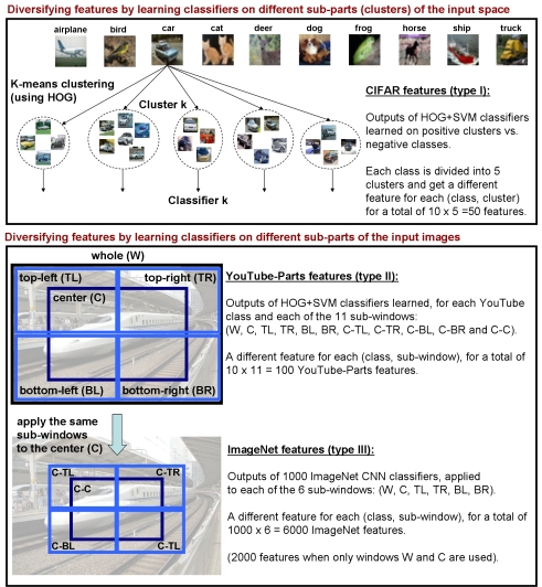
Figure 3: We encourage feature diversity and independence by taking classifiers trained on 3 datasets (CIFAR, YouTube-Objects and ImageNet) and by looking at different parts of the input space (Type I) or different locations within the image (Types II and III). Experiments confirm the benefits of diversity.

5 Learning the Feature Pool

We created a large pool of over $6000$ different features, computed and learned from three different datasets: CIFAR [23], ImageNet [8] and a hold-out part of the YouTube-Objects training set. More details about creating our features follow next and are also summarized in Fig. 3.

CIFAR features (type I):

This dataset contains $60000$ 32$\times$32 color images in $10$ classes (airplane, automobile, bird, cat, deer, dog, frog, horse, ship, truck), with $6000$ images per class. There are 50000 training images and 10000 test images. We randomly chose $2500$ images per class for creating our features. They are HOG+SVM classifiers trained on data obtained by clustering images from each class into $5$ groups using k-means applied to their HOG descriptors. Each classifier had to separate its own cluster versus images from other classes. We hoped to obtain, for each class, diverse and relatively independent classifiers, which respond to different parts of the input space that are naturally clustered. Note that CIFAR categories coincide only partially ($7$ out of $10$ with the ones from YouTube-Objects). The output of each of the $5\times 10=50$ such classifiers becomes a different input feature, which we compute on all training and test images from YouTube-Objects.

YouTube-parts features (type II):

We formed a separate dataset with $25000$ images from video, randomly selected from a subset of YouTube-Objects Training videos, not used in subsequent learning and recognition experiments. Features are outputs of linear SVM classifiers using HOG applied to the different parts of each image. Each classifier is trained and applied to its own dedicated sub-window as shown in Fig. 3. To speed up training and remove noise we also applied PCA to the resulted HOG, and obtained descriptors of $46$ dimensions, before passing them to SVM. For each of the $10$ classes, we have $11$ classifiers, one for each sub-window, and get a total of $110$ type II features. Experiments with a variety of SVM kernels and settings showed that linear SVM with default parameters for libsvm worked best, and we kept that fixed in all experiments.

ImageNet features (type III):

We considered the soft feature outputs (before soft max) of the pre-trained ImageNet CNN features using Caffe [21], each of them over six different sub-windows: whole, center, top-left, top-right, bottom-left, bottom-right, as presented in Fig. 3. There are $1000$ such outputs, one for each ImageNet category, for each sub-window, for a total of $6000$ features. In some of our experiments, when specified, we used only $2000$ ImageNet features, restricted to the whole and center windows.

6 Experimental Analysis

We evaluate our method’s ability to generalize and learn quickly from limited data as well as transfer and combine knowledge from different datasets, containing video or low- and medium-resolution images of many potentially unrelated classes. We evaluate its performance in the context of recognition in video and report recognition accuracy per frame. We compare to established methods and analyze the behavior of all algorithms along different experimental dimensions, by varying the kinds and number of potential input features used, number of shots chosen for training as well as the number of frames selected per shot. We pay particular attention, besides the test accuracy, to train vs. test accuracy (over-fitting) and training time. We choose the large-scale YouTube-Objects video dataset [38], with difficult sequences of ten categories (aeroplane, bird, boat, car, cat, cow, dog, horse, motorbike, train) taken in the wild. The training set contains about $4200$ video shots, for a total of $436970$ frames, while the test set has $1284$ video shots for a total of over $134119$ frames. The videos display significant background clutter, with objects coming in and out of foreground focus, undergoing occlusions and significant changes in scale and viewpoint. More importantly, the intra-class variation is large and sudden between video shots. Given the very large number of frames and variety of shots, their complex appearance and variation in length, presence of background clutter and many other objects, changes in scale, viewpoint and drastic intra-class variation, the task of recognizing the main category from only a few frames becomes a real challenge. We used the same training/testing split as in [38]. In all our tests, we present results averaged over $30-100$ random experiments, for all methods compared.

Table 1: Distribution in percentages of sub-windows (Fig. 3) for selected ImageNet classifiers per category. Note that different categories that seem superficially similar (e.g., cats and dogs) generate very different distributions (see text).

Locations	W	C	TL	TR	BL	BR
aeroplane	65.6	30.2	0	0	2.1	2.1
bird	78.1	21.9	0	0	0	0
boat	45.8	21.6	0	0	12.3	20.2
car	54.1	40.2	2.0	0	3.7	0
cat	76.4	17.3	5.0	0	1.3	0
cow	70.8	22.2	1.8	2.4	0	2.8
dog	92.8	6.2	1.0	0	0	0
horse	75.9	14.7	0	0	8.3	1.2
motorbike	65.3	33.7	0	0	0	1.0
train	56.5	20.0	0	2.4	12.8	8.4

We evaluated six methods: ours, SVM on all input features, AdaBoost on all input features, ours with SVM (applying SVM only to features selected by our method, idea related to [37, 47, 22]), forward-backward selection (FoBa) [50] and simple averaging over all input features. Recognition rate is computed per frame. Input features have soft-values between $0$ and $1$ and are expected to be positively correlated with the positive class (we remember during training which feature should be flipped for which class). For our method, which outputs a sparse solution as a weighted average over a few features, we select those with a weight larger than a very small threshold. Note that once features are selected, in principle, any classifier could be learned, to fine-tune the weights, as is the case with ours with SVM. While FoBa works directly with the features given, AdaBoost further transforms each feature into a weak hard classifier by choosing the threshold that minimizes the expected exponential loss, at each iteration; that is one reason why AdaBoost is much slower w.r.t. to the others.

Table 1 summarizes the locations distribution of ImageNet features selected by our method for each category in YouTube-Objects. We make several observations. First, the majority of features for all classes consider the whole image (W), which suggests that the image background is relevant. Second, for several categories (e.g., car, motorbike, aeroplane), the center (C) is important. Third, some categories (e.g., boat) may be located off-center or benefit from classifiers that focus on non-central regions. Finally, we see that object categories that may superficially seem similar (cat vs. dog) exhibit rather different distributions: dogs seem to benefit from the whole image while cats benefit from sub-windows; this may be because cats are smaller and appear in more diverse contexts and locations, particularly in YouTube videos. We evaluated the performance of all methods by varying the number of shots randomly chosen for training and averaged the results over $30-100$ experiments.

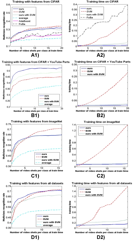
Figure 4: Accuracy and training time on YouTube-Objects, with varying training video shots ($10$ frames per shot and results averaged over $30$ runs). Input feature pool, row 1: $50$ type I features on CIFAR; row 2: $110$ type II features on YouTube-Parts + $50$ CIFAR; row 3: $2000$ type III features in ImageNet; row 4: $2160$ all features. Ours outperforms SVM, AdaBoost and FoBa (see text).

The results, presented in Fig. 4, show convincingly that our method has a constant training time, and is much less costly than SVM, AdaBoost (time too large to show in the plot) and FoBa. Moreover, our method is able to outperform significantly most methods (even SVM in many cases). As our intuition and theoretical results suggested, the proposed discriminative feature clustering approach is superior to the others as the amount of training data is more limited (also see Figs. 5 and 6). Our mining of powerful groups of classifiers from a vast sea of candidates from limited data is a novel direction, complementary to learning approaches that spend significant training time and data to fit optimal real weights over many features. We also validate the importance of the feature pool size and quality (Table 2).

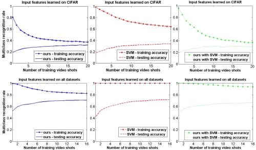
Figure 5: Our method generalizes (training and test errors are closer) compared to SVM or in combination with SVM.

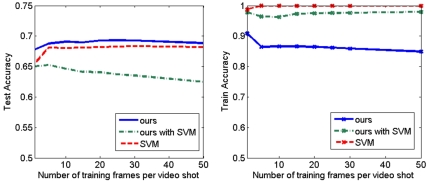
Figure 6: Average test recognition accuracy over $30$ independent experiments of our method as we vary the number of training frames uniformly sampled from random $8$ training video shots. Note how well our method generalizes from as few as $1$ frame per video shot, for a total of $8$ positive training frames per class.

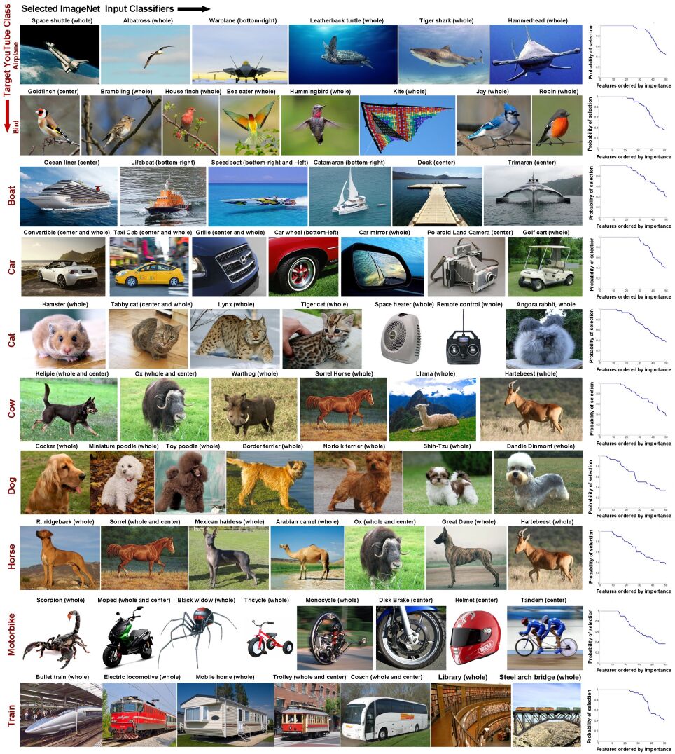
Figure 7: For each training target class from YouTube-Objects videos (labels on the left), we present the most frequently selected ImageNet classifiers (input features), over $30$ independent experiments, with $10$ frames per shot and $10$ random shots for training. In images we show the classes that were always selected by our method when $k=50$. On the right we show the probability of selection for the most important $50$ features. Note how stable the selection process is. Also note the interesting connections between the selected classes and the target class in terms of appearance, context or geometric part-whole relationships. We find two aspects indeed interesting: 1) the high probability (perfect 1) of selection of the same classes, even for such small random training sets and 2) the fact that unrelated classes in terms of meaning could be so useful for classification, based on their shape and appearance similarity.

Table 2: Accuracy on YouTube-Objects with varying number of training shots for different feature pools. Accuracy doubles with the size and diversity of the pool.

Accuracy	I ($50$)	I+II ($160$)	I+II+III ($6160$)
$10$ train shots	29.69%	51.57%	69.99 %
$20$ train shots	31.97%	52.37%	71.31 %

Intuition and qualitative results:

An interesting finding in our experiments (see Fig. 7) is the consistent discovery, for a given target class, of selected input classifiers that are related to the main one in surprising ways: 1) similar w.r.t. global visual appearance, but not semantic meaning – banister vs. train, tigershark vs. plane, Polaroid camera vs. car, scorpion vs. motorbike, remote control vs. cat’s face, space heater vs. cat’s head; 2) related in co-occurrence and context, but not in global appearance – helmet vs. motorbike; 3) connected through part-to-whole relationships – grille, mirror and wheel vs. car; or combinations of the above – dock vs. boat, steel bridge vs. train, albatross vs. plane. The relationships between the target class and the input, supporting classes, could also hide combinations of many other factors. Meaningful conceptual relationships could ultimately join together correlations along many dimensions, from appearance to geometric, temporal and interaction-like relations.

Another interesting aspect is that the classes found are not necessarily central to the main category, but often peripheral, acting as guardians that separate the main class from the rest. This is where feature diversity plays an important role, ensuring both separation from nearby classes as well as robustness to missing values.

An additional possible benefit is the capacity to immediately learn novel concepts from old ones, by combining existing high-level concepts to recognize new classes. In cases where there is insufficient data for a particular new class, sparse averages of reliable classifiers can be an excellent way to combine previous knowledge. Consider the class cow in Fig. 7. Although “cow” is not present in the $1000$ label set, our method is able to learn the concept by combining existing classifiers.

Since categories share shapes, parts and designs, it is perhaps unsurprising that classifiers trained on semantically distant classes that are visually similar can help improve learning and generalization from limited data.

7 Conclusions

We have presented an efficient method for joint selection of discriminative and diverse groups of features that are independent by themselves and strong in combination. Our feature selection solution comes directly from a supervised linear classification problem with specific affine and size constraints, which can be solved rapidly due to its convexity. Our approach is able to quickly learn from limited data effective classifiers that outperform in time and even accuracy more established methods such as SVM, Adaboost and greedy sequential selection. We also propose different ways of creating novel, diverse features, by learning separate classifiers over the input space and over different regions in the input image. Having a training time that is independent of the number of input images and an effective way of learning from large and heterogeneous feature pools, our approach provides a useful tool for many recognition tasks, suited for real-time, dynamic environments. Based on our extensive experiments we believe that it has the potential to strengthen the connection between the apparently separate problems of unsupervised clustering, linear discriminant analysis and feature selection.

Acknowledgments:

This work was supported by CNCS-UEFICSDI, under project PNII PCE-2012-4-0581. The authors would like to thank Shumeet Baluja for interesting discussions and helpful feedback.

References

- [1] E. Ahmed, G. Shakhnarovich, and S. Maji. Knowing a good HOG filter when you see it: Efficient selection of filters for detection. In ECCV, 2014.
- [2] A. Blumer, A. Ehrenfeucht, D. Haussler, and M. Warmuth. Occam’s razor. Information processing letters, 24(6), 1987.
- [3] L. Breiman. Bagging predictors. Machine learning, 24(2), 1996.
- [4] S. Bulo and M. Pellilo. A game-theoretic approach to hypergraph clustering. In NIPS, 2009.
- [5] D. Conte, P. Foggia, C. Sansone, and M. Vento. Thirty years of graph matching in pattern recognition. IJPRAI, 18(3), 2004.
- [6] A. Criminisi, J. Shotton, and E. Konukoglu. Decision forests: A unified framework for classification, regression, density estimation, manifold learning and semi-supervised learning. Foundations and Trends® in Computer Graphics and Vision, 7(2–3), 2012.
- [7] N. Cuntoor and R. Chellappa. Key frame-based activity representation using antieigenvalues. In ACCV, 2006.
- [8] J. Deng, W. Dong, R. Socher, L. Li, K. Li, and L. Fei-Fei. ImageNet: A large-scale hierarchical image database. In CVPR, 2009.
- [9] T. Dietterich. Ensemble methods in machine learning. Springer, 2000.
- [10] R. Duda and P. Hart. Pattern classification and scene analysis. Wiley, 1973.
- [11] C. Ellis, S. Masood, M. Tappen, J. L. Jr., and R. Sukthankar. Exploring the trade-off between accuracy and observational latency in action recognition. IJCV, August 2012.
- [12] P. Felzenszwalb, R. Girshick, D. McAllester, and D. Ramanan. Object detection with discriminatively trained part-based models. PAMI, 32(9), 2010.
- [13] S. Fine, Y. Singer, and N. Tishby. The hierarchical hidden Markov model: Analysis and applications. Machine Learning, 32(1), 1998.
- [14] M. Frank and P. Wolfe. An algorithm for quadratic programming. Naval Research Logistics Quarterly, 3(1-2):95–110, 1956.
- [15] Y. Freund and R. Schapire. A decision-theoretic generalization of on-line learning and an application to boosting. In Comp. learn. theory, 1995.
- [16] I. Guyon and A. Elisseeff. An introduction to variable and feature selection. The Journal of Machine Learning Research, 3:1157–1182, 2003.
- [17] L. Hansen and P. Salamon. Neural network ensembles. PAMI, 12(10), 1990.
- [18] G. Hinton. A practical guide to training restricted Boltzmann machines. Momentum, 9(1), 2010.
- [19] G. Hinton, S. Osindero, and T. Yee-Whye. A fast learning algorithm for deep belief nets. Neural Computation, 18(7), 2006.
- [20] F. V. Jensen and T. D. Nielsen. Bayesian networks and decision graphs. Springer, 2007.
- [21] Y. Jia, E. Shelhamer, J. Donahue, S. Karayev, J. Long, R. Girshick, S. Guadarrama, and T. Darrell. Caffe: Convolutional architecture for fast feature embedding. In ACM Multimedia, 2014.
- [22] K. Kira and L. Rendell. The feature selection problem: Traditional methods and a new algorithm. In AAAI, 1992.
- [23] A. Krizhevsky and G. Hinton. Learning multiple layers of features from tiny images. Comp. Sci. Dep, Univ. of Toronto, Tech. Rep, 2009.
- [24] S. Kwok and C. Carter. Multiple decision trees. Uncertainty in Artificial Intelligence, 1990.
- [25] M. H. Law, M. A. Figueiredo, and A. Jain. Simultaneous feature selection and clustering using mixture models. PAMI, 26(9), 2004.
- [26] S. Lazebnik, C. Schmid, and J. Ponce. Beyond bags of features: Spatial pyramid matching for recognizing natural scene categories. In CVPR, 2006.
- [27] M. Leordeanu, M. Hebert, and R. Sukthankar. Beyond local appearance: Category recognition from pairwise interactions of simple features. In CVPR, 2007.
- [28] M. Leordeanu, M. Hebert, and R. Sukthankar. An integer projected fixed point method for graph matching and map inference. In NIPS, 2009.
- [29] M. Leordeanu and C. Sminchisescu. Efficient hypergraph clustering. In International Conference on Artificial Intelligence and Statistics, 2012.
- [30] M. Leordeanu and R. Sukthankar. Thoughts on a recursive classifier graph: a multiclass network for deep object recognition. arXiv preprint arXiv:1404.2903, 2014.
- [31] X. Li, L. Wang, and E. Sung. AdaBoost with SVM-based component classifiers. Engineering Applications of Artificial Intelligence, 21(5), 2008.
- [32] H. Liu, L. Latecki, and S. Yan. Robust clustering as ensembles of affinity relations. In NIPS, 2010.
- [33] D. Lowe. Distinctive image features from scale-invariant keypoints. IJCV, 60(4), 2004.
- [34] R. Maclin and D. Opitz. Popular ensemble methods: An empirical study. arXiv:1106.0257, 2011.
- [35] J. Mutch and D. Lowe. Multiclass object recognition with sparse, localized features. In CVPR, 2006.
- [36] A. Ng. On feature selection: learning with exponentially many irrelevant features as training examples. In ICML, 1998.
- [37] M. Nguyen and F. De la Torre. Optimal feature selection for support vector machines. Pattern recognition, 43(3), 2010.
- [38] A. Prest, C. Leistner, J. Civera, C. Schmid, and V. Ferrari. Learning object class detectors from weakly annotated video. In CVPR, 2012.
- [39] P. Pudil, J. Novovičová, and J. Kittler. Floating search methods in feature selection. Pattern recognition letters, 15(11), 1994.
- [40] A. Quattoni, S. Wang, L. Morency, M. Collins, and T. Darrell. Hidden conditional random fields. PAMI, 10(29), 2007.
- [41] S. Rifai, P. Vincent, X. Muller, X. Glorot, and Y. Bengio. Contractive auto-encoders: Explicit invariance during feature extraction. In International Conference on Machine Learning, pages 833–840, 2011.
- [42] E. Rolls and G. Deco. The noisy brain: stochastic dynamics as a principle of brain function, volume 34. Oxford university press Oxford, 2010.
- [43] S. Schulter, P. Wohlhart, C. Leistner, A. Saffari, P. Roth, and H. Bischof. Alternating decision forests. In CVPR, pages 508–515, 2013.
- [44] W. Siedlecki and J. Sklansky. A note on genetic algorithms for large-scale feature selection. Pattern recognition letters, 10(5), 1989.
- [45] N. Vasconcelos. Feature selection by maximum marginal diversity: optimality and implications for visual recognition. In CVPR, 2003.
- [46] P. Viola and M. Jones. Robust real-time face detection. IJCV, 57(2), 2004.
- [47] J. Weston, S. Mukherjee, O. Chapelle, M. Pontil, T. Poggio, and V. Vapnik. Feature selection for svms. In NIPS, volume 12, 2000.
- [48] Y. Yang, H. T. Shen, Z. Ma, Z. Huang, and X. Zhou. L2, 1-norm regularized discriminative feature selection for unsupervised learning. In IJCAI, 2011.
- [49] M. Zanfir, M. Leordeanu, and C. Sminchisescu. The moving pose: An efficient 3d kinematics descriptor for low-latency action recognition and detection. In ICCV, 2013.
- [50] T. Zhang. Adaptive forward-backward greedy algorithm for sparse learning with linear models. In NIPS, 2009.