Universität Siegen, D-57068 Siegen, Germanybbinstitutetext: Faculty of Physics, University of Warsaw, PL-00-681 Warsaw, Poland
Four-body contributions to at NLO
Abstract
Ongoing efforts to reduce the perturbative uncertainty in the decay rate have resulted in a theory estimate to NNLO in QCD. However, a few contributions from multi-parton final states which are formally NLO are still unknown. These are parametrically small and included in the estimated error from higher order corrections, but must be computed if one is to claim complete knowledge of the rate to NLO. A major part of these unknown pieces are four-body contributions corresponding to the partonic process . We compute these NLO four-body contributions to , and confirm the corresponding tree-level leading-order results. While the NLO contributions arise from tree-level and one-loop Feynman diagrams, the four-body phase-space integrations make the computation non-trivial. The decay rate contains collinear logarithms arising from the mass regularization of collinear divergences. We perform an exhaustive numerical analysis, and find that these contributions are positive and amount to no more than of the total rate in the Standard Model, thus confirming previous estimates of the perturbative uncertainty.
Keywords:
Rare decays, NLO calculations, Standard Model1 Introduction
The inclusive radiative meson decay is the paradigm for precision tests of the Standard Model (SM) in quark flavor physics. Its branching ratio is measured with a precision of cleo ; belle ; babar ; HFAG 111 The semi-inclusive measurement in the first reference in belle has recently been superseded by a new, more precise one – see Ref. 1411.3773 . However, this new measurement is not yet taken into account in the HFAG average of Eq. (1). ,
| (1) |
To match this experimental precision, a theory calculation to next-to-next-to-leading order (NNLO) accuracy is necessary. This program has been carried out during the last two decades and it is almost – but not quite – finished. The current theory estimate results in the following value 0609232 :
| (2) |
where the total uncertainty is due to non-perturbative (5%), parametric (3%), higher orders (3%) and -interpolation ambiguity (3%) 0609232 .
The calculation can be divided into: 1. Matching conditions 9308349 ; 9703349 ; 9710336 ; 9710335 ; 9904413 ; 9910220 ; 0007259 ; 0109058 ; 0401041 , 2. Anomalous dimensions 9211304 ; 9304257 ; 9409454 ; 9612313 ; 9711280 ; 9711266 ; 0306079 ; 0411071 ; 0504194 ; 0612329 , and 3. Matrix elements 9506374 ; 9512252 ; 9602281 ; 9603404 ; 9903305 ; 0105160 ; 0203135 ; 0302051 ; 0505097 ; 0506055 ; 0605009 ; 0607316 ; 0609241 ; 0707.3090 ; 0805.3911 ; 1005.1173 ; 1005.5587 ; 1009.2144 ; 1009.5685 ; 1209.0965 . Matching conditions and anomalous dimensions are complete up to NNLO since a long time. Missing pieces include -dependent matrix elements at NNLO 0609241 ; HCMSinprep , as well as next-to-leading-order (NLO) matrix elements proportional to penguin or CKM-suppressed current-current operators. The latter are formally NLO but are suppressed by very small Wilson coefficients, and should indeed be rather small, fitting within the estimated uncertainty from higher orders 0104034 ; 0609232 . However, only a full calculation can provide precise knowledge of their true effect, and we intend to do that here. This work constitutes part of an ongoing effort to reduce the perturbative uncertainty down to a negligible level.
The rate is given by the inclusive partonic rate of the quark, up to non-perturbative effects that, for a photon energy cut GeV, are estimated at the level of 1003.5012 ,
| (3) |
where denotes the partonic decay of the quark into any number of particles with an overall strangeness , plus a hard photon with , and excluding charm:
| (4) |
with . Each individual rate is an interference of different amplitudes, computed as matrix elements of local operators in the effective Lagrangian:
| (5) |
where the operators are defined as 9612313 :
| (6) |
With this notation, contain CKM phases: , with and defined in the usual way, e.g. Ref. 9612313 . We will also use the notation etc. The other Wilson coefficients are simply as in Ref. 9612313 .
For more than two final state particles, the rate involves integration over phase space; the photon spectrum opens up, and the rate depends on the photon-energy cut. The perturbative contribution can be written, in the notation of Ref. 0506055 , as:
| (7) |
summed over , and with the normalization
| (8) |
The “effective” Wilson coefficients are , and . Throughout the paper we use the NDR- scheme with fully anti-commuting .
The objects arise from the interference of operators and in the squared matrix elements, integrated over phase space. They depend on the photon energy cut through the variable . In the notation of Ref. 0609241 , where normalization to the inclusive semileptonic rate is used, , with 9903226 .
In this paper we focus on the four-body contributions to , corresponding to :
| (9) |
where we define as the contribution to . In addition, we expand as:
| (10) |
There is a hierarchy in the size of the Wilson coefficients of the operators in Eq. (6), which can be divided into two classes:
| (11) |
Operators in class have large Wilson coefficients, whereas class- operators have either very small Wilson coefficients or are CKM-suppressed. Among the four-body leading and next-to leading contributions we distinguish four groups:
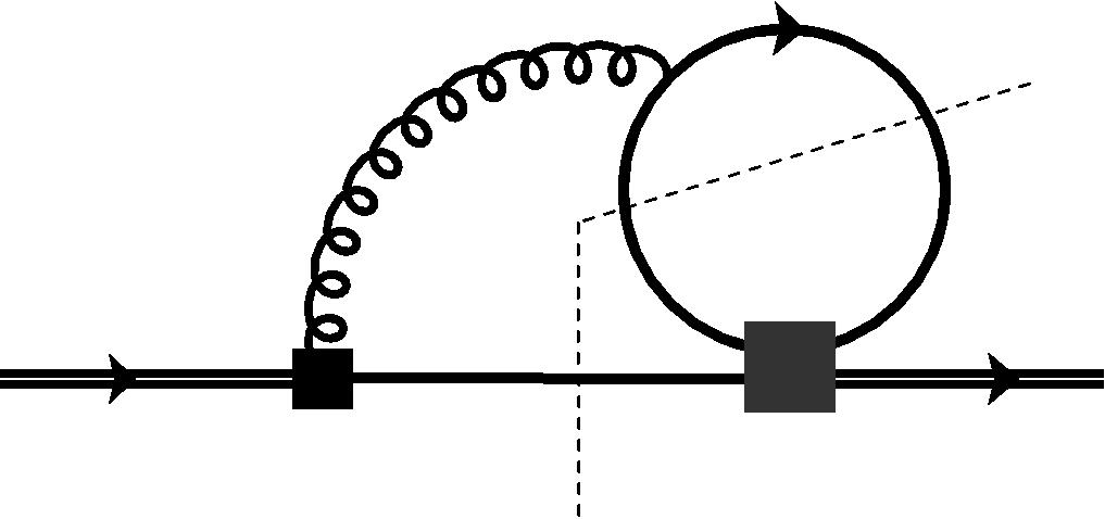
- •
- •
-
•
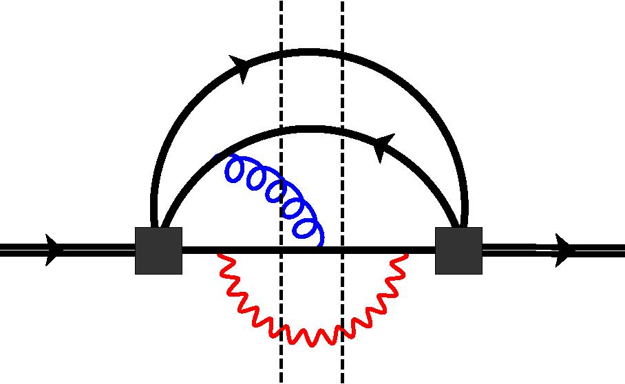
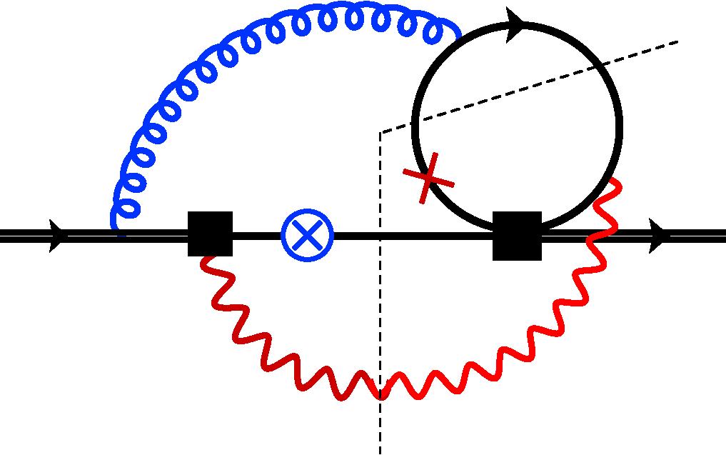
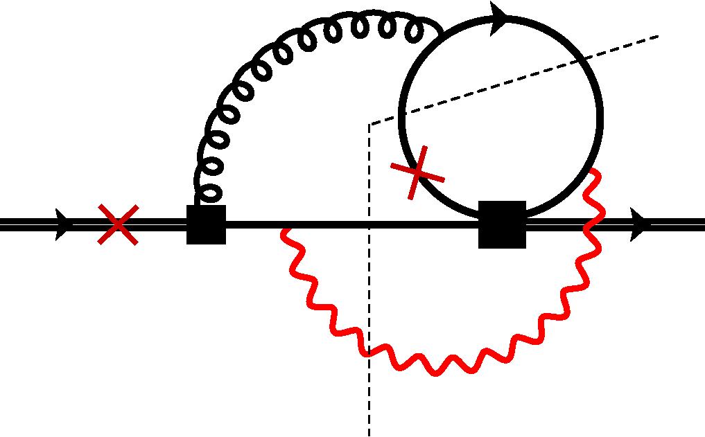
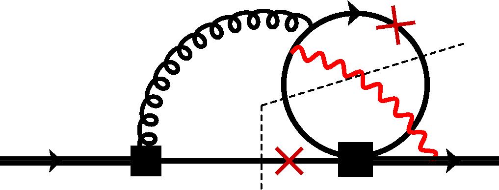
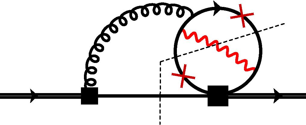
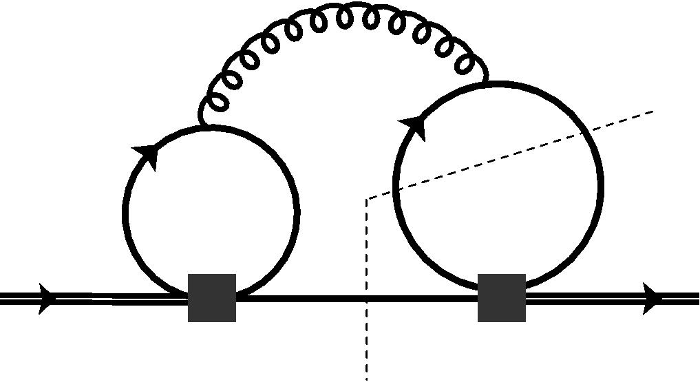
One-loop interference (Fig. 1.d). These are NLO and provide the matrix elements , with and .
-
•
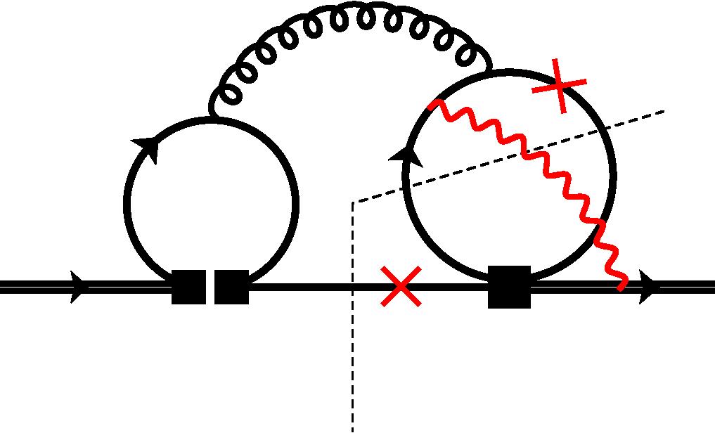
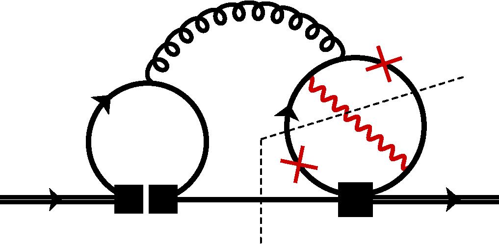
One-loop interference (Figs. 1.e and 1.f). The ones in panel (e) can be obtained from the ones in panel (d) as discussed in Section 2.1, and provide the matrix elements , with . The ones in panel (f) include five-particle cuts since the one-loop four-body diagrams must be complemented with the five-body gluon-bremsstrahlung correction . We therefore leave the contributions from panel (f) aside from the present four-body calculation.
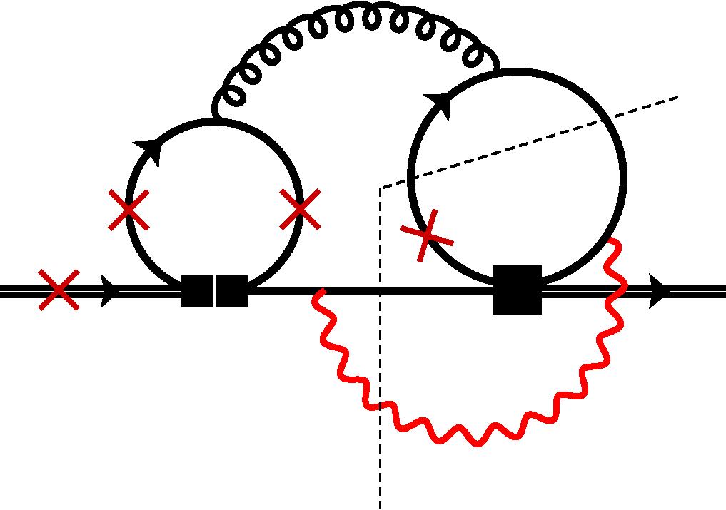
We note that NLO interference terms are presumably as large as the interference at the LO since . For the same reason, the partly neglected interference terms at the NLO are expected to be much smaller than the interferences that we calculate in a complete manner. As a final comment, we note that four-body NNLO contributions of the type are part of the calculation in Ref. HCMSinprep , and do not interfere with our results.
The structure of the paper is the following. In Section 2 we discuss the details of our calculation and the structure of the different contributions, including the set of diagrams needed, the UV renormalization, and the treatment of collinear divergences. In Section 3 we collect the final results. In Section 4 we perform a numerical study of all the evaluated interferences. Section 5 contains our conclusions. In Appendix A we collect some intermediate results of the calculation, where analytic cancellation of UV and collinear divergences can be explicitly checked.
2 Details of the calculation
The NLO calculation is performed in 4 steps:
-
1.
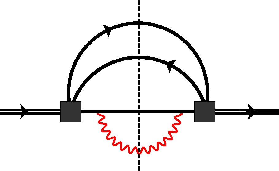
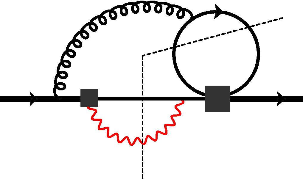
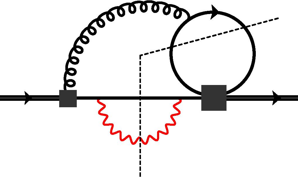
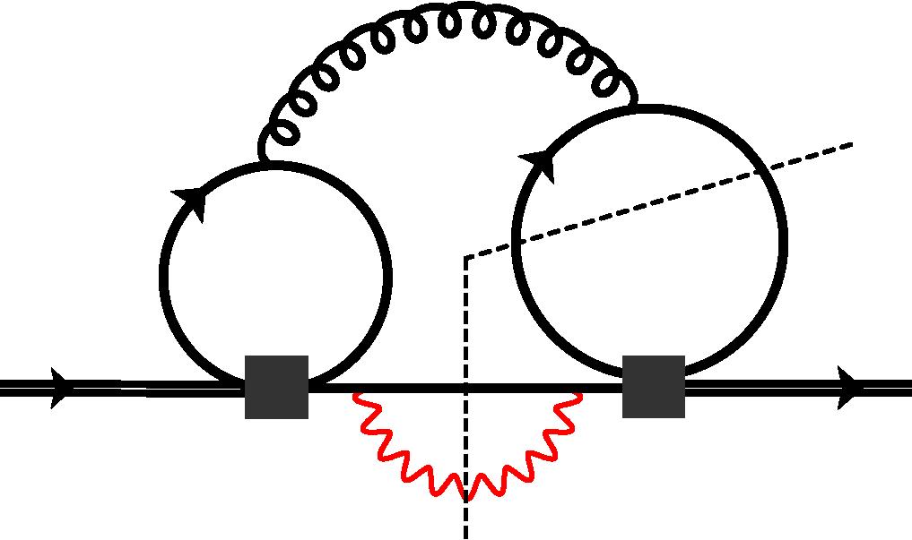
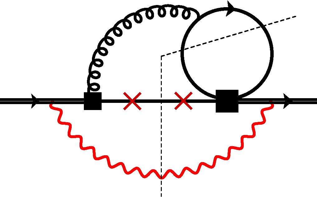
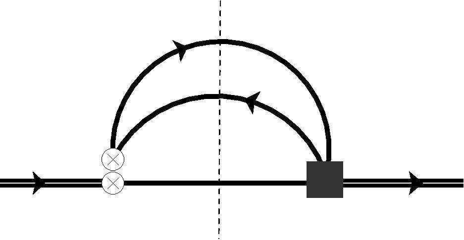
Evaluation of the cut-diagrams shown in Figs. 2, 3, 4. We use the Cutkosky rules for cut (on-shell) propagators, accounting for spin and color sums for all external particles. The result of each diagram is a contribution to the differential decay rate , a scalar function of the momentum invariants , , with (see Sections 2.4 and 2.3.2).
-
2.
Integration over the four-particle phase-space. This step is described in Section 2.4.
- 3.
-
4.
Collinear logarithms: Having regularized collinear divergences in dimensional regularization, we use the method of splitting functions 1209.0965 ; 9605323 ; 0011222 ; 0107138 ; 0301047 to transform poles into collinear logarithms of the form . This requires the computation of the corresponding corrections with subsequent photon emission (with ), by evaluation of the diagrams shown in Fig. 6, the convolution with the splitting function, and the three-particle phase-space integration. This step is described in Section 2.6.
We note that every diagram has to be computed inserting all the operators to the right of the cut, and to the left (see e.g. Fig. 1), leading to all the different interference terms in the matrix . In Section 2.1 we argue that most of the elements of this matrix can be obtained from a reduced set by the use of different operator relations and Fierz identities. In addition, this spells out transparently the dependence of the full result on the Wilson coefficients before any calculation is performed. We will see that – with one exception discussed at the end of Section 2.1.3 – only diagrams with to the left of the cut and to the right must be considered. This simplifies the calculation considerably.
Finally, for each diagram in Figs. 26, there is the corresponding mirror image. These “mirror” contributions are just obtained by complex conjugation, and ensure that the rate is real, i.e. is hermitian. We disregard these mirror contributions in the calculation, but at the end we substitute .
2.1 Operator identities
2.1.1 Color
Diagrams with insertion of the color octet operators are related to the ones with insertion of color singlet operators by a simple color factor, which can be obtained just from the color structure of the gluon penguin:
| (12) |
| (13) |
This leads to the rule that can always be replaced by:
| (14) | |||||
| (15) |
For the same reason, one can always put , meaning that always come in the combination .
2.1.2 Insertions to the right of the cut
We restrict ourselves here to the insertion of operators to the right of the cut. Using the 4D identity we find:
| (16) |
where . We now consider the following “crossed” insertion of into a massless fermion loop with an arbitrary number of vector currents:
| (17) |
There is always an even number of gamma matrices to the left of , which can be moved besides the projector . After that, the relationship provides the given negative sign.
The “straight” insertion of does not vanish in general but does not contribute in our case: In the situation where one vector current is attached to the loop (Fig. 2), the result is proportional to , but there are not enough independent momenta to be contracted with the antisymmetric tensor, so this contribution vanishes. This is true also in the case where the photon couples twice to the quark loop (Fig. 4). In the case of two current insertions (Fig. 3) the result is non-zero, but summing over quarks in the loop the result is proportional to .
Summing up, in the diagrams with a insertion one can always substitute:
| (18) |
The replacement rules (18) combined with Eqs. (14) and (15) imply that the full contribution from can be obtained from the terms proportional to :
| (19) | |||||
| (20) |
Since this is based on a 4D identity, it is in principle only true up to evanescent terms. Below we show that up to the needed order in these terms do not contribute. We have also checked this by direct computation.
The (crossed) insertion of the operators can also be obtained from by an argument almost identical to that of Eq. (17). In this case one must pay attention to the case where the photon couples to the loop, where the and contributions are proportional to different charge factors.
2.1.3 Insertions to the left of the cut
We have shown that we only need to compute diagrams with an insertion of to the right of the cut. To the left of the cut we must insert as well as and . As before, contributions are related to by a simple color factor. In addition, the contribution from is obtained from the insertion with the replacement . We now show that insertions of are also known from the insertions of , and .
First we consider the case of the photon penguin, where the gluon does not couple to the fermion loop to the left of the cut. By direct inspection be find that:
| (21) |
where is the usual “effective” Wilson coefficient 9711280 , which includes the contributions from -quark loops. The corrections are irrelevant to our calculation as the contributions from are finite. The term denotes the contribution from four-quark operators proportional to the structure . This last term does not contribute in our case. To see this, consider the insertion of into the full diagram:
| (22) |
Here the gluon is attached to either ‘’. Since we cut the photon propagator, the photon is on-shell but there is no denominator, and therefore the term cancels. The term also cancels due to the Ward identity . Note that non-zero contributions to the Ward identity vanish since they either involve a massless fermion tadpole, or if the gluon couples to the loop then it does not depend on the incoming/outgoing quark momenta. We have also checked this result by explicit computation, and indeed the different sets of diagrams satisfying the Ward identity vanish identically.
To summarize: all contributions from photon penguins to the left of the cut are obtained from the diagrams with insertion of by the replacement .
Next, we consider the case of the gluon penguin, where the photon does not couple to the fermion loop to the left of the cut. We find:
| (23) |
where , as usual (e.g. Ref. 0203135 ). As before, corrections to the chromomagnetic contribution are irrelevant for our calculation because contributions from are UV-finite (collinear divergences are inconsequential here). In the last term, the quantity is given by:
| (24) | |||||
where is the number of light flavors and
| (25) |
is the loop integral to all orders in . Therefore, all contributions from gluon penguins to the left of the cut are known from the contribution of and .
Now we consider the case in which both the photon and the gluon couple to the loop:
| (26) | |||||
When inserted into the full diagrams, these contributions are both UV-finite and collinear safe222 We consider always the sum of the two diagrams obtained by swapping the gluon and photon insertions. , and we can use 4D identities. The first term in the right-hand side of Eq. (26) can be written as , which defines the function . The second term can be obtained from the first term by the replacement : . The third term () contains only the insertion of , because insertions are zero due to color, while the insertion of vanishes due to Furry’s theorem. For we can make use of the Fierz identity333Here we use the notation , etc.:
| (27) |
which implies that we can trade the straight insertion of with the crossed insertion of . Note also that the contributions from add up to zero in the massless limit due to electric charge: . This means that the third term in Eq. (26) is given by .
The fourth term can be obtained from the first one using the identities in Eqs. (16) and (17), leading to: . The fifth term cannot be completely determined from the insertion of due to the chirality structure. Using the Fierz identity (16) we can trade . The second piece, together with the corresponding contribution from , results in . The rest will provide a term , where . Altogether, the right-hand side of Eq. (26) can be written as:
| (28) |
Therefore only diagrams with insertions of the operators and to the left of the cut need to be calculated, plus the extra contribution from . All these relationships shape the structure of the full results displayed below in the following sections.
2.2 Set of Diagrams
There are three types of diagrams:
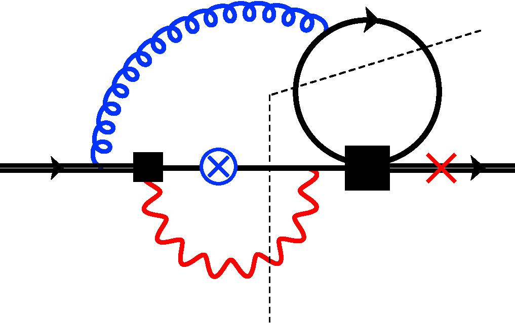
Type (i): The photon does not couple to the cut fermion loop (Fig. 2): In this case crossed and straight diagrams contribute. In addition, straight diagrams contain a factor . All in all, the contribution from these diagrams is:
| (29) |
where and denote the contributions to interference terms
from straight and crossed insertions of the operator to the right of the cut, to diagrams of type , respectively.
Type (ii): The photon couples to the cut fermion loop once (Fig. 3): In this case the straight diagrams are proportional to and need not be considered. The contributions are proportional to . Therefore the total contribution from these diagrams is:
| (30) |
Type (iii): The photon couples to the cut fermion loop twice (Fig. 4): In this case crossed diagrams are proportional to (or in the case of ) and straight diagrams to . We have:
| (31) | |||||
We assume that the objects are phase-space-integrated matrix elements containing no prefactors or couplings, such that:
| (32) |
in the notation of Eq. (9). In Eq. (32), denotes the UV counterterms, and both include the relevant collinear counterterms. Both are discussed below in Sections 2.5 and 2.6. The structure of the objects can be deduced from the discussion in Section 2.1.3. In the case of we have:
| (33) |
For we have:
| (34) |
| (35) |
where . The contributions with penguin operators to the left of the cut are given by:
| (36) | |||||
The functions include the collinear regulators discussed in Section 2.6. The functions and are related to diagrams where the photon couples to the left-hand quark loop, corresponding respectively to the terms with and in Eq. (28). Explicit results for all these functions are collected in Appendix A.
2.3 Other details
2.3.1 Irrelevance of evanescent terms to the right of the cut
In the case of interference, there are no UV or collinear divergences, and therefore evanescent structures are irrelevant for the result.
In the case of interference, collinear divergences appear which combined with evanescent terms give finite contributions in the dimensionally regularized result. However these finite terms cancel when we express the dimensional regulators in terms of logarithms of masses, via the splitting-function approach (see Section 2.6):
| (37) |
since the terms cancel in both 4D and evanescent terms separately.
In the case of interference, UV and collinear divergences are nested inside dimensionally regularized expressions. However all UV divergences cancel against counterterm diagrams, including finite terms from evanescent operators:
| (38) |
All “finite” terms from collinear divergences now disappear when going to mass regularization, as in the case with .
2.3.2 Cancellation of terms
Traces with will introduce terms proportional to in the differential decay rate. Here we show that these terms always cancel if we perform a full angular integration over phase-space.
Consider fixing all double invariants . Then all are fixed only up to an Euler rotation and an orientation. To see this go to the rest frame of the -quark. Momentum conservation fixes all the energies (since are fixed). This implies that are also fixed. We can rotate the frame to put along the positive axis, and in the plane. Then is fixed only up to a two-fold ambiguity (an orientation), given by the sign of its component. Once this sign is chosen is also fixed. This proves that is fixed by up to a sign, which is given by the orientation of .
Now consider phase-space integration. Terms in the integrand of the form do not depend on the Euler rotation nor the orientation, and the angular integral over can always be performed trivially, giving a factor . Terms of the form , however, change sign under change of orientation, and vanish upon integration over . Obviously parity-odd terms cancel out in parity-even observables. Therefore we drop these terms from the beginning in the calculation of the integrated decay rate.
2.4 Phase-space integration
The phase-space measure for a () decay of a particle of mass into four massless particles with momenta is given in terms of kinematic invariants by 0311276 :
| (39) | |||||
where (), and is the Gram determinant:
| (40) |
The unpolarized decay rate is given by the phase-space integral:
| (41) |
where the sum runs over the spins and color of all particles (we assume the parent is a color triplet). depends only on : , so the angular integrations can be performed trivially:
| (42) |
and the general formula for the decay rate becomes
| (43) |
This integral might contain soft and/or collinear divergences associated to regions of phase space where some particles are soft or collinear. These divergences can be regularized in dimensional regularization by setting . If we insist on integrating over these regions, one must include virtual corrections to cancel the divergences. Otherwise, the regulator must be traded by a physical cutoff at a later stage.
We now specify to the case. We consider a cut on the photon energy (in the quark rest frame), which defines the parameter . This translates into the constraint , which can be included in the phase-space integral in the following way. We include a delta function in the integrand, and we integrate over the new variable from to :
| (44) |
The delta functions can be used to integrate over two invariants, e.g. and :
| (45) |
where , and is given by the prefactor in Eq. (43), and the substitution rule corresponds to and . The next integration can be performed over an invariant that appears only polynomially in (see e.g. 0512066 ). It is easy to see that always satisfies this criterion by checking the uncut propagators in Figs. 2,3,4 and the loop functions. Upon substitution of , the Gram determinant remains quadratic in : , where are complicated functions of the rest of the invariants:
| (46) | |||||
| (47) |
Thus, is positive only if are real (happening only if ), and for . In addition, . This sets the integration limits for and imposed by the -function, which can then be dropped:
| (48) |
Now it is convenient to perform the following changes of variables:
| (49) |
where are integrated independently from 0 to 1, and
| (50) | |||||
| (51) |
This gives
| (52) | |||||
In the following we must consider the kernel . As mentioned above, is polynomial in : . Expanding according to (49)-(51) will provide a sum of terms of the form
| (53) |
and the integral over the variable gives a factor for each term. The next steps depend on the diagram at hand. Consider the diagrams with . In this case,
| (54) |
for some . The integral over gives again a -function: . Because of the and factors, the next steps will introduce hypergeometric functions. The integral over gives
| (55) |
and the integral over , gives:
| (56) |
The next step is to expand around (with ). The expansion of hypergeometric functions is performed automatically by the package HypExp HypExp . This will give finite results in the case of , but poles in the case of , corresponding to collinear divergences. The integration over the photon energy can then be performed, also analytically, for all terms.
The case of loop diagrams is in principle more complicated, as the function contains already a hypergeometric function. For instance, in the case of diagrams (i) with the photon not attaching to the quark loop, the variable appears in the function (cf. Eq. (25)). However, by a suitable choice in the order of integration, analytic results can be obtained as before. In the case of diagrams such as (iii), the hypergeometric function depends on the triple invariant , and the sequential-integration procedure described above does not seem to work up to finite order in . In this case we extract all the and poles analytically and leave the finite terms differential in one of the variables, which we integrate numerically afterwards. This is also the case for the diagrams where the photon couples to the charm loop, which are both UV and collinear finite. In general, for the loop contributions, some finite terms turn out to be complicated functions of and . We give these results as polynomial expansions in around the physical value . The coefficients of this expansion are presented as numerical interpolations in the variable , reproducing the exact results to enough precision for all practical purposes. We have checked that the interpolated expressions in the appendix reproduce the exact results with high precision in the full range for values of near .
2.5 Renormalization
Tree-level four-body contributions from four-quark operators arise at LO in and have been computed in Ref. 1209.0965 . At NLO the corresponding counterterm contributions must be included, which cancel the UV divergences from the loop diagrams. One must consider the insertion of the bare operators , , in the tree-level diagrams to the left of the cut, where:
| (57) | |||||
The first term leads to the LO contributions in Ref. 1209.0965 , while the second term contributes to the NLO result and takes care of the UV divergences. For this we need, a priori, the tree level results with including terms, and the renormalization factors .
The relevant renormalization factors are simple to compute. Using the relationships developed in Section 2.1, and expressing the result in terms of tree-level matrix elements of four-quark operators, we find that:
| (58) |
This fixes the renormalization factors needed in our calculation:
| (59) |
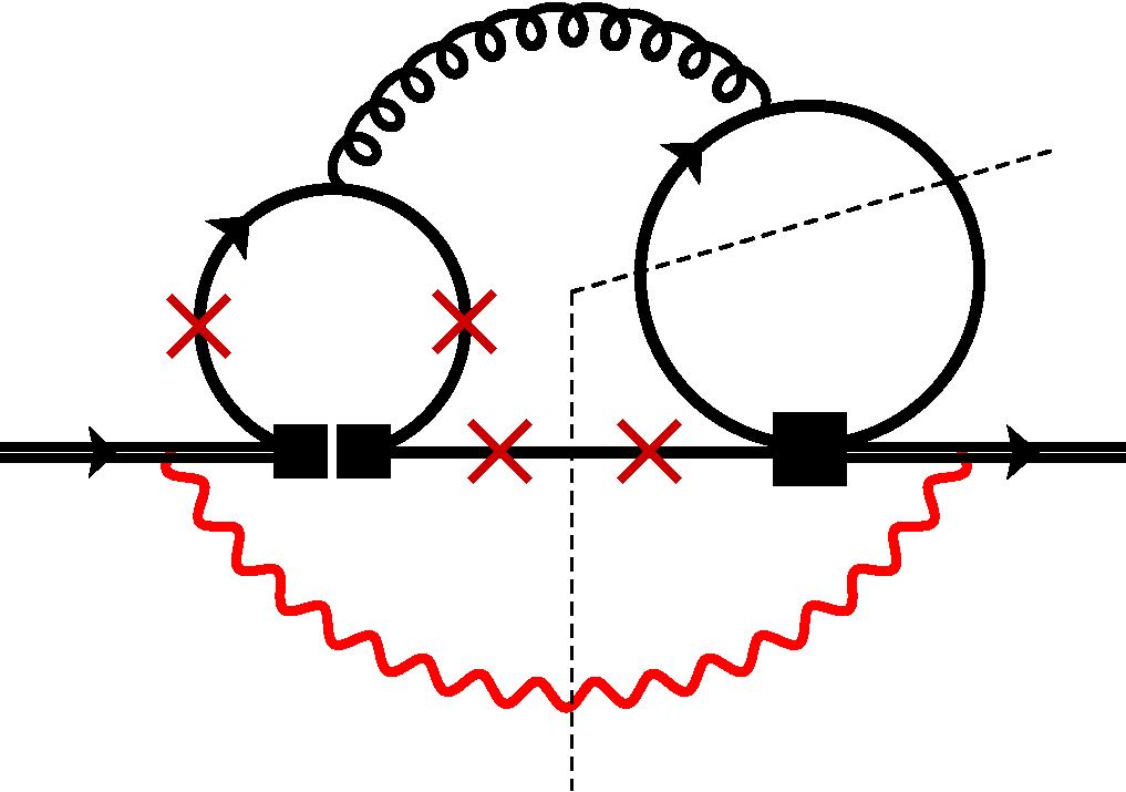
We also see that we need only tree level diagrams with insertion of to the left of the cut. All the diagrams needed are shown in Fig. 5.
For the operator insertions to the right of the cut we can (and must) use the 4D identities derived in Section 2.1, noting that evanescent terms cancel in the renormalization process by virtue of Eq. (38). This leads to exactly the same structure as Eqs. (29),(30),(31) for the counterterm diagrams (i.e. Eq. (32)), with the corresponding matrix elements given by:
| (62) | |||||
Again, . The functions are given in Appendix A. One can check that all UV divergences cancel, as expected: .
2.6 Collinear divergences and splitting functions
The region of phase space in which the photon is collinear to one of the light quarks gives rise to collinear divergences. These divergences are regulated dimensionally in our computation. However, these are just artifacts of the massless limit used for light quarks, and there is a more natural regulator: a physical cut-off given by the light meson masses. A suitable parametrization of such (near-) collinear effects consists in keeping the light quarks massive and perform a massive phase-space integration. This is quite complicated from the practical point of view, taking into account that the massless phase-space integrals computed here are already rather challenging.
Fortunately, one may resort to the factorization properties of the amplitudes in the quasi-collinear limit (see e.g. 1209.0965 ). The idea is that close to the collinear region, the amplitude may be expressed as a amplitude times a splitting function , describing the quasi-collinear emission of a photon from , summed over . The splitting functions encode the collinear divergences, and can themselves be regulated by quark masses or in dimensional regularization. Both approaches are rather simple, since in this limit the four-body phase space factorizes into a convolution of the three-body phase space of the non-radiative process and the phase space of the radiative process alone: . By comparing the splitting functions regulated in these two different schemes, one can write a formula to switch from one to the other at the level of the decay rate 1209.0965 :
| (63) |
where
| (64) | |||||
Here is the spin-summed squared matrix element of the decay obtained by evaluating the diagrams in Fig. 6, and is the three-particle phase-space measure in dimensions 0311276 :
| (65) | |||||
Integrating Eq. (64) over provides the terms contained in the functions . The contributions from the chromomagnetic operator (Fig. 6, left) enter into Eq. (33). The contributions from four-quark operators (Fig. 6, center) go into Eqs. (34), (35) and (36). The counterterm contributions (Fig. 6, right), enter into Eq. (62). The functions are collected in Appendix A.
One can check that adding the collinear contribution removes the terms that survive the renormalization process, trading them for collinear logarithms of quark-mass ratios. These collinear logarithms are of the form , with . The quark masses are collinear regulators and it is difficult to relate them to physical masses. In our numerical analysis we will take a common constituent-quark mass MeV for all three light flavors, and use the notation . This should provide a reasonable estimate of the effect of collinear logarithms.
3 Results
We write the four-body contribution to the rate as:
| (66) |
where is the absolute normalization of the decay rate:
| (67) |
The sum runs over . The Wilson coefficients are real, but contain CKM phases:
| (68) |
with the Wilson coefficients in the notation of Ref. 9612313 . They are needed here to NLO:
| (69) |
their numerical values are given below.
The matrix elements depend on the renormalization scale and the photon-energy cut and can be split into LO and NLO components:
| (70) |
The LO matrix is real and symmetric and was computed in Ref. 1209.0965 : we reproduce and confirm these results (after the 2014 update of that paper). We write (here ):
| (71) |
where:
| (72) | |||||
| (73) | |||||
| (74) | |||||
The NLO matrix contains perturbative strong phases from on-shell contributions from light quarks, as well as from charm quarks when the photon-energy cut is low enough. The matrix is the main result of this paper. It has the following structure:
| (75) |
where , and . The explicit form of is too complicated to be written down here. However, it can be constructed completely from the expressions in Sections 2.2, 2.5 and Appendix A: Start from Eq. (32), substitute the objects from Eqs. (29), (30), (31), then use Eqs. (33)-(36) and (62) for the different matrix elements , and use the expressions in the appendix for the functions , and , noting that . Finally, perform the replacement to account for the “mirror” contributions. For convenience, we provide the full matrices and in the file “Gij.m” attached to the arXiv submission of the present manuscript. The first is given by the matrix “GijLO” () and the second by the matrix “GijNLO” (with ).
4 Numerical analysis
We briefly discuss here the numerical impact of the four-body contributions to the total rate. We consider for convenience the following quantity:
| (76) |
given by Eq. (66) and normalized to the leading contribution to the decay rate. The Wilson coefficients are given by:
| (77) |
which are computed following Ref. 9910220 . For the reference matching and renormalization scales GeV, GeV, we have444 The NLO Wilson Coefficients are not needed for our NLO results as do not contribute at LO. :
| (78) | |||||
| (79) |
for . However, the -dependence of the Wilson coefficients is important and we will analyze it here. In addition, denote the appropriate CKM factors, given by pdg :
| (80) |
The quantity can be expanded in :
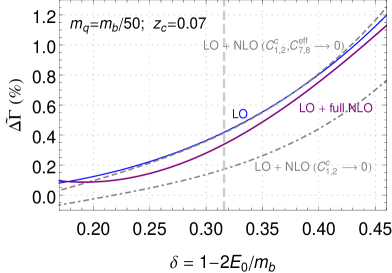
We begin with a discussion of the -dependence of our results. To leading order, the -dependence is given purely by the LL (leading-log) running in the effective theory. Note that to this order, only and contribute. At NLO, three new contributions arise: (i) the contribution from NLO Wilson coefficients, (ii) NLO matrix elements and (iii) contributions from , absent at LO. The -dependence should cancel up to a residual scale-dependence from higher orders, and up to the neglected contributions shown in Fig. 1.f (note that the factors in Eq. (59) are not the full renormalization constants).
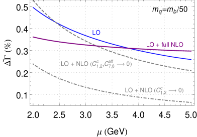
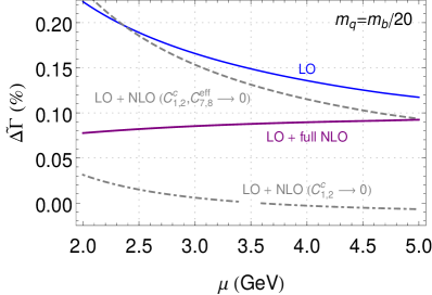
In Fig. 7 we show the -dependence of the LO result, and LO+NLO excluding , LO+NLO excluding and LO+ full NLO. We also gauge the impact of collinear logarithms, showing the result for two different choices of , corresponding to ( MeV) and ( MeV). Collinear logarithms are, as expected, numerically important.
Contributions from and arise only at NLO and therefore introduce at this order a novel -dependence. Although, as we will see, certain cancellations make the NLO contribution small, there is a considerable reduction in the renormalization-scale dependence of the full LO+NLO result as compared to the LO contribution alone. This is due to the fact that the main -dependence of the leading order contribution arises from the mixing of onto penguin operators, which is compensated at NLO by the matrix elements of . This can be seen in Fig. 7: the reduction in the -dependence is achieved only after including contributions.
In the left plot of Fig. 7 one can see that for the value GeV strong cancellations make the NLO contribution very small. More concretely, for the inputs GeV, GeV, , and , we have:
| (82) | |||||
where the term labeled ‘NLO WCs’ corresponds to the second term in Eq. (4). This cancellation is very efficient for GeV, but depends strongly on and . However, it is a general feature of our results that the contribution from is of the same order as the rest of the NLO contribution, but with opposite sign, leading always to some level of cancellation. Note also that the (NLO) contribution is also as large as the LO result.
In the following we fix the renormalization scale to GeV and study the dependence on the charm mass and the photon-energy cut. This is shown in Fig. 8. In general the full LO+NLO result increases with and decreases with , always remaining below the level for . We note that these results are only valid for not far from as some of the functions are expanded up to second order in .
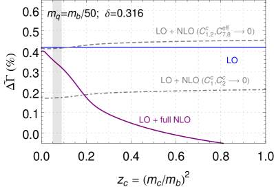
Finally, we provide some results for two different values of of interest: GeV, corresponding to ,
and GeV, corresponding to . For the input parameters and their uncertainties we take:
, and , which captures the different values for
within different schemes.
For MeV, we find:
| (83) | |||||
| (84) | |||||
For MeV:
| (85) | |||||
| (86) | |||||
For the value ( GeV) we have used the exact results (not the expanded ones), as for this value of the quadratic expansion is not expected to be accurate enough.
5 Conclusions
The inclusive radiative decay has beyond any doubt reached the era of precision physics, with the total uncertainties on both the experimental and theoretical side being at the level. The foreseen improvement in precision on the experimental side – the envisaged uncertainty with ab at Belle II is of 1011.0352 , although this might even be a conservative estimate – justifies every effort to reduce the theoretical error to at least the same level.
The present article aims at addressing a particular higher-order perturbative contribution, namely the four-body contributions to at NLO. The smallness of the Wilson coefficients of penguin operators and CKM-suppression of current-current operators suggests that this contribution should be small. However, only an explicit calculation can turn this estimate into a firm statement. The calculation arises from tree and one-loop amplitudes, but it involves the four-body phase-space integration in dimensional regularization, which makes the calculation non-trivial owing to the appearance of higher transcendental functions. Moreover, the cancellation of poles in the dimensional regularization parameter is only achieved after proper UV and IR renormalization. The latter gives rise to logarithms when turning the dimensional into a mass regulator. These logarithms stem from the phase space region of energetic collinear photon radiation off light quarks in the final state. They are computed with the splitting function technique and treated in the same way as in 0512066 ; 1209.0965 .
We find indeed that the contribution of our four-body NLO correction to the total rate is below the level, as expected. This statement even holds true once we vary the input parameters such as the charm mass , the photon energy cut (parameterized by ), the masses of the light quarks, or the renormalization and matching scales, as can be seen by the numbers and the plots in Section 4. We also confirm the LO results presented previously in Ref. 1209.0965 .
Yet the NLO calculation of is still not complete. There are certain yet unpublished three-particle cuts contributing to , mainly interferences of with , which are also of the -interference type. These contributions can be extracted from the results of Ref. 9512252 . The only missing pieces are given by the diagrams in Fig. 1.f. These are NLO interferences of the type and are expected to be negligible with respect to the ones that we have calculated in a complete manner. While these contributions can be calculated with the techniques described in this paper, they are left for future work.
Acknowledgements
We thank Mikolaj Misiak for valuable correspondence and comments on the manuscript, and Dirk Seidel for useful discussions about penguins. This work has been funded by the Deutsche Forschungsgemeinschaft (DFG) within research unit FOR 1873 (QFET). M.P. acknowledges support by the National Science Centre (Poland) research project, decision DEC-2011/01/B/ST2/00438.
Appendix A Intermediate Results
A.1 interference
The functions are given by:
| (87) | |||||
| (88) | |||||
| (89) |
A.2 interference
Up to subleading terms in , we have always
| (90) |
The functions are given by:
| (91) | |||||
| (92) | |||||
| (93) | |||||
| (94) | |||||
| (95) |
where and , and:
| (96) | |||||
| (97) | |||||
| (98) | |||||
| (99) | |||||
| (100) | |||||
| (101) | |||||
| (102) | |||||
A.3 interference
For we give analytical results for -independent functions, but the -dependence is given as interpolated functions. Up to subleading terms in , we have always
| (103) |
The functions are given by:
| (104) | |||||
| (105) | |||||
| (106) | |||||
Counterterms are given by:
| (109) | |||||
| (110) | |||||
| (111) | |||||
| (112) | |||||
| (113) | |||||
where again and . From these expressions one can check the pattern of cancellation of UV and collinear divergences. The -independent functions are given by (with the notation , , ),
| (114) | |||||
| (115) | |||||
| (116) | |||||
| (117) | |||||
| (118) | |||||
| (119) | |||||
| (120) | |||||
| (121) | |||||
| (122) | |||||
| (123) | |||||
| (124) | |||||
| (125) | |||||
| (127) | |||||
While our calculation provides exactly all the functions , and , the corresponding expressions depend on and the photon energy through complex functions of harmonic polylogarithms of various weights, which must be integrated in the region . Solving these integrals analytically is highly non-trivial, and even the numerical integration is computationally demanding. We have performed a numerical evaluation of such integrals and find it more convenient to present the results as an expansion in around the value , and as an interpolation in . These interpolations coincide with the exact results in the region to a very good precision. The relevant functions are written as:
| (128) | |||||
with . The functions , are fitted to padé approximants of order :
| (129) |
and similar for . The Padé coefficients are given in Tables A.3-A.3.
Table 1. Padé coefficients for .
| {5} | 2.6085e2 | -2.3748e3 | 7.8427e2 | -2.5964e0 | -1.8780e1 | -7.0839e1 |
| {4} | 5.5417e2 | 1.6248e2 | 8.9587e2 | 3.6935e0 | 2.6299e1 | 8.9418e1 |
| {3} | -8.6141e0 | 1.2216e3 | -2.0894e2 | -1.6902e0 | -1.1864e1 | -3.5637e1 |
| {2} | -1.5107e0 | -9.2378e1 | 2.1731e1 | 3.2301e-1 | 2.2545e0 | 6.0307e0 |
| {1} | 1.1241e-1 | 5.4522e0 | -1.3841e0 | -2.6875e-2 | -1.8840e-1 | -4.5543e-1 |
| {0} | 3.2101e-3 | 2.0675e-2 | 4.0727e-2 | 8.0387e-4 | 5.7122e-3 | 1.2664e-2 |
| {-1} | 2.7478e1 | 2.4959e2 | -3.5865e1 | 5.1543e0 | -9.6139e0 | -2.1925e1 |
| {-2} | -6.5543e1 | -4.3377e3 | 5.9242e2 | -2.5093e2 | -1.8937e2 | -1.6101e2 |
| {-3} | -9.6131e3 | 5.7863e4 | -5.6283e3 | 1.7465e4 | 1.1349e4 | 1.1056e4 |
| {-4} | 2.2612e5 | 7.7096e4 | 2.1131e4 | -4.3025e5 | -2.3262e5 | -1.5200e5 |
| {-5} | 1.6782e5 | -2.0939e5 | 3.8351e4 | 4.3797e6 | 1.7123e6 | 7.2442e5 |
Table 2. Padé coefficients for .
| {5} | -9.5739e-1 | -9.6422e0 | -2.8386e1 | -7.9067e-2 | -6.6893e-1 | -2.9051e0 |
| {4} | 3.0239e0 | 2.7036e1 | 1.2991e2 | 1.9267e-1 | 1.6095e0 | 6.3544e0 |
| {3} | -3.9058e-1 | -6.8880e-1 | 2.3899e0 | -1.7623e-1 | -1.4512e0 | -5.1486e0 |
| {2} | 3.7847e-3 | -6.4972e-1 | -4.0154e0 | 7.5813e-2 | 6.1479e-1 | 1.9516e0 |
| {1} | -9.5759e-3 | 3.6265e-3 | 2.4684e-1 | -1.5417e-2 | -1.2304e-1 | -3.5068e-1 |
| {0} | 3.9641e-3 | 3.0018e-2 | 7.5378e-2 | 1.1925e-3 | 9.3670e-3 | 2.4204e-2 |
| {-1} | -4.6336e0 | -2.3791e0 | 2.8343e-1 | -7.6041e0 | -6.7239e0 | -5.9052e0 |
| {-2} | 3.1991e1 | 1.5265e1 | -1.9554e0 | 5.0750e1 | 4.1512e1 | 2.0995e1 |
| {-3} | -2.6083e2 | -2.3013e2 | -3.0385e2 | -1.6999e2 | -8.9622e1 | 2.8933e2 |
| {-4} | 1.1184e3 | 1.4088e3 | 2.6697e3 | -2.6338e2 | -7.5669e2 | -4.3799e3 |
| {-5} | -3.1470e2 | -4.4778e2 | -4.4635e2 | 3.2029e3 | 5.1645e3 | 1.9822e4 |
Table 3. Padé coefficients for .
| {5} | 6.7269e2 | 4.9426e2 | 1.0451e3 | -3.4512e1 | -2.3670e2 | -9.4447e2 |
| {4} | 3.3679e3 | 5.8344e3 | 3.4974e3 | 4.8342e1 | 3.2457e2 | 1.1315e3 |
| {3} | 2.3178e2 | 2.4369e2 | -6.8258e2 | -2.1749e1 | -1.4292e2 | -4.2386e2 |
| {2} | -3.3437e1 | -8.0765e1 | 7.0897e1 | 4.0984e0 | 2.6571e1 | 6.7645e1 |
| {1} | 1.7801e0 | 2.8034e0 | -5.3246e0 | -3.3765e-1 | -2.1805e0 | -4.8418e0 |
| {0} | 1.8570e-2 | 1.0740e-1 | 1.8133e-1 | 1.0040e-2 | 6.5154e-2 | 1.2819e-1 |
| {-1} | 7.1021e1 | 1.0292e1 | -3.4108e1 | 9.6116e0 | -8.1610e0 | -2.2268e1 |
| {-2} | -6.9880e2 | -1.5360e2 | 5.3644e2 | -6.8385e2 | -3.9083e2 | -2.5150e2 |
| {-3} | -5.9528e3 | -6.3499e3 | -5.0770e3 | 3.0179e4 | 1.5933e4 | 1.3515e4 |
| {-4} | 3.3626e5 | 9.9501e4 | 2.0032e4 | -6.1404e5 | -2.6974e5 | -1.6966e5 |
| {-5} | 1.9465e5 | 4.3193e4 | 3.0917e4 | 5.0960e6 | 1.7175e6 | 7.4113e5 |
Table 4. Padé coefficients for .
| {5} | 3.7841e2 | 5.9118e2 | 3.9056e2 | -4.5121e-1 | -6.0463e1 | -2.1698e1 |
| {4} | 2.7044e2 | 4.8884e2 | 5.4690e2 | 7.9268e-1 | 8.8873e1 | 3.5043e1 |
| {3} | -1.1579e2 | -1.8312e2 | -1.8791e2 | -5.0952e-1 | -3.9767e1 | -1.8854e1 |
| {2} | 1.3594e1 | 1.9867e1 | 2.5682e1 | 1.5463e-1 | 5.9243e0 | 4.2454e0 |
| {1} | 3.0297e-2 | -1.6165e-1 | -1.7434e0 | -2.2768e-2 | -1.7640e-1 | -4.0900e-1 |
| {0} | 5.8184e-3 | 3.5538e-2 | 5.7703e-2 | 1.3344e-3 | 8.5805e-3 | 1.5244e-2 |
| {-1} | 1.4953e0 | -7.2811e0 | -3.1995e1 | 1.1886e1 | -8.8975e0 | -2.7485e1 |
| {-2} | 2.4503e3 | 6.0955e2 | 4.7985e2 | -5.2688e2 | 4.2689e2 | 3.3788e2 |
| {-3} | -1.9815e4 | -5.2682e3 | -3.4156e3 | 5.3900e3 | 1.1219e4 | -9.5618e2 |
| {-4} | 3.7632e4 | 1.1781e4 | 8.8305e3 | -2.3444e4 | -1.4783e5 | -1.2086e4 |
| {-5} | 1.0249e5 | 2.6408e4 | 1.1136e4 | 3.8372e4 | 5.4497e5 | 8.0691e4 |
Table 5. Padé coefficients for .
| {5} | -7.7072e0 | -7.3684e1 | -3.2672e2 | -8.7364e-1 | -6.3940e0 | -3.5367e1 |
| {4} | 6.5728e0 | 3.6241e1 | 1.4444e2 | 2.0978e0 | 1.5469e1 | 7.3871e1 |
| {3} | 4.6807e0 | 7.0186e1 | 3.8320e2 | -1.8917e0 | -1.4054e1 | -5.6847e1 |
| {2} | -1.5486e0 | -1.9670e1 | -9.3766e1 | 8.0372e-1 | 6.0118e0 | 2.0476e1 |
| {1} | 1.0573e-1 | 1.6449e0 | 8.0166e0 | -1.6179e-1 | -1.2175e0 | -3.5220e0 |
| {0} | 1.8873e-2 | 1.3658e-1 | 3.3186e-1 | 1.2423e-2 | 9.3960e-2 | 2.3583e-1 |
| {-1} | -4.4964e-1 | 4.8147e0 | 1.4577e1 | -6.6212e0 | -4.6773e0 | -2.9278e0 |
| {-2} | -2.5309e0 | -4.5104e1 | -1.3130e2 | 2.2861e1 | -8.8411e0 | -7.8932e1 |
| {-3} | -1.7756e2 | -5.9658e1 | 1.1661e2 | 1.0154e2 | 4.6805e2 | 1.6895e3 |
| {-4} | 1.3958e3 | 1.8710e3 | 3.9334e3 | -1.5110e3 | -3.7935e3 | -1.3934e4 |
| {-5} | -1.0185e3 | -1.5684e3 | -3.2201e3 | 5.1086e3 | 1.1386e4 | 4.4771e4 |
Table 6. Padé coefficients for .
| {5} | 6.4806e1 | 3.5981e2 | 1.2940e2 | 2.1801e1 | 1.5065e2 | 6.3214e2 |
| {4} | -8.5279e2 | -1.5483e3 | -1.4843e3 | -3.0643e1 | -2.0732e2 | -7.5761e2 |
| {3} | -9.9349e1 | -4.0637e2 | 2.2130e2 | 1.3820e1 | 9.1544e1 | 2.8342e2 |
| {2} | 1.2871e1 | 6.1243e1 | -2.0763e1 | -2.6077e0 | -1.7054e1 | -4.5145e1 |
| {1} | -5.9578e-1 | -2.2780e0 | 1.9360e0 | 2.1490e-1 | 1.4015e0 | 3.2245e0 |
| {0} | -7.3348e-3 | -4.1945e-2 | -7.8462e-2 | -6.3860e-3 | -4.1912e-2 | -8.5194e-2 |
| {-1} | 4.7343e1 | 2.3190e1 | -3.2893e1 | 1.4649e1 | -3.5937e0 | -1.8952e1 |
| {-2} | -1.4068e2 | -3.0228e2 | 5.2625e2 | -7.6567e2 | -5.4265e2 | -3.8314e2 |
| {-3} | -1.3594e4 | -7.1646e3 | -5.3673e3 | 3.2909e4 | 1.9737e4 | 1.5799e4 |
| {-4} | 3.2738e5 | 1.3102e5 | 2.2555e4 | -6.6974e5 | -3.2807e5 | -1.9062e5 |
| {-5} | 2.8262e5 | 4.3433e4 | 3.7019e4 | 5.6997e6 | 2.0888e6 | 8.2259e5 |
Table 7. Padé coefficients for .
| {5} | -2.7046e1 | -1.1652e2 | -6.3378e3 | 4.8640e-1 | 3.9114e0 | 1.7243e1 |
| {4} | -4.2392e2 | -4.6203e3 | -5.8000e4 | -1.1720e0 | -9.3898e0 | -3.7292e1 |
| {3} | 1.3189e2 | 1.3432e3 | 1.5166e4 | 1.0609e0 | 8.4650e0 | 3.0070e1 |
| {2} | -8.8744e0 | -9.3948e1 | -1.1660e3 | -4.5251e-1 | -3.5954e0 | -1.1478e1 |
| {1} | -1.4275e0 | -1.2464e1 | -8.5821e1 | 9.1466e-2 | 7.2362e-1 | 2.1083e0 |
| {0} | -4.5677e-3 | -3.6869e-2 | -1.1199e-1 | -7.0517e-3 | -5.5554e-2 | -1.5106e-1 |
| {-1} | 2.8279e2 | 3.0406e2 | 7.1445e2 | -7.6394e0 | -6.0846e0 | -4.0315e0 |
| {-2} | -1.2889e3 | -9.3334e2 | 1.1757e3 | 3.3059e1 | 7.5335e0 | -4.7914e1 |
| {-3} | 9.6814e3 | 7.3874e3 | -7.4918e3 | 1.2448e1 | 2.7671e2 | 1.2068e3 |
| {-4} | -7.8680e4 | -8.4193e4 | -1.9839e5 | -1.0211e3 | -2.5305e3 | -1.0096e4 |
| {-5} | 2.9932e5 | 3.9930e5 | 1.7241e6 | 3.8601e3 | 7.8008e3 | 3.2678e4 |
The functions are UV finite and collinear safe. Again, we have the following relationship,
| (130) |
As before, the ‘crossed’ functions are known exactly but we provide here simplified expressions as an expansion in and interpolated in . We write:
| (131) | |||||
with . The functions are again fitted to Padé approximants:
but a different parameterization for the functions is found to reproduce the exact result more accurately. While for and we use
| (133) | ||||
| we make the ansatz | ||||
| (134) | ||||
for . The coefficients and can be found in Tables A.3 and A.3, respectively.
Table 8. Padé coefficients for the real parts of .
| {5} | -6.0396e1 | -7.9313e2 | -4.1781e2 | 8.5226e3 | 5.9559e4 | 6.0577e2 |
| {4} | -4.3337e1 | 4.3943e1 | 1.7075e2 | 5.2397e2 | -1.7693e3 | -2.4607e2 |
| {3} | 2.7398e1 | 7.1810e1 | -2.3013e1 | -6.9260e2 | -2.5828e3 | 4.0981e1 |
| {2} | -4.9232e0 | -1.6196e1 | 1.0162e0 | 1.3412e2 | 5.3783e2 | -3.9970e0 |
| {1} | 1.9455e-1 | 6.9739e-1 | -1.0853e-2 | -3.4138e0 | -1.4094e1 | 2.4014e-1 |
| {0} | 4.7105e-4 | 2.1302e-3 | 4.5410e-4 | -1.5811e-3 | -8.3330e-3 | -5.1000e-3 |
| {-1} | 3.2507e2 | 2.5362e2 | -6.7339e1 | 1.8946e3 | 1.4787e3 | -3.6244e1 |
| {-2} | -1.2129e3 | -3.3619e3 | 2.9914e3 | 2.7983e4 | 1.4145e4 | 1.3530e3 |
| {-3} | 4.5871e4 | 3.7550e4 | -6.7242e4 | 3.3450e5 | -3.5081e4 | -3.2312e4 |
| {-4} | -2.7172e5 | 8.5735e4 | 7.6883e5 | 2.2367e6 | 7.2362e6 | 4.1425e5 |
| {-5} | -3.6784e5 | -2.6336e6 | -4.2134e6 | -4.8970e7 | -7.8826e7 | -2.5466e6 |
| {-6} | 4.8301e6 | 9.5241e6 | 8.8361e6 | 3.1279e8 | 4.0127e8 | 5.9475e6 |
Table 9. Coefficients for the imaginary parts of .
| {6} | 0 | 0 | 2.7269e9 | 3.0740e10 |
| {5} | 0 | 5.9601e5 | -5.6512e8 | -5.4396e9 |
| {4} | -3.4279e4 | -2.5773e5 | 5.1876e7 | 4.4076e8 |
| {3} | 5.4423e3 | 3.5916e4 | -2.2643e6 | -1.6493e7 |
| {2} | -5.0377e2 | -2.5068e3 | 5.7546e4 | 3.7561e5 |
| {1} | 9.7190e0 | 2.9523e1 | -5.7810e2 | -3.0581e3 |
| {0} | -7.3742e-1 | -2.5466e0 | 6.7661e0 | 3.4673e1 |
| {} | 2.9801e1 | 2.3898e1 | 8.2260e1 | 9.3516e1 |
| {7} | 1.9156e7 | 0 |
| {6} | -1.2045e7 | -4.0614e7 |
| {5} | 2.7691e6 | 2.8773e7 |
| {4} | -2.4695e5 | -9.2094e6 |
| {3} | -1.3034e3 | 1.6547e6 |
| {2} | 1.5514e3 | -1.5575e5 |
| {1} | -8.3143e1 | 5.4749e3 |
| {0} | 1.1641e0 | 3.0407e1 |
| {-1} | 5.3853e1 | 1.0191e3 |
| {-2} | -4.7202e3 | 5.4442e3 |
| {-3} | 1.2537e5 | -6.7695e5 |
| {-4} | -1.7062e6 | 1.0194e7 |
| {-5} | 1.2920e7 | -4.8380e7 |
| {-6} | -5.1347e7 | -2.3921e7 |
| {-7} | 8.3239e7 | 4.9141e8 |
Finally the functions are given by
| (135) |
and
References
- (1) CLEO Collaboration, “Branching fraction and photon energy spectrum for ,”, Phys. Rev. Lett. 87, 251807 (2001) [hep-ex/0108032].
- (2) Belle Collaboration, “A Measurement of the branching fraction for the inclusive decays with BELLE”, Phys. Lett. B 511, 151 (2001) [hep-ex/0103042]; “Measurement of Inclusive Radiative B-meson Decays with a Photon Energy Threshold of 1.7 GeV”, Phys. Rev. Lett. 103, 241801 (2009) [arXiv:0907.1384 [hep-ex]].
- (3) BaBar Collaboration, “Measurement of the branching fraction and photon energy spectrum using the recoil method”, Phys. Rev. D 77, 051103 (2008) [arXiv:0711.4889 [hep-ex]]; “Exclusive Measurements of Transition Rate and Photon Energy Spectrum”, Phys. Rev. D 86, 052012 (2012) [arXiv:1207.2520 [hep-ex]]; “Measurement of B(), the photon energy spectrum, and the direct asymmetry in decays”, Phys. Rev. D 86, 112008 (2012) [arXiv:1207.5772 [hep-ex]]; “Precision Measurement of the Photon Energy Spectrum, Branching Fraction, and Direct CP Asymmetry ”, Phys. Rev. Lett. 109, 191801 (2012) [arXiv:1207.2690 [hep-ex]].
- (4) Y. Amhis et al. [Heavy Flavor Averaging Group Collaboration], “Averages of -hadron, -hadron, and -lepton properties as of early 2012”, arXiv:1207.1158 [hep-ex], and online update at http://www.slac.stanford.edu/xorg/hfag.
- (5) Y. Sato, Talk at CKM’2014, “Inclusive decays and exclusive radiative decays by Belle”, arXiv:1411.3773 [hep-ex]; Belle Collaboration, “Measurement of the Branching Fraction with a Sum of Exclusive Decays”, arXiv:1411.7198 [hep-ex].
- (6) M. Misiak, H. M. Asatrian, K. Bieri, M. Czakon, A. Czarnecki, T. Ewerth, A. Ferroglia and P. Gambino et al., “Estimate of at ”, Phys. Rev. Lett. 98, 022002 (2007) [hep-ph/0609232].
- (7) K. Adel and Y. P. Yao, “Exact calculation of ”, Phys. Rev. D 49, 4945 (1994) [hep-ph/9308349].
- (8) C. Greub and T. Hurth, “Two loop matching of the dipole operators for and ”, Phys. Rev. D 56, 2934 (1997) [hep-ph/9703349].
- (9) A. J. Buras, A. Kwiatkowski and N. Pott, “Next-to-leading order matching for the magnetic photon penguin operator in the decay”, Nucl. Phys. B 517, 353 (1998) [hep-ph/9710336].
- (10) M. Ciuchini, G. Degrassi, P. Gambino and G. F. Giudice, “Next-to-leading QCD corrections to : Standard model and two Higgs doublet model,”, Nucl. Phys. B 527, 21 (1998) [hep-ph/9710335].
- (11) C. Bobeth, M. Misiak and J. Urban, “Matching conditions for and in extensions of the standard model”, Nucl. Phys. B 567, 153 (2000) [hep-ph/9904413].
- (12) C. Bobeth, M. Misiak and J. Urban, “Photonic penguins at two loops and dependence of ”, Nucl. Phys. B 574, 291 (2000) [hep-ph/9910220].
- (13) P. Gambino and U. Haisch, “Electroweak effects in radiative B decays”, JHEP 0009, 001 (2000) [hep-ph/0007259].
- (14) P. Gambino and U. Haisch, “Complete electroweak matching for radiative B decays”, JHEP 0110, 020 (2001) [hep-ph/0109058].
- (15) M. Misiak and M. Steinhauser, “Three loop matching of the dipole operators for and ”, Nucl. Phys. B 683, 277 (2004) [hep-ph/0401041].
- (16) A. J. Buras, M. Jamin, M. E. Lautenbacher and P. H. Weisz, “Two loop anomalous dimension matrix for weak nonleptonic decays. 1. ,”, Nucl. Phys. B 400, 37 (1993) [hep-ph/9211304].
- (17) M. Ciuchini, E. Franco, G. Martinelli and L. Reina, “The effective Hamiltonian including next-to-leading order QCD and QED corrections”, Nucl. Phys. B 415, 403 (1994) [hep-ph/9304257].
- (18) M. Misiak and M. Munz, “Two loop mixing of dimension five flavor changing operators”, Phys. Lett. B 344, 308 (1995) [hep-ph/9409454].
- (19) K. G. Chetyrkin, M. Misiak and M. Munz, “Weak radiative B meson decay beyond leading logarithms”, Phys. Lett. B 400, 206 (1997) [Erratum-ibid. B 425, 414 (1998)] [hep-ph/9612313].
- (20) K. G. Chetyrkin, M. Misiak and M. Munz, “ nonleptonic effective Hamiltonian in a simpler scheme”, Nucl. Phys. B 520, 279 (1998) [hep-ph/9711280].
- (21) K. G. Chetyrkin, M. Misiak and M. Munz, “Beta functions and anomalous dimensions up to three loops”, Nucl. Phys. B 518, 473 (1998) [hep-ph/9711266].
- (22) P. Gambino, M. Gorbahn and U. Haisch, “Anomalous dimension matrix for radiative and rare semileptonic decays up to three loops”, Nucl. Phys. B 673, 238 (2003) [hep-ph/0306079].
- (23) M. Gorbahn and U. Haisch, “Effective Hamiltonian for non-leptonic decays at NNLO in QCD”, Nucl. Phys. B 713, 291 (2005) [hep-ph/0411071].
- (24) M. Gorbahn, U. Haisch and M. Misiak, “Three-loop mixing of dipole operators”, Phys. Rev. Lett. 95, 102004 (2005) [hep-ph/0504194].
- (25) M. Czakon, U. Haisch and M. Misiak, “Four-Loop Anomalous Dimensions for Radiative Flavour-Changing Decays”, JHEP 0703, 008 (2007) [hep-ph/0612329].
- (26) A. Ali and C. Greub, “Photon energy spectrum in and comparison with data”, Phys. Lett. B 361, 146 (1995) [hep-ph/9506374].
- (27) N. Pott, “Bremsstrahlung corrections to the decay ,”, Phys. Rev. D 54, 938 (1996) [hep-ph/9512252].
- (28) C. Greub, T. Hurth and D. Wyler, “Virtual corrections to the decay ”, Phys. Lett. B 380, 385 (1996) [hep-ph/9602281].
- (29) C. Greub, T. Hurth and D. Wyler, “Virtual corrections to the inclusive decay ”, Phys. Rev. D 54, 3350 (1996) [hep-ph/9603404].
- (30) Z. Ligeti, M. E. Luke, A. V. Manohar and M. B. Wise, “The photon spectrum”, Phys. Rev. D 60, 034019 (1999) [hep-ph/9903305].
- (31) A. J. Buras, A. Czarnecki, M. Misiak and J. Urban, “Two loop matrix element of the current current operator in the decay ”, Nucl. Phys. B 611, 488 (2001) [hep-ph/0105160].
- (32) A. J. Buras, A. Czarnecki, M. Misiak and J. Urban, “Completing the NLO QCD calculation of ”, Nucl. Phys. B 631, 219 (2002) [hep-ph/0203135].
- (33) K. Bieri, C. Greub and M. Steinhauser, “Fermionic NNLL corrections to ”, Phys. Rev. D 67, 114019 (2003) [hep-ph/0302051].
- (34) K. Melnikov and A. Mitov, “The Photon energy spectrum in in perturbative QCD through ”, Phys. Lett. B 620, 69 (2005) [hep-ph/0505097].
- (35) I. R. Blokland, A. Czarnecki, M. Misiak, M. Slusarczyk and F. Tkachov, “The Electromagnetic dipole operator effect on at ”, Phys. Rev. D 72, 033014 (2005) [hep-ph/0506055].
- (36) H. M. Asatrian, A. Hovhannisyan, V. Poghosyan, T. Ewerth, C. Greub and T. Hurth, “NNLL QCD contribution of the electromagnetic dipole operator to ”, Nucl. Phys. B 749, 325 (2006) [hep-ph/0605009].
- (37) H. M. Asatrian, T. Ewerth, A. Ferroglia, P. Gambino and C. Greub, “Magnetic dipole operator contributions to the photon energy spectrum in at ”, Nucl. Phys. B 762, 212 (2007) [hep-ph/0607316].
- (38) M. Misiak and M. Steinhauser, “NNLO QCD corrections to the matrix elements using interpolation in ”, Nucl. Phys. B 764, 62 (2007) [hep-ph/0609241].
- (39) R. Boughezal, M. Czakon and T. Schutzmeier, “NNLO fermionic corrections to the charm quark mass dependent matrix elements in ”, JHEP 0709, 072 (2007) [arXiv:0707.3090 [hep-ph]].
- (40) T. Ewerth, “Fermionic corrections to the interference of the electro- and chromomagnetic dipole operators in at ”, Phys. Lett. B 669, 167 (2008) [arXiv:0805.3911 [hep-ph]].
- (41) M. Misiak and M. Steinhauser, “Large- Asymptotic Behaviour of Corrections to ”, Nucl. Phys. B 840, 271 (2010) [arXiv:1005.1173 [hep-ph]].
- (42) H. M. Asatrian, T. Ewerth, A. Ferroglia, C. Greub and G. Ossola, “Complete contribution to at ”, Phys. Rev. D 82, 074006 (2010) [arXiv:1005.5587 [hep-ph]].
- (43) A. Ferroglia and U. Haisch, “Chromomagnetic Dipole-Operator Corrections in at ”, Phys. Rev. D 82, 094012 (2010) [arXiv:1009.2144 [hep-ph]].
- (44) M. Misiak and M. Poradzinski, “Completing the Calculation of BLM corrections to ”, Phys. Rev. D 83, 014024 (2011) [arXiv:1009.5685 [hep-ph]].
- (45) M. Kaminski, M. Misiak and M. Poradzinski, “Tree-level contributions to ”, Phys. Rev. D 86, 094004 (2012) [arXiv:1209.0965v3 [hep-ph]].
- (46) M. Czakon, P. Fiedler, T. Huber, M. Misiak, T. Schutzmeier and M. Steinhauser, “The contribution to at ”, in preparation.
- (47) P. Gambino and M. Misiak, “Quark mass effects in ” Nucl. Phys. B 611, 338 (2001) [hep-ph/0104034].
- (48) M. Benzke, S. J. Lee, M. Neubert and G. Paz, “Factorization at Subleading Power and Irreducible Uncertainties in Decay”, JHEP 1008, 099 (2010) [arXiv:1003.5012 [hep-ph]].
- (49) T. van Ritbergen, “The Second order QCD contribution to the semileptonic decay rate”, Phys. Lett. B 454, 353 (1999) [hep-ph/9903226].
- (50) S. Catani and M. H. Seymour, “A General algorithm for calculating jet cross-sections in NLO QCD”, Nucl. Phys. B 485, 291 (1997) [Erratum-ibid. B 510, 503 (1998)] [hep-ph/9605323].
- (51) S. Catani, S. Dittmaier and Z. Trocsanyi, “One loop singular behavior of QCD and SUSY QCD amplitudes with massive partons”, Phys. Lett. B 500, 149 (2001) [hep-ph/0011222].
- (52) M. Cacciari and S. Catani, “Soft gluon resummation for the fragmentation of light and heavy quarks at large x”, Nucl. Phys. B 617, 253 (2001) [hep-ph/0107138].
- (53) M. Cacciari and E. Gardi, “Heavy quark fragmentation”, Nucl. Phys. B 664, 299 (2003) [hep-ph/0301047].
- (54) A. Gehrmann-De Ridder, T. Gehrmann and G. Heinrich, “Four particle phase space integrals in massless QCD”, Nucl. Phys. B 682, 265 (2004) [hep-ph/0311276].
- (55) T. Huber, E. Lunghi, M. Misiak and D. Wyler, “Electromagnetic logarithms in ”, Nucl. Phys. B 740, 105 (2006) [hep-ph/0512066].
- (56) T. Huber and D. Maitre, “HypExp 2, Expanding Hypergeometric Functions about Half-Integer Parameters”, Comput. Phys. Commun. 178, 755 (2008) [arXiv:0708.2443 [hep-ph]].
- (57) K. A. Olive et al. [Particle Data Group Collaboration], “Review of Particle Physics”, Chin. Phys. C 38, 090001 (2014).
- (58) T. Abe et al. [Belle-II Collaboration], “Belle II Technical Design Report”, arXiv:1011.0352 [physics.ins-det].