Visual Representations:
Defining Properties and Deep Approximations
Abstract
Visual representations are defined in terms of minimal sufficient statistics of visual data, for a class of tasks, that are also invariant to nuisance variability. Minimal sufficiency guarantees that we can store a representation in lieu of raw data with smallest complexity and no performance loss on the task at hand. Invariance guarantees that the statistic is constant with respect to uninformative transformations of the data. We derive analytical expressions for such representations and show they are related to feature descriptors commonly used in computer vision, as well as to convolutional neural networks. This link highlights the assumptions and approximations tacitly assumed by these methods and explains empirical practices such as clamping, pooling and joint normalization.
1 Introduction
A visual representation is a function of visual data (images) that is “useful” to accomplish visual tasks. Visual tasks are decision or control actions concerning the surrounding environment, or scene, and its properties. Such properties can be geometric (shape, pose), photometric (reflectance), dynamic (motion) and semantic (identities, relations of “objects” within). In addition to such properties, the data also depends on a variety of nuisance variables that are irrelevant to the task. Depending on the task, they may include unknown characteristics of the sensor (intrinsic calibration), its inter-play with the scene (viewpoint, partial occlusion), and properties of the scene that are not directly of interest (e.g., illumination).
We are interested in modeling and analyzing visual representations: How can we measure how “useful” one is? What guidelines or principles should inform its design? Is there such a thing as an optimal representation? If so, can it be computed? Approximated? Learned? We abstract (classes of) visual tasks to questions about the scene. They could be countable semantic queries (e.g., concerning “objects” in the scene and their relations) or continuous control actions (e.g., “in which direction to move next”).
In Sect. 2.1 we formalize these questions using well-known concepts, and in Sect. 2.3 we derive an equivalent characterization that will be the starting point for designing, analyzing and learning representations.
1.1 Related Work and Contributions
Much of Computer Vision is about computing functions of images that are “useful” for visual tasks. When restricted to subsets of images, local descriptors typically involve statistics of image gradients, computed at various scales and locations, pooled over spatial regions, variously normalized and quantized. This process is repeated hierarchically in a convolutional neural network (CNN), with weights inferred from data, leading to representation learning Ranzato et al. (2007); LeCun (2012); Simonyan et al. (2014); Serre et al. (2007); Bouvrie et al. (2009); Susskind et al. (2011); Bengio (2009). There are more methods than we can review here, and empirical comparisons (e.g., Mikolajczyk et al. (2004)) have recently expanded to include CNNs. Unfortunately, many implementation details and parameters make it hard to draw general conclusions Chatfield et al. (2011). We take a different approach, and derive a formal expression for optimal representations from established principles of sufficiency, minimality, invariance. We show how existing descriptors are related to such representations, highlighting the (often tacit) underlying assumptions.
Our work relates most closely to Bruna & Mallat (2011); Anselmi et al. (2015) in its aim to construct and analyze representations for classification tasks. However, we wish to represent the scene, rather than the image, so occlusion and locality play a key role, as we discuss in Sect. 5. Also Morel & Yu (2011) characterize the invariants to certain nuisance transformations: Our models are more general, involving both the range and the domain of the data, although more restrictive than Tishby et al. (2000) and specific to visual data. We present an alternate interpretation of pooling, in the context of classical sampling theory, that differs from other analyses Gong et al. (2014); Boureau et al. (2010).
Our contributions are to (i) define minimal sufficient invariant representations and characterize them explicitly (Claim 1); (ii) show that local descriptors currently in use in Computer Vision can approximate such representations under very restrictive conditions (Claim 2 and Sec. 3.3); (iii) compute in closed form the minimal sufficient contrast invariant (14) and show how local descriptors relate to it (Rem. 2); show that such local descriptors can be implemented via linear convolutions and rectified linear units (Sect. 4.3); (iv) explain the practice of “joint normalization” (Rem. 5) and “clamping” (Sect. 3.3.1) as procedures to approximate the sufficient invariant; these practices are seldom explained and yet they have a significant impact on performance in empirical tests Kirchner (2015); (v) explain “spatial pooling” in terms of anti-aliasing, or local marginalization with respect to a small-dimensional nuisance group, in convolutional architectures (Sec. 4.1-4.2). In the Appendix we show that an ideal representation, if generatively trained, maximizes the information content of the representation (App. A).
2 Characterization and properties of representations
Because of uncertainty in the mechanisms that generate images, we treat them as realizations of random vectors (past/training set) and (future/test set), of high but finite dimension. The scene they portray is infinitely more complex.111Scenes are made of surfaces supporting reflectance functions that interact with illumination, etc. No matter how many images we already have, even a single static scene can generate infinitely many different ones. Even if we restrict it to be a static “model” or “parameter” , it is in general infinite-dimensional. Nevertheless, we can ask questions about it. The number of questions (“classes”) is large but finite, corresponding to a partition of the space of scenes, represented by samples . A simple model of image formation including scaling and occlusion Dong & Soatto (2014) is known as the Lambert-Ambient, or LA, model.
2.1 Desiderata
Among (measurable) functions of past data (statistics), we seek those useful for a class of tasks. Abstracting the task to questions about the scene, “useful” can be measured by uncertainty reduction on the answers, captured by the mutual information between the data and the object of interest . While a representation can be no more informative than the data,222Data Processing Inequality, page 88 of Shao (1998). ideally it should be no less, i.e., a sufficient statistic. It should also be “simpler” than the data itself, ideally minimal. It should also discount the effects of nuisance variables , and ideally be invariant to them. We use a superscript to denote a collection of data points (the history up to , if ordered), .
Thus, a representation is any function constructed using past data that is useful to answer questions about the scene given future data it generates, regardless of nuisance factors .
An optimal representation is a minimal sufficient statistic for a task that is invariant to nuisance factors. In Sec. 2.3 we introduce the SA Likelihood, an optimal representation, and in subsequent sections show how it can be approximated.
2.2 Background
The data is a random variable with samples ; the model is unknown in the experiment where is the probability density function of , that depends on the parameter , evaluated at the sample ; a statistic is a function of the sample; it is sufficient (of for ) if does not depend on ;333Definition 3.1 of Pawitan (2001) or Sec. 6.7 of DeGroot (1989), page 356 it is minimal if it is a function of all other sufficient statistics444If is sufficient, then the sigma algebra , DeGroot (1989), page 368.. If is treated as a random variable and a prior is available, is Bayesian sufficient555The two are equivalent for discrete random variables, but pathological cases can arise in infinite dimensions Blackwell & Ramamoorthi (1982). if .
If is minimal, any smaller666In the sense of inclusion of sigma algebras, . entails “information loss.” If was a discrete random variable, the information content of could be measured by uncertainty reduction: , which is the mutual information777See Cover & Thomas (1991) eq. 2.28, page 18. between and and denotes entropy Cover & Thomas (1991); furthermore, , where the infimum is with respect to measurable functions and is in general not unique.
Consider a set of transformations of the data , , which we denote simply as . A function is -invariant if for all . The sensitivity of to is where is assumed to be differentiable. By definition, an invariant has zero sensitivity to .
The Likelihood function is , understood as a function of for a fixed sample , sometimes written as even though is not a random variable. Theorem 3.2 of Pawitan (2001) can be extended to an infinite-dimensional parameter (Theorem 6.1 of Bahadur (1954)):
Theorem 1 (The likelihood function as a statistic).
The likelihood function is a minimal sufficient statistic of for .
2.3 Nuisance management: Profile, marginal, and SAL likelihoods
A nuisance is an unknown “factor” (a random variable, parameter, or transformation) that is not of interest and yet it affects the data. Given , when is treated as a parameter that transforms the data via , then ; when it is treated as a random variable, . The profile likelihood
| (1) |
where the nuisance has been “maxed-out” is -invariant. The marginal likelihood
| (2) |
is invariant only if is the constant888Base, or Haar measure if is a group. It can be improper if is not compact. measure on . Both are sufficient invariants, in the sense that they are invariant to and are minimal sufficient. This counters the common belief that “invariance trades off selectivity.” In Rem. 1 we argue that both can be achieved, at the price of complexity.
Computing the profile likelihood in practice requires reducing to a countable set of samples,999Note that can be infinite if is not compact. usually at a loss. The tradeoff is a subject of sampling theory, where samples can be generated regularly, independent of the signal being sampled, or adaptively.101010 are generated by a (deterministic or stochastic) mechanism that depends on the data and respects the structure of . If is a group, this is known as a co-variant detector: It is a function that (is Morse in , i.e., it) has isolated extrema that equivary: for all and . The samples define a reference frame in which an invariant can be easily constructed in a process known as canonization Soatto (2009): }. In either case, the occurrence of spurious extrema (“aliases”) can be mitigated by retaining not the value of the function at the samples, , but an anti-aliased version consisting of a weighted average around the samples:
| (3) |
for suitable weights .111111For regular sampling of stationary signals on the real line, optimal weights for reconstruction can be derived explicitly in terms of spectral characteristics of the signal, as done in classical (Shannon) sampling theory. More in general, the computation of optimal weights for function-valued signals defined on a general group for tasks other than reconstruction, is an open problem. Recent results Chen & Edelsbrunner (2011) show that diffusion on the location-scale group typically reduce the incidence of topological features such as aliases in the filtered signal. Thus, low-pass filtering such as (generalized) Gaussian smoothing as done here, can have anti-aliasing effects. When the prior is positive and normalized, the previous equation (anti-aliasing) can be interpreted as local marginalization, and is often referred to as mean-pooling. The approximation of the profile likelihood obtained by sampling and anti-aliasing, is called the SA (sampled anti-aliased) likelihood, or SAL:
| (4) |
The maximization over the samples in the above equation is often referred to as max-pooling.
Claim 1 (The SAL is an optimal representation).
Let the joint likelihood be smooth with respect to the base measure on . For any approximation error , there exists an integer number of samples and a suitable (regular or adaptive) sampling mechanism so that the SAL approximates to within the profile likelihood , after normalization, in the sense of distributions.
For the case of (conditionally) Gaussian models under the action of the translation group, the claim follows from classical sampling arguments. More generally, an optimal representation is difficult to compute. In the next section, we show a first example when this can be done.
Remark 1 (Invariance, sensitivity and “selectivity”).
It is commonly believed that invariance comes at the cost of discriminative power. This is partly due to the use of the term invariance (or “approximate invariance” or “stability”) to denote sensitivity, and of the term “selectivity” to denote maximal invariance. A function is insensitive to if small changes in produce small changes in its value. It is invariant to if it is constant as a function of . It is a maximal invariant if equal value implies equivalence up to (Sect. 4.2 of Shao (1998), page 213). It is common to decrease sensitivity with respect to a transformation by averaging the function with respect to , a lossy operation in general. For instance, if the function is the image itself, it can be made insensitive to rotation about its center by averaging rotated versions of it. The result is an image consisting of concentric circles, with much of the informative content of the original image gone, in the sense that it is not possible to reconstruct the original image. Nevertheless, while invertibility is relevant for reconstruction tasks, it is not necessarily relevant for classification, so it is possible for the averaging operation to yield a sufficient invariant, albeit not a maximal one.
Thus, one can have invariance while retaining sufficiency, albeit generally not maximality: The profile likelihood, or the marginal likelihood with respect to the uniform measure, are sufficient statistics and are (strictly) invariant. The price to have both is complexity, as both are infinite-dimensional in general. However, they can be approximated, which is done by sampling in the SA likelihood.
2.4 A first example: local representations/descriptors
Let the task be to decide whether a (future) image is of a scene given a single training image of it, which we can then assume to be the scene itself: . Nuisances affecting are limited to translation parallel to the image plane, scaling, and changes in pixel values that do not alter relative order.121212The planar translation-scale group can be taken as a very crude approximation of the transformation induced on the image plane by spatial translation. Contrast transformations (monotonic continuous transformations of the range of the image) can be interpreted as crude approximations of changes of illumination. Under these (admittedly restrictive) conditions, the SAL can be easily computed and corresponds to known “descriptors.” Note that, by definition, and must be generated by the same scene for them to “correspond.”
SIFT Lowe (2004) performs canonization of local similarity transformations via adaptive sampling of the planar translation-scale group (extrema of the difference-of-Gaussians operator in space and scale), and planar rotation (extrema of the magnitude of the oriented gradient). Alternatively, locations, scales and rotation can be sampled regularly, as in “dense SIFT.” Regardless, on the domain determined by each sample, , SIFT computes a weighted histogram of gradient orientations. Spatial regularization anti-aliases translation; histogram regularization anti-aliases orientation; scale anti-aliasing, however, is not performed, an omission corrected in DSP-SIFT Dong & Soatto (2015).
In formulas, if is a direction, is the image restricted to a region determined by the reference frame , centered at axis-aligned and with size , we have131313Here for the translation group and for translation-scale. In general, , unless . If for some is a density function for the random variable , in general unless the process is -stationary independent and identically distributed (IID), in which case . Note that the marginal density of the gradient of natural images is to a reasonable approximation invariant to the translation-scale group Huang & Mumford (1999).
| (5) |
and is a sampling on a grid, with each sample assumed independent and quantized into levels. Variants of SIFT such as HOG differ in the number and location of the samples, the regions where the histograms are accumulated and normalized. Here and are Parzen kernels (bilinear in SIFT; Gaussian in DSP-SIFT) with parameter and is an exponential prior on scales. Additional properties of SIFT and its variants are discussed in Sect. 3.3, as a consequence of which the above approximates the SAL for translation-scale and contrast transformation groups.
Claim 2 (DSP-SIFT).
The continuous extension of DSP-SIFT Dong & Soatto (2015) (5) is an anti-aliased sample of the profile likelihood (4) for the group of planar similarities transformations and local contrast transformations, when the underlying scene has locally stationary and ergodic radiance, and the noise is assumed Gaussian IID with variance proportional to the norm of the gradient.
The proof follows from a characterization of the maximal invariant to contrast transformations described in Sect. 3.3.
Out-of-plane rotations induce a scene-shape-dependent deformation of the domain of the image that cannot be determined from a single training image, as we discuss in Sect. 3.
When interpreting local descriptors as samples of the SAL, they are usually assumed independent, an assumption lifted in Sect. 4 in the context of convolutional architectures.
3 A more realistic instantiation
Relative motion between a non-planar scene and the viewer generally triggers occlusion phenomena. These call for the representation to be local. Intrinsic variability of a non-static scene must also be taken into account in the representation. In this section we describe the approximation of the SAL under more realistic assumptions than those implied by local, single-view descriptors such as SIFT.
3.1 Occlusion, clutter and “receptive fields”
The data has many components, , only an unknown subset of which from the scene or object of interest (the “visible” set ). The rest come from clutter, occlusion and other phenomena unrelated to , although they may be informative as “context.” We indicate the restriction of to as . Since the visible set is not known, profiling requires searching over the power set . To make computation tractable, we can restrict the visible set to be the union of “receptive fields” , that can be obtained by transforming141414The action of a group on a set is defined as such that . a “base region” (“unit ball,” for instance a square patch of pixels with an arbitrary “base size,” say ) with group elements , : where the number of receptive fields . Thus is determined by the reference frames (group elements) of receptive fields that are “active,” which are unknown a-priori.
Alternatively, we can marginalize by computing, for every class (represented by a hidden variable as discussed next) and every receptive field (determined by as above), conditional densities that can be averaged with respect to weights , trained to select (if sparse along ) and combine (by averaging along ) local templates via
| (6) |
where the weights or “filters” , if positive and normalized,151515Note that current convolutional architectures rectify and normalize the feature maps, not the filters. However, learned biases, as well as rectification and normalization at each layer, may partly compensate for it. are interpreted as probabilities . To make this marginalization tractable, we write the first term as
| (7) |
where we have assumed that the second factor is constant, thus ignoring photometric context beyond the receptive fields, e.g., due to mutual illumination. Under these assumptions, we have
| (8) |
where the first term in the sum is known as a “feature map” and we have assumed that both for simplicity, with . The order of operations (deformation by and selection by ) is arbitrary, so we assume that the selection by is applied first, and then the nuisance-induced deformation , so , where is the identity of the group .
3.2 Intra-class variability and deformable templates
For category-level recognition, the parameter space can be divided into classes, allowing variability of within each class. Endowing the parameter space with a distribution requires defining a probability density in the space of shapes, reflectance functions etc. Alternatively one can capture the variability induces on the data. For any scene from class , one can consider a single image generated by it as a “template” from which any other datum from the same class can be obtained by the (transitive) action of a group . Thus if with , which we indicate with , then we assume that there exists a such that , so
| (9) | |||||
where we have used the fact that and that only one sample of is given, so all variability is represented by and conditionally on .161616In the last expression we assumed that and are conditionally independent given , i.e., that the image formation process (noise) and deformation are independent once the scene is given. For this approach to work, has to be sufficiently complex to allow to “reach” every datum generated by an element171717The group has to act transitively on . For instance, in Grenander (1993) was chosen to belong to the entire (infinite-dimensional) group of domain diffeomorphisms. of the class. Fortunately, the density on a complex group can be reduced to a joint density on , the mutual configuration of the receptive fields, as we will show.
The restriction of to the domain of the receptive field is indicated by , defined by . Then, we can consider the global group nuisance , the selector of receptive fields and the local restriction of the intra-class group , assumed () small, as all belonging to the same group , for instance affine or similarity transformations of the domain and range space of the data.
Starting from (8), neglecting for the moment, we have181818Here we condition on the restrictions of on the receptive fields so that, by definition, .
| (10) | |||||
| (11) |
and bringing back the global nuisance ,
| (12) |
where the measure in the last equation is made invariant to . The feature maps represent the photometric component of the likelihood. The geometric component is the relative configuration of receptive fields , which is class-dependent but -invariant. The inner integral corresponds to “mean pooling” and the maximization to “max pooling.” The sum over marginalizes the local classes , or “parts” and selects them to compose the hypothesis .
To summarize, are the samples of the nuisance group in (4); are the local reference frames that define each receptive field in (8); are the global deformations that define the variability induced by a class on a template in (9). The latter are in general far more complex than the former, but their restriction to each receptive field, , can be approximated by an affine or similarity transformation and hence composed with and .
Note that (11) can be interpreted as a model of a three-layer neural network: The visible layer, where lives, a hidden layer, where the feature maps live, and an output layer that, after rectification and normalization, yields an approximation of the likelihood . Invariance to can be obtained via a fourth layer outputting by max-pooling third-layer outputs for different in (12).
3.3 Contrast invariance
Contrast is a monotonic continuous transformation of the (range space of the) data, which can be used to model changes due to illumination. It is well-known that the curvature of the level sets of the image is a maximal invariant Alvarez et al. (1993). Since it is everywhere orthogonal to the level sets, the gradient orientation is also a maximal contrast invariant. Here we compute a contrast invariant by marginalizing the norm of the gradient of the test image (thus retaining its orientation) in the likelihood function of a training image. Since the action of contrast transformations is spatially independent, in the absence of other nuisances we assume that the gradient of the test image can be thought of as a noisy version of the gradient of the training image , i.e.,
| (13) |
and compute the density of given marginalized with respect to contrast transformations of .
Theorem 2 (Contrast-invariant sufficient statistic).
The likelihood of a training image at a given pixel, given a test image , marginalized with respect to contrast transformations of the latter, is given by
| (14) |
where, if we call for any , and , then
| (15) |
The expression in (14) is, therefore, a minimal sufficient statistic of that is invariant to contrast transformations.
Remark 2 (Relation to SIFT).
Compared to (14), SIFT (i) neglects the normalization factor , (ii) replaces the kernel
| (16) |
with a bilinear one defined by
| (17) |
and, finally, (iii) multiplies the result by the norm of the gradient, obtaining the sift integrand
| (18) |
To see this, calling and , notice that
| (19) |
where the left-hand side is (18) and the right-hand side is (14) or (23).
We make no claim that this approximation is good, it just happens to be the choice made by SIFT, and the above just highlights the relation to the contrast invariant (14).
Remark 3 (Uninformative training images).
It is possible that holds uniformly (in ) provided , i.e., , if the modulus of the gradient is very small as compared to the standard deviation . Under such circumstances, the training image is essentially constant (“flat”), and the conditional density becomes uniform
| (20) |
where the approximation holds given that when . This is unlike SIFT (18), that becomes zero when the norm of the gradient goes to zero.
Note that, other than for the gradient, the computations in (14) can be performed point-wise, so for an image or patch with pixel values , if , we can write
| (21) |
We often omit reference to contrast transformations in , when the argument makes it clear we are referring to a contrast invariant. The width of the kernel is a design (regularization) parameter.
Remark 4 (Invariance for ).
Note that (21) is invariant to contrast transformations of , but not of . This should not be surprising, since high-contrast training patches should yield tests with high confidence, unlike low-contrast patches. However, when the training set contains instances that are subject to contrast changes, such variability must be managed.
To eliminate the dependency on , consider a model where the noise is proportional to the norm of the gradient:
| (22) |
where . Under this noise model, the sufficient contrast invariant (14) becomes
| (23) |
and has the same expression (15) but with . Thus a simple approach to managing contrast variability of in addition to is to use the above expression in lieu of (14).
Remark 5 (Joint normalization).
If we consider only affine contrast transformations where are assumed to be constant on a patch which contains all the cells where the descriptors are computed191919SIFT divides each patch into a grid of cells , it is clear that to recapture invariance w.r.t. the scale factor it is necessary and sufficient that , . We shall now illustrate how this invariance can be achieved.
Assume that data generating model (13) is replaced by the distribution-dependent model
| (24) |
where the noise variance depends linearly on the average squared gradient norm (w.r.t. the distribution ); is fixed constant. The resulting marginal distribution for the gradient orientation becomes
| (25) |
where, defining ,
| (26) |
Equation (25) is clearly invariant to affine transformations of the image values , .202020Note that an affine transformation on the image values , , induces a scale transformation on the distribution so that and therefore the average squared gradient is scaled by , i.e. . It is a trivial calculation to show that using in lieu of , the result is invariant w.r.t affine transformations.
To obtain a sampled version of this normalization the expected squared gradient norm can be replaced with the sample average on the training patch
so that (24) becomes,
| (27) |
where , are the pixel locations in the training patch . This procedure is known as “joint normalization”, and is simply equivalent to normalizing the patch in pre-processing by dividing by the average gradient norm.
3.3.1 Clamping Gradient Orientation Histograms
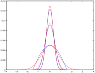
Local descriptors such as SIFT commonly apply a “clamping” procedure to modify a (discretized, spatially-pooled, un-normalized) density of the form (18), by clipping it at a certain threshold , and re-normalizing:
| (28) |
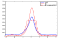
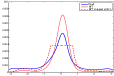
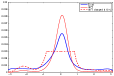
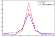
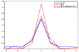
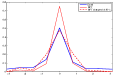
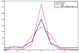
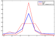
where is typically discretized into bins and is chosen as a percentage of the maximum, for instance . Although clamping has a dramatic effect on performance, with high sensitivity to the choice of threshold, it is seldom explained, other than as a procedure to “reduce the influence of large gradient magnitudes” Lowe (2004).
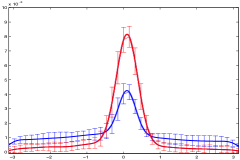
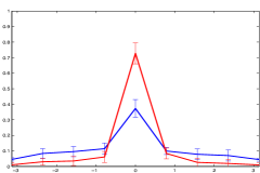
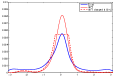
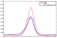
Here, we show empirically that (18) becomes closer to (14) after clamping for certain choices of threshold and sufficiently coarse binning. Fig. 2 shows that, without clamping, (18) is considerably more peaked than (14) and has thinner tails. After clamping, however, the approximation improves, and for coarse binning and threshold between around and the two are very similar.
3.4 Rotation Invariance
Canonization Soatto (2009) is particularly well suited to deal with planar rotation, since it is possible to design co-variant detectors with few isolated extrema. An example is the local maximum of the norm of the gradient along the direction . Invariance to can be achieved by retaining the samples When no consistent (sometimes referred to as “stable”) reference can be found, it means that there is no co-variant functional with isolated extrema with respect to the rotation group, which means that the data is already invariant to rotation.
Note that, again, planar rotations can affect both the training image and the test image . In some cases, a consistent reference (canonical element) is available. For instance, for geo-referenced scenes , and the projection of the gravity vector onto the image plane , , provides a canonical reference unless the two are orthogonal:
| (29) |
4 Deep convolutional architectures
In this section we study the approximation of (12) implemented by convolutional architectures. Starting from (12) for a particular class and a finite number of receptive fields we notice that, since the “true scene” and the nuisances are unknown, we cannot factor the likelihood into a product of , which would correspond to a “bag-of-words” discarding the dependencies in . Convolutional architectures (CNNs) promise to capture such dependencies by hierarchical decomposition into progressively larger receptive fields. Each “layer” is a collection of separator (hidden) variables (nodes) that make lower layers (approximately) conditionally independent.
4.1 Stacking simplifies nuisance marginalization
We show this in several steps. We first argue that managing the group of diffeomorphisms can be accomplished by independently managing small diffeomorphisms in each layer. We use marginalization, but a similar argument can be constructed for max-out or the SA likelihood. Then, we leverage on the local restrictions induced by receptive fields, to deal with occlusion, and argue that such small diffeomorphisms can be reduced locally to a simpler group (affine, similarity, location-scale or even translations, the most common choice in convolutional architectures). Then global marginalization of diffeomorphisms can be accomplished by local marginalization of the reduced group in each layer. The following lemma establishes that global diffeomorphisms can be approximated by the composition of small diffeomorphisms.
Lemma 1.
Let be an orientation-preserving diffeomorphism of a compact subset of the real plane, the identity, and the “size” of . Then for any there exists an and such that and .
Now for two layers, let , with drawn independently from a prior on . Then (or a non-degenerate distribution if are approximated by elements of the reduced group). Then let , or more generally let be defined such that . We then have
| (30) | |||||
| (31) |
where we have also used the fact that . Once the separator variable is reduced to a number of filters, we have
| (32) |
in either case, by extending this construction to layers, we can see that marginalization of each layer can be performed with respect to (conditionally) independent diffeomorphisms that can be chosen to be small per the Lemma above.
Claim 3.
Marginalization of the likelihood with respect to an arbitrary diffeomorphism can be achieved by introducing layers of hidden variables and independently marginalizing small diffeomorphisms at each layer.
The next step is to restrict the marginalization to each receptive field, at which point it can be approximated by a reduced subgroup, or the (linear) generators.
4.2 Hierarchical decomposition of the likelihood
Let
| (33) |
be the marginal likelihood with respect to some prior on and introduce a layer of “separator variables” and group actions , defined such that . This can always be done by choosing ; we will address non-trivial choices later. In either case, forgoing the subscript ,
| (34) |
If and take a finite number and of values (filters) and , then the above reduces to a sum over and ; the conditional likelihoods are the feature maps. If has dimensions and the group actions are taken to be pixel wise translations across the image plane, so that , the feature maps can be represented as a tensor with dimensions . One can repeat the procedure for new separator variables that take possible values, and group actions that take values; the filters must be supported on the entire feature maps (i.e., take values in ) for the sum over to implement the marginalization above
| (35) |
The sum is implemented in convolutional networks by the use of translation invariant filters:
- 1.
-
2.
At the second layer the filter is nonzero for a finite (and small) number of group actions and also satisfies the shift invariant (convolutional) property
The third dimension of the filters is the number of feature maps in the previous layer.
4.3 Approximation of the first layer
Each node in the first layer computes a local representation (5) using parent node(s) as a “scene.” This relates to existing convolutional architectures where nodes compute the response of a rectified linear unit (ReLu) to a filter bank. For simplicity we restrict to the translation group, thus reducing (5) to SIFT, but the arguments apply to similarities.
A ReLu response at to an oriented filter bank with scale and orientation is given by . Let be a Gaussian, centered in with isotropic variance , , . Then is a directional filter with principal orientation and scale . Omitting rectification for now, the response of an image to a filter bank obtained by varying , at each location and for all scales is obtained as
| (36) | |||||
| (37) | |||||
| (38) |
where , the cosine function, has to be rectified for the above to approximate a histogram, which yields SIFT. Unfortunately, in general the latter does not equal for one cannot simply move the maximum inside the integral. However, under conditions on , which are typically satisfied by natural images, this is the case.
Claim 4.
Let be positive, smooth and have a small effective support . I.e., . Let have a sparse and continuous gradient field, so that for every the domain of can be partitioned in three (multiply-connected) regions and the remainder (the complement of their union), where the projection of the gradient in the direction is, respectively, positive, negative, and negligible, and the minimum distance between the regions and . Then, provided that , we have that
| (39) |
4.4 Stacking information
A local hierarchical architecture allows approximating the SA likelihood by reducing nuisance management to local marginalization and max-out of simple group transformations. The SA likelihood is an optimal representation for any query on given data . For instance, for classification, the representation is itself the classifier (discriminant). Thus, if we could compute an optimal classifier, the representation would be the identity; vice-versa, if we could compute the optimal representation, the classifier would be a threshold. In practice, one restricts the family of classifiers – for instance to soft-max, or SVM, or linear – leaving the job of feeding the most informative statistic to the classifier. In a hierarchical architecture, this is the feature maps in the last layer. This is equivalent to neglecting the global dependency on at the last layer. The information loss inherent in this choice is the loss of assuming that are independent (whereas they are only independent conditioned on ).
An optimal representation with restricted complexity , therefore, maximizes the independence of the components of , or equivalently the independence of the components of given . Using those results, one can show that the information content of a representation ((47) in App. A) grows with the number of layers .
5 Discussion
For the likelihood interpretation of a CNN put forward here to make sense, training should be performed generatively, so fixing the class one could sample (hallucinate) future images from the class. However neither the architecture not the training of current CNN incorporate mechanisms to enforce the statistics of natural images.
In this paper we emphasize the role of the task in the representation: If nothing is known about the task, nothing interesting can be said about the representation, and the only optimal one is the trivial one that stores all the data. This is because the task could end up being a query about the value of a particular pixel in a particular image. Nevertheless, there may be many different tasks that share the same representation by virtue of the fact that they share the same nuisances. In fact, the task affects what are nuisance factors, and the nuisance factors affect the design and learning of the representation. For some complex tasks, writing the likelihood function may be prohibitively complex, but some classes of nuisances such as changes of illumination or occlusions, are common to many tasks.
Note that, by definition, a nuisance is not informative. Certain transformations that are nuisances for some tasks may be informative for others (and therefore would not be called nuisances). For instance, viewpoint is a nuisance in object detection tasks, as we want to detect objects regardless of where they are. It is, of course, not a nuisance for navigation, as we must control our pose relative to the surrounding environment. In some cases, nuisance and intrinsic variability can be entangled, as for the case of intra-class deformations and viewpoint-induced deformations in object categorization. Nevertheless, the deformation would be informative if it was known or measured, but since it is not, it must be marginalized.
Our framework does not require nuisances to have the structure of a group. For instance, occlusions do not. Invariance and sensitivity are still defined, as a statistic is invariant if it is constant with respect to variations of the nuisance. What is not defined is the notion of maximal invariance, that requires the orbit structure. However, in our theory maximal invariance is not the focus. Instead, sufficient invariance is.
The literature on the topic of representation is vast and growing. We focus on visual representations, where several have been active. Anselmi et al. (2015) have developed a theory of representation aiming at approximating maximal invariants, which restricts nuisances to (locally) compact groups and therefore do not explicitly handle occlusions. Both frameworks achieve invariance at the expense of discriminative power, whereas in our framework both can be attained at the cost of complexity. Patel et al. (2015), that appeared after earlier drafts of this manuscript were made public, instead of of starting from principles and showing that they lead to a particular kind of computational architecture, instead assume a particular architecture and interpret it probabilistically, similarly to Ver Steeg & Galstyan (2015) that uses total correlation as a proxy of information, which is related to our App. A. However, there the representation is defined absent a task, so the analysis does not account for the role of nuisance factors.
In particular, Anselmi et al. (2015) define a -invariant representation of a (single) image as being selective if for all , i.e., if it is a maximal invariant. But while equivalence to the data up to the action of the nuisance group is critical for reconstruction, it is not necessary for other tasks. Furthermore, for non-group nuisances, such as occlusions, a maximal invariant cannot be constructed. Instead, given a task, we replace maximality with sufficiency for the task, and define at the outset an optimal representation to be a minimal sufficient invariant statistic, or “sufficient invariant,” approximated by the SAL Likelihood. The construction in Anselmi et al. (2015) guarantees maximality for compact groups. Similarly, Sundaramoorthi et al. (2009) have shown that maximal invariants can be constructed even for diffeomorphisms, which are infinite-dimensional and non-compact. In practice, however, occlusions and scaling/quantization break the group structure, and therefore a different approach is needed that relies on sufficiency, not maximality, as we proposed here. To relate our approach to Anselmi et al. (2015), we note that the orbit probability of Def. 4.2 is given by
| (40) |
and is used to induce a probability on , via . On the other hand, we define the minimal sufficient invariant statistic as the marginalized likelihood
| (41) |
where is a (future) image, and is the scene. If we consider the scene to be comprised of a set of images , and the future image , then we see that the OP is a marginalized likelihood where is the Haar measure, and . Thus, substitutions , , yield
| (42) |
for the particular choice of Haar measure and impulsive density . The TP representation can also be understood as a marginalized likelihood, as is the -marginalized likelihood of given when using the uniform prior and an impulsive conditional :
| (43) |
Finally, our treatment of representations is not biologically motivated, in the sense that we simply define optimal representations from first principles, without regards for whether they are implementable with biological hardware. However, we have established connections with both local descriptors and deep neural networks, that were derived using biological inspiration.
Acknowledgments
Work supported by FA9550-15-1-0229, ARO W911NF-15-1-0564, ONR N00014-15-1-2261, and MIUR RBFR12M3AC “Learning meets time.” We are appreciative of discussions with Tomaso Poggio, Lorenzo Rosasco, Stephane Mallat, and Andrea Censi.
References
- Alvarez et al. (1993) Alvarez, L., Guichard, F., Lions, P. L., and Morel, J. M. Axioms and fundamental equations of image processing. Arch. Rational Mechanics, 123, 1993.
- Anselmi et al. (2015) Anselmi, F., Rosasco, L., and Poggio, T. On invariance and selectivity in representation learning. arXiv preprint arXiv:1503.05938, 2015.
- Bahadur (1954) Bahadur, R. R. Sufficiency and statistical decision functions. Annals of Mathematical Statistics, 25(3):423–462, 1954.
- Bengio (2009) Bengio, Y. Learning deep architectures for ai. Foundations and trends® in Machine Learning, 2(1):1–127, 2009.
- Blackwell & Ramamoorthi (1982) Blackwell, D. and Ramamoorthi, R.V. A bayes but not classically sufficient statistic. The Annals of Statistics, 10(3):1025–1026, 1982.
- Boureau et al. (2010) Boureau, Y.-L., Ponce, J., and LeCun, Y. A theoretical analysis of feature pooling in visual recognition. In Proc. of Intl Conf. on Mach. Learning, pp. 111–118, 2010.
- Bouvrie et al. (2009) Bouvrie, J. V., Rosasco, L., and Poggio, T. On invariance in hierarchical models. In NIPS, pp. 162–170, 2009.
- Bruna & Mallat (2011) Bruna, J. and Mallat, S. Classification with scattering operators. In Proc. IEEE Conf. on Comp. Vision and Pattern Recogn., 2011.
- Chatfield et al. (2011) Chatfield, K., Lempitsky, V., Vedaldi, A., and Zisserman, A. The devil is in the details: an evaluation of recent feature encoding methods. 2011.
- Chen & Edelsbrunner (2011) Chen, C. and Edelsbrunner, H. Diffusion runs low on persistence fast. In ICCV, pp. 423–430, 2011.
- Cover & Thomas (1991) Cover, T. M. and Thomas, J. A. Elements of Information Theory. Wiley, 1991.
- Creutzig et al. (2009) Creutzig, F., Globerson, A., and Tishby, N. Past-future information bottleneck in dynamical systems. Phys. Rev. Lett. E, 79(4):19251–19255, 2009.
- DeGroot (1989) DeGroot, M. H. Probability and statistics. Addison-Wesley, 1989.
- Dong & Soatto (2014) Dong, J. and Soatto, S. Machine Learning for Computer Vision, chapter Visual Correspondence, the Lambert-Ambient Shape Space and the Systematic Design of Feature Descriptors. R. Cipolla, S. Battiato, G.-M. Farinella (Eds), Springer Verlag, 2014.
- Dong & Soatto (2015) Dong, J. and Soatto, S. Domain size pooling in local descriptors: Dsp-sift. In Proc. IEEE Conf. on Comp. Vision and Pattern Recogn., 2015.
- Fraser & Naderi (2007) Fraser, D. and Naderi, A. Minimal sufficient statistics emerge from the observed likelihood function. International Journal of Statistical Science, 6:55–61, 2007.
- Gong et al. (2014) Gong, Y., Wang, L., Guo, R., and Lazebnik, S. Multi-scale orderless pooling of deep convolutional activation features. arXiv preprint arXiv:1403.1840, 2014.
- Grenander (1993) Grenander, U. General Pattern Theory. Oxford University Press, 1993.
- Hinkley (1979) Hinkley, D. Predictive likelihood. The Annals of Statistics, pp. 718–728, 1979.
- Huang & Mumford (1999) Huang, J. and Mumford, D. Statistics of natural images and models. In Proc. CVPR, pp. 541–547, 1999.
- Kirchner (2015) Kirchner, M. R. Automatic thresholding of SIFT descriptors. Technical Report, 2015.
- LeCun (2012) LeCun, Y. Learning invariant feature hierarchies. In ECCV, pp. 496–505, 2012.
- Lowe (2004) Lowe, D. G. Distinctive image features from scale-invariant keypoints. IJCV, 2(60):91–110, 2004.
- Mikolajczyk et al. (2004) Mikolajczyk, K., Tuytelaars, T., Schmid, C., Zisserman, A., Matas, J., Schaffalitzky, F., Kadir, T., and Gool, L. Van. A comparison of affine region detectors. IJCV, 1(60):63–86, 2004.
- Morel & Yu (2011) Morel, J. M. and Yu, G. Is sift scale invariant? Inverse Problems and Imaging, 5(1):115–136, 2011.
- Patel et al. (2015) Patel, A., Nguyen, T., and Baraniuk, R. A probabilistic theory of deep learning. arXiv preprint arXiv:1504.00641, 2015.
- Pawitan (2001) Pawitan, Y. In all likelihood: Statistical modeling and inference using likelihood. Oxford, 2001.
- Ranzato et al. (2007) Ranzato, M., Huang, F. J., Boureau, Y.-L., and LeCun, Y. Unsupervised learning of invariant feature hierarchies with applications to object recognition. In CVPR, pp. 1–8, 2007.
- Serre et al. (2007) Serre, T., Oliva, A., and Poggio, T. A feedforward architecture accounts for rapid categorization. Proceedings of the National Academy of Sciences, 104(15):6424–6429, 2007.
- Shao (1998) Shao, J. Mathematical Statistics. Springer Verlag, 1998.
- Simonyan et al. (2014) Simonyan, K., Vedaldi, A., and Zisserman, A. Learning local feature descriptors using convex optimisation. IEEE Trans. Pattern Anal. Mach. Intell., 2(4), 2014.
- Soatto (2009) Soatto, S. Actionable information in vision. In Proc. of the Intl. Conf. on Comp. Vision, October 2009.
- Sundaramoorthi et al. (2009) Sundaramoorthi, G., Petersen, P., Varadarajan, V. S., and Soatto, S. On the set of images modulo viewpoint and contrast changes. In Proc. IEEE Conf. on Comp. Vision and Pattern Recogn., June 2009.
- Susskind et al. (2011) Susskind, J., Memisevic, R., Hinton, G. E., and Pollefeys, M. Modeling the joint density of two images under a variety of transformations. In Proc. IEEE Conf. on Comp. Vision and Pattern Recogn., pp. 2793–2800, 2011.
- Tishby et al. (2000) Tishby, N., Pereira, F. C., and Bialek, W. The information bottleneck method. In Proc. of the Allerton Conf., 2000.
- Ver Steeg & Galstyan (2015) Ver Steeg, G. and Galstyan, A. Maximally informative hierarchical representations of high-dimensional data. in depth, 13:14, 2015.
Appendix A Quantifying the information content of a representation
In general we do not know the likelihood, but we have a collection of samples , each generated with some nuisance , which we can use to infer, or “learn” an approximation of the SAL likelihood Fraser & Naderi (2007).
| (44) | |||||
| (45) | |||||
| (46) |
Depending on modeling choices made, including the number of samples , the sampling mechanism, and the priors for local marginalization, the resulting representation will be “lossy” compared to the data. Next we quantify such a loss.
A.1 Informative content of a representation
The scene is in general infinite-dimensional. Thus, the informative content of the data cannot be directly quantified by mutual information . In fact, and therefore, no matter how many (finite) data we have, is not defined. Similarly, is undefined and therefore mutual information cannot be used directly to measure the informative content of a representation, or to infer the most informative statistic.
The notion of Actionable Information Soatto (2009) as where is a maximal -invariant, can be used to bypass the computation of : Writing formally
| (47) |
we see that, if we were given the scene , we could generate the data , under the action of some nuisance , up to the residual modeling uncertainty, which is assumed white and zero-mean (lest the mean and correlations of the residual can be included in the model). Similarly, we can generate a maximal invariant up to a residual with constant entropy; therefore, the statistic which maximizes is the one that maximizes the first term in (47), . This formal argument allows defining the most informative statistic as the one that maximizes Actionable Information, , bypassing the computation of the entropy of the “scene” . Note that the task still influences the information content of a representation, by defining what are the nuisances , which in turn affect the computation of actionable information.
An alternative approach is to measure the informative content of a representation bypassing consideration of the scene is described next.
Definition 1 (Informative Content of a Representation).
The information a statistic of conveys on is the information it conveys on a task (e.g., a question on the scene ), regardless of nuisances :
| (48) |
If the task is reconstruction (or prediction) , where past data and future data are generated by the same scene , then the definition above relates to the past-future mutual information Creutzig et al. (2009) except for the role of the nuisance . The following claim shows that an ideal representation, as previously defined in terms of minimal sufficient invariant statistic, maximizes information.
Claim 5.
Let past data and future data , used to accomplish a task , be generated by the same scene . Then the representation maximizes the informative content of a representation.
The next claim relates a representation to Actionable Information.
Claim 6.
If maximizes Actionable Information, it also maximizes the informative content of a representation.
Note that maximizing Actionable Information is a stronger condition than maximizing the information content of a representation. Since Actionable Information concerns maximal invariance, sufficiency is automatically implied, and the only role the task plays is the definition of the nuisance group . This is limiting, since we want to handle nuisances that do not have the structure of a group, and therefore Definition 48 affords more flexibility than Soatto (2009).
The next two claims characterize the maximal properties of the profile likelihood. We first recall that the marginalized likelihood is invariant only if marginalization is done with respect to the base (Haar) measure, and in general it is not a maximal invariant, as one can show easily with a counter-example (e.g., a uniform density). On the other hand, the profile likelihood is by construction invariant regardless of the distribution on , but is also – in general – not maximal. However, it is maximal under general conditions on the likelihood. To see this, consider to be given; for a free variable , it can be written as a map : . For a fixed , is a function of . If is constant along (the level curves are straight lines), then in general for all does not imply . Indeed, can be arbitrarily different from . Even if is non-degenerate (non-constant along certain directions), but presents symmetries, it is possible for different to yield the same for all . However, under generic conditions for all implies . Now consider to be given; for a free variable the map can be written using a function such that . Note that is, by construction, invariant to . Also note that, following the same argument as above, the invariant is not maximal, for it is possible for for all and yet and are not equivalent (equal up to a constant : ). However, if the function is generic, then the invariant is maximal. In fact, let , so that . If we now have for all , then we can conclude, based on the argument above, that . Since and are fixed, and the equality is for all , we can conclude that is independent of . That allows us to conclude the following.
Claim 7 (Maximality of the profile likelihood).
If the density is generic with respect to , then is a maximal -invariant.
Since we do not have control on the function , which is instead in general constructed from data, it is legitimate to ask what happens when the generic condition above is not satisfied. Fortunately, distributions that yield non-maximal invariants can be ruled out as uninformative at the outset:
Claim 8 (Non-maximality and non-informativeness).
If is such that, for any we have for all , then is uninformative.
This follows from the definition of information, for any statistic .
As we have pointed out before, what matters is not that the invariant be maximal, but that it be sufficient. As anticipated in Rem. 1, we can achieve invariance with no sacrifice of discriminative power, albeit at the cost of complexity.
Appendix B Proofs
Theorem 1
Proof.
Pick any , define and and apply the factorization lemma with . ∎
Theorem 2
Proof.
We denote with the normalized gradient of , and similarly for ; maps it to polar coordinates and , where
The conditional density of given takes the polar form
| (49) |
Defining to be the -th component of , (49) can be expanded as
| (50) |
and the exponent is
| (51) |
We are now interested in the marginal of (50) with respect to , i.e.,
| (52) |
where we can isolate the factor that does not depend on ,
| (53) |
The bracketed term is the integral on the interval of a Gaussian density with mean and variance ; it can be rewritten, using the change of variable , as which can be integrated by parts to yield
and therefore
| (54) |
which, once written explicitly in terms of and , yields (14)-(15). ∎
Claim 5
Proof.
Since is sufficient for , and it factorizes into , then is sufficient of for . By the factorization theorem (Theorem 3.1 of Pawitan (2001)), there exist functions and such that , i.e., the likelihood depends on the data only through the function . This latter function is what is more commonly known as the sufficient statistic, which in particular has the property that . However, if is sufficient for , it is also sufficient for future data generated from . Formally,
| (55) |
which shows that minimizes the uncertainty of for any since the right-hand-side is -invariant. The right-hand side above is the predictive likelihood Hinkley (1979), which must therefore be proportional to for some and the same , also by the factorization theorem. ∎
Claim 4
Proof.
(Sketch) The integral in (38) can be split into 3 components, one of which omitted, leaving the positive component integrated on , the negative component on . If the distance between these two is greater than , however, the components are disjoint, so for each and , only the the positive or the negative component are non-zero, and since and are both positive, and the sign is constant, rectification inside or outside the integral is equivalent. When there is an error in the approximation, that can be bounded as a function of , the minimum distance and the maximum gradient component. ∎
A more general kernel could be considered, with a parameter that controls the decay, or width, of the kernel, . For instance, , with the default value being . An alternative is to define to be an angular Gaussian with dispersion parameter , which is constrained to be positive and therefore does not need rectification. Although the angular Gaussian is quite different from the cosine kernel for , it approximates it as decreases (Fig. 4).
A corollary of the above is that the visible layer of a CNN computes the SAL Likelihood of the first hidden layer.
The interpretation of SIFT as a likelihood function given the test image can be confusing, as ordinarily it is interpreted as a “feature vector” associated to the training image , and compared with other feature vectors using the Euclidean distance. In a likelihood interpretation, is used to compute the likelihood function, and is used to evaluate it. So, there is no descriptor built for . The same interpretational difference applies to convolutional architectures. If interpreted as a likelihood, which would require generative learning, one would compute the likelihood of different hypotheses given the test data. Instead, currently the test data is fed to the network just as training data were, thus generating features maps, that are then compared (discriminatively) by a classifier.