Output Feedback Stabilization of Switched Linear Systems with Limited Information

Abstract

We propose an encoding and control strategy for the stabilization of switched systems with limited information, supposing that the controller is given for each mode. Only the quantized output and the active mode of the plant at each sampling time are transmitted to the controller. Due to switching, the active mode of the plant may be different from that of the controller in the closed-loop system. Hence if switching occurs, the quantizer must recalculate a bounded set containing the estimation error for quantization at the next sampling time. We establish the global asymptotic stability under a slow-switching assumption on dwell time and average dwell time. To this end, we construct multiple discrete-time Lyapunov functions with respect to the state and the size of the bounded set.

I Introduction

Digital devices such as samplers, quantizers, and communication channels play an indispensable role in low-cost, intelligent control systems. This has motivated researchers to study control problems with limited information due to sampling and quantization, as surveyed in [1, 2, 3]. On the other hand, many systems encountered in practice have switching among several modes of operation. The stabilization problem of switched systems has also been studied extensively; see the book [4], the survey [5, 6], and many references therein.

Both sampling/quantization and switching are discrete-time dynamics and often appear in control systems simultaneously. The authors of [7, 8, 9, 10] have studied quantized control for Markov jump discrete-time systems. In [11], the stabilization of Markov jump systems with uniformly sampled mode information is investigated. However, for switched systems with deterministic switching signals, most works deal with sampling/quantization and switching separately. Based on the result in [12], our previous work [13] has developed an output encoding strategy for switched system under an average dwell-time condition [14] but have not considered sampling.

The following difficulty arises from partial knowledge of the switching signal due to sampling: Switching can lead to the mismatch of the active modes between the plant and the controller. Accordingly, we need to prepare for another encoding strategy in case switching occurs. For the quantization at the next sampling time, an encoding strategy after a switch happens must include the estimation of intersample information, e.g., the state behavior in the sampling interval, from the transmitted data.

For switched systems with sampling and quantization, state feedback stabilization has been studied under a slow-switching assumption in [15, 16]. By contrast, we assume that the information on the quantized output and the active mode of the plant is transmitted to the controller at each sampling time. The objective of this paper is to develop an encoding and control strategy achieving global asymptotic stabilization for given state feedback gains. The detection of switching within each sampling interval requires a dwell-time assumption. On the other hand, we also use an average dwell-time assumption for the convergence of the state to the origin.

Our proposed method can be seen as the extension of [15] from state feedback to output feedback and also that of [17] from non-switched systems to switched systems. A data-rate bound derived from our result is that from [17] maximized over all the subsystems.

We organize this paper as follows. In Section II, first we show the switched linear system and the information structure we consider. After placing some basic assumptions, we state the main result. Section III is devoted to the so-called “zooming-out” stage, whose objective is to measure the output adequately. In Section IV, we provide the encoding and control strategy that makes the state converges to the origin, and obtain a bound on the set in which the estimation error can reach when a switch occurs. In Section V, we show that the Lyapunov stability is achieved. and Section VI contains a numerical example. Finally we conclude this paper in Section VII.

Notation:  Let $\mathbb{Z}_{+}$ be the set of non-negative integers. For $t\in\mathbb{R}$, $\lfloor t\rfloor$ is the largest integer not greater than $t$.

Let $\lambda_{\min}(P)$ and $\lambda_{\max}(P)$ denote the smallest and the largest eigenvalue of $P\in\mathbb{R}^{\sf n\times n}$. Let $M^{\top}$ denote the transpose of $M\in\mathbb{R}^{\sf m\times n}$.

The Euclidean norm of $v\in\mathbb{R}^{\sf n}$ is denoted by $|v|=(v^{*}v)^{1/2}$. The Euclidean induced norm of $M\in\mathbb{R}^{\sf m\times n}$ is defined by $\|M\|=\sup\{|Mv|:~{}v\in\mathbb{R}^{\sf n},~{}|v|=1\}$. For $v=[v_{1}~{}\!\dotsb~{}\!v_{\sf n}]^{\top}\in\mathbb{R}^{\sf n}$, its maximum norm is $|v|_{\infty}=\max\{|v_{1}|,\dots,|v_{\sf n}|\}$, and the corresponding induced norm of $M\in\mathbb{R}^{\sf m\times n}$ is given by $\|M\|_{\infty}=\sup\{|Mv|_{\infty}:~{}v\in\mathbb{R}^{\sf n},~{}|v|_{\infty}=1\}$.

II Output Stabilization of Switched Systems with Limited Information

II-A Switched Systems and Information Structure

Consider the switched linear system

$$\dot{x}=A_{\sigma}x+B_{\sigma}u,\quad y=C_{\sigma}x,$$ (1)

where $x(t)\in\mathbb{R}^{\sf{n}}$ is the state, $u(t)\in\mathbb{R}^{\sf{m}}$ is the control input, and $y(t)\in\mathbb{R}^{\sf{p}}$ is the output. For a finite index set $\mathcal{P}$, the function $\sigma:~{}[0,\infty)\to\mathcal{P}$ is right-continuous and piecewise constant. We call $\sigma$ switching signal and the discontinuities of $\sigma$ switching times. Let $N_{\sigma}(t,s)$ stand for their number in the interval $(s,t]$.

To generate the control input $u$, we can use the following information on the output $y$ and the switching signal $\sigma$:

Sampling:  Let $\tau_{s}>0$ be the sampling period. The output $y$ and the switching signal $\sigma$ are measured only at sampling times $k\tau_{s}$ $(k\in\mathbb{Z}_{+})$.

Quantization:  Pick an odd positive number $N$. The measured output $y(k\tau_{s})$ is encoded by an integer in $\{1,2\dots,N^{\sf{p}}\}$. This encoded output and the sampled switching signal $\sigma(k\tau_{s})$ are transmitted to the controller.

For the Lyapunov stability in Section V, we take $N$ to be odd. Fig. 1 shows the closed loop we consider.

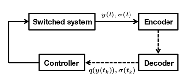
Figure 1: Sampled-data switched system with quantized output feedback

II-B Main Result

Our first assumption is the stabilizability and observability of each subsystem.

Assumption II.1

For every $p\in\mathcal{P}$, $(A_{p},B_{p})$ is stabiliable and $(C_{p},A_{p})$ is observable. We choose $K_{p}\in\mathbb{R}^{\sf m\times n}$ so that $A_{p}+B_{p}K_{p}$ is Hurwitz. For all $A_{p}$. the sampling time $\tau_{s}$ is not pathological.

The non-pathological sampling time implies that $(C_{p},e^{A_{p}\tau_{s}})$ is observable in the discrete-time sense, which is used for state reconstruction.

Next we assume that the switching signal $\sigma$ has the following slow-switching properties:

Assumption II.2

Dwell time:  Every interval between two switches is not smaller than the sampling period $\tau_{s}$. That is, $N_{\sigma}(t,s)\leq 1$ if $t-s\leq\tau_{s}$.

Average dwell time [14]:  There exist $\tau_{a}>0$ and $N_{0}\in\mathbb{N}$ such that

$$N_{\sigma}(t,s)\leq N_{0}+\frac{t-s}{\tau_{a}}$$ (2)

for all $t>s\geq 0$.

Switching signals in Assumption II.2 are called hybrid dwell-time signals [18, 15]. The assumption on dwell time is necessary for the detection of a switch between sampling times, while that on average dwell time is used in the proof that the state converges to the origin.

Furthermore, we extend the quantization assumption for systems with a single mode in [17] to switched systems.

Assumption II.3

Let $\eta_{p}$ be the smallest natural number such that $W_{p}$ defined by

$$W_{p}=\begin{bmatrix}C_{p}\\ C_{p}e^{A_{p}\tau_{s}}\\ \vdots\\ C_{p}e^{A_{p}(\eta_{p}-1)\tau_{s}}\end{bmatrix}$$ (3)

has full column rank. Let $W_{p}^{\dagger}$ be a left inverse of $W_{p}$. Then

$$\|e^{A_{p}\eta_{p}\tau_{s}}W_{p}^{\dagger}\|_{\infty}\cdot\max_{0\leq k\leq\eta_{p}-1}\left\|C_{p}e^{A_{p}k\tau_{s}}\right\|_{\infty}<N$$ (4)

for all $p\in\mathcal{P}$.

Assumption II.3 gives a lower bound on the available data rate implicitly, and (4) is the data-rate bound from [17] maximized over the individual modes. This assumption is used for finer quantization when a switch does not occur. Note that as $\tau_{s}$ becomes small, $e^{A_{p}\eta_{p}\tau_{s}}$ and $C_{p}e^{A_{p}k\tau_{s}}$ converge to $I$ and $C_{p}$ respectively, but that $W_{p}$ does not have full column rank in general if $\tau_{s}=0$. Therefore the left side of (4) may not decrease as $\tau_{s}$ tends to zero.

If $C_{p}=I$, then $W_{p}=I$ and $\eta_{p}=1$. Hence (4) is consistent to the data rate assumption in the state feedback case [15].

The main result shows that global asymptotic stabilization is possible if the average dwell time is sufficiently large.

Theorem II.4

Consider the switched system (1), and let Assumptions II.1, II.2, and II.3 hold. If the average dwell time $\tau_{a}$ in (2) is larger than a certain value, then there exists an output encoding that achieves the following stability for every $x(0)\in\mathbb{R}^{\sf n}$ and every $\sigma(0)\in\mathcal{P}$:

Convergence to the origin: 

$$\lim_{t\to\infty}x(t)=0.$$ (5)

Lyapunov stability:  To every $\varepsilon>0$, there corresponds $\delta>0$ such that if $|x(0)|<\delta$, then $|x(t)|<\varepsilon$ for $t\geq 0$.

A constructive proof of Theorem II.4 is given in the next sections. We obtain a sufficient condition (42) on $\tau_{a}$ in the proof. As in [17, 13, 15], we show the convergence to the origin by dividing the proof into the “zooming-out” stage and the “zooming-in” stage.

III Zooming-out Stage

The objective of the “zooming-out” stage is to generate an upper bound on the estimation error of the state. We have to obtain such a bound by using the quantized output and the switching signal at each sampling time.

Define $\eta$ by

$$\eta=\max_{p\in\mathcal{P}}\eta_{p}.$$ (6)

At this stage, we set the control input $u=0$. Assume that the average dwell time $\tau_{a}$ satisfies

$$\tau_{a}>\eta\tau_{s}.$$ (7)

Pick $\mu_{0}>0$ and $\chi>0$, and define

$$\mu_{n}=e^{(1+\chi)\max_{p\in\mathcal{P}}\|A_{p}\|_{\infty}n\tau_{s}}\mu_{0}$$ (8)

for $n\in\mathbb{Z}_{+}$. We construct the encoding function $Q_{n}$ by

$$Q_{n}(y)=\begin{cases}0&\quad\text{if~{}~{}}y(n\tau_{s})\in\{y\in\mathbb{R}^{\sf p}:~{}|y|_{\infty}\leq\mu_{n}\}\\ 1&\quad\text{otherwise}.\end{cases}$$

The following theorem is used for the reconstruction of the state:

Theorem III.1

If the average dwell time $\tau_{a}$ in (2) satisfies (7), then there exists an integer $n_{0}\geq 0$ such that

$$Q_{n}(y)=0$$ (9)

$$\sigma(n\tau_{s})=\sigma(n_{0}\tau_{s})=:p$$ (10)

for $n=n_{0},n_{0}+1,\dots,n_{0}+\eta_{p}-1$. Such $n_{0}$ satisfies $n_{0}\leq n_{1}$, where $n_{1}$ depends on $N_{0}$ and $\tau_{a}$ in (2) but not on $\sigma$ itself.

To prove Theorem III.1, we use the following property of average dwell time:

Lemma III.2 ([13])

Fix an initial time $t_{0}\geq 0$. Suppose that $\sigma$ satisfies (2). Let $\tau_{0}\in(0,\tau_{a})$, and choose an integer $m$ such that

$$m>\frac{\tau_{a}}{\tau_{a}-\tau_{0}}\left(N_{0}-\frac{\tau_{0}}{\tau_{a}}\right).$$ (11)

There exists $T\in[t_{0},t_{0}+(m-1)\tau_{0}]$ such that $N_{\sigma}(T+\tau_{0},T)=0$.

Proof:

The growth rate of $\mu_{n}$ in (8) is larger than that of $|y|_{\infty}$ for arbitrary switching. Hence there is an integer $\bar{n}_{0}$ such that $|y|_{\infty}\leq\mu_{n}$ for all $n\geq\bar{n}_{0}$, which leads to (9).

Let $m$ be an integer satisfying (11) with $\eta\tau_{s}$ in place of $\tau_{0}$. Since $\tau_{a}>\eta\tau_{s}$, Lemma III.2 shows that $N_{\sigma}(T+\eta\tau_{s},T)=0$ for some $T\in[\bar{n}_{0}\tau_{s},(\bar{n}_{0}+(m-1)\eta)\tau_{s}]$. The interval $(T,T+\eta\tau_{s}]$ contains $\eta$ sampling times. Thus we have an integer $n_{0}\in[\bar{n}_{0},\bar{n}_{0}+(m-1)\eta]$ satisfying (9) and (10) for $n=n_{0},n_{0}+1,\dots,n_{0}+\eta_{p}-1$, and $n_{0}\leq n_{1}:=\bar{n}_{0}+(m-1)\eta$. ∎

In conjunction with the dwell-time assumption, (10) shows that the active mode of the plant does not change in $[n_{0}\tau_{s},(n_{0}+\eta_{p}-1)\tau_{s}]$. We can therefore reconstruct $x(n_{0}\tau_{s})$ by using $W_{p}$ in (3) and the output at $t=n_{0}\tau_{s},\dots,(n_{0}+\eta_{p}-1)\tau_{s}$:

$$x(n_{0}\tau_{s})=W_{p}^{\dagger}\begin{bmatrix}y(n_{0}\tau_{s})\\ \vdots\\ y((n_{0}+\eta_{p}-1)\tau_{s})\end{bmatrix}.$$ (12)

The rest of the procedure is the same as in the non-switched case [17]. Combining (9) and (12), we obtain

$$|x(n_{0}\tau_{s})|_{\infty}\leq\|W_{p}^{\dagger}\|_{\infty}\cdot\mu_{n_{0}+\eta_{p}-1}=:E_{n_{0}}.$$ (13)

It follows that

$$|x((n_{0}+\eta_{p})\tau_{s})|_{\infty}\leq e^{\max_{p\in\mathcal{P}}\|A_{p}\|_{\infty}\tau_{s}} \left\|e^{A_{p}(\eta_{p}-1)\tau_{s}}\right\|_{\infty}E_{n_{0}}=:E_{n_{0}+\eta_{p}}.$$ (14)

Define the estimated state $\xi$ at $t=(n_{0}+\eta_{p})\tau_{s}$ by

$$\xi((n_{0}+\eta_{p})\tau_{s})=0.$$ (15)

Then the error $e=x-\xi$ satisfies $|e((n_{0}+\eta_{p})\tau_{s})|_{\infty}\leq E_{n_{0}+\eta}.$ This completes the “zooming-out” stage.

IV Zooming-in Stage

Here we construct an encoding and control strategy for the convergence of the state to the origin. Since the size $E_{k}$ of the quantization region increases after a switch occurs, the term “zooming-in” may be misleading. However, in order to contrast the “zooming-out” phase in the previous section, we call the stage in this section the “zooming-in” stage as in [12, 19].

Let $t_{0}=k_{0}\tau_{s}\geq 0$ be the initial time of the zooming-in stage or the time at which the upper bound $E_{k}$ of the estimation error is updated. Let $\xi$ and $e$ be the estimated state and the estimation error $x-\xi$, respectively. Assume that $\sigma(k_{0}\tau_{s})=p$ and $|e(k_{0}\tau_{s})|_{\infty}\leq E_{k_{0}}$.

IV-A Basic encoding and control method

If no switch happens, then we can use the encoding and control method for systems with a single mode in [17]. However, after a switch occurs, a modified upper bound on the estimation error is needed for the next quantized measurement. We shall obtain the upper bound in Section IV. C. 1). In this subsection, assuming that the state estimate $\xi(k_{0})$ and the error bound $E_{k_{0}}$ are derived, we briefly state the encoding and control method because it will be needed in the sequel.

Let $\sigma(k_{0}\tau_{s})=p$. If no switch occurs in $(t_{k_{0}},t_{k_{0}+\eta_{p}\tau_{s}}]$, we set $k=\eta_{p}$, and otherwise we define $k$ by the minimum integer in the interval $[1,\eta_{p}]$ such that $\sigma((k_{0}+k-1)\tau_{s})\not=\sigma((k_{0}+k)\tau_{s})$. We generate the state estimate $\xi$ and the output estimate $\hat{y}$ by

$$\dot{\xi}=(A_{p}+B_{p}K_{p})\xi,\quad\hat{y}=C_{p}\xi$$ (16)

for $t\in[k_{0}\tau_{s},(k_{0}+k)\tau_{s})$, and set the control input

$$u=K_{p}\xi.$$ (17)

Since $\dot{x}=A_{p}x+B_{p}K_{p}\xi,$ it follows that $e=x-\xi$ satisfies

$$\dot{e}=A_{p}e.$$ (18)

If $l=0,\dots,k-1$, then

$$|y((k_{0}+l)\tau_{s})-\hat{y}((k_{0}+l)\tau_{s})|_{\infty} \leq\left\|C_{p}e^{A_{p}l\tau_{s}}\right\|_{\infty}E_{k_{0}}.$$

For $l=0,\dots,k-1$, divide the hypercube

$$\left\{y\in\mathbb{R}^{\sf p}:~{}|y-\hat{y}((k_{0}+l)\tau_{s})|_{\infty}\leq\left\|C_{p}e^{A_{p}l\tau_{s}}\right\|_{\infty}E_{k_{0}}\right\}$$ (19)

into $N^{\sf p}$ equal boxes and assign a number in $\{1,\dots,N^{\sf p}\}$ to each divided box by a certain one-to-one mapping. The encoder sends to the decoder the number $Q_{k_{0}+l}$ of the divided box containing $y((k_{0}+l)\tau_{s})$, and then the decoder generates $q_{k_{0}+l}$ equal to the center of the box with number $Q_{k_{0}+l}$. If $y((k_{0}+l)\tau_{s})$ lies on the boundary on several boxes, then we can choose any one of them.

IV-B Non-switched case

The calculation of an upper bound $E_{k}$ on the estimation error is dependent of whether a switch occurs in an interval with length $\eta_{p}\tau_{s}$. Let us first study the case without switching in the interval $(k_{0}\tau_{s},(k_{0}+\eta_{p})\tau_{s}]$, i.e., the case $\sigma(k_{0}\tau_{s})=\dots=\sigma((k_{0}+\eta_{p})\tau_{s})=:p$.

IV-B1 Calculation of an error bound

An upper bound $E_{k_{0}+\eta_{p}}$ on $|e((k_{0}+\eta_{p})\tau_{s})|_{\infty}$ can be obtained in the same way as in [17]. We therefore omit the details of the calculation here.

Define

$$\theta_{p}=\frac{\|e^{A_{p}\eta_{p}\tau_{s}}W_{p}^{\dagger}\|_{\infty}\cdot\max_{0\leq k\leq\eta_{p}-1}\left\|C_{p}e^{A_{p}k\tau_{s}}\right\|_{\infty}}{N}.$$ (20)

From the result in [17], if we appropriately determine $\xi$ at $t=(k_{0}+\eta_{p})\tau_{s}$ from the transmitted data $q_{k_{0}},\dots,q_{k_{0}+\eta_{p}-1}$, then we obtain $|e(t_{0}+\eta_{p}\tau_{s})|_{\infty}\leq E_{k_{0}+\eta_{p}}$, where $E_{k_{0}+\eta_{p}}$ is defined by

$$E_{k_{0}+\eta_{p}}=\theta_{p}E_{k_{0}}.$$ (21)

Note that $\theta_{p}<1$ for every $p\in\mathcal{P}$ by (4).

IV-B2 Decrease rate of multiple Lyapunov functions

Here we construct a discrete-time Lyapunov function $V_{p}$ of mode $p$ with respect to $x(k\tau_{s})$ and $E_{k}$. The calculation below is similar to that in the state feedback case [15], but we sketch it for completeness.

For simplicity of notation, we write $V_{p}(k)$ instead of $V_{p}(x(k\tau_{s}),E_{k})$. We obtain an upper bound of $V_{p}(k_{0}+\eta_{p})$ using $V_{p}(k_{0})$.

First we obtain $x((k_{0}+\eta_{p})\tau_{s})$ from $x(k_{0}\tau_{s})$ and $e(k_{0}\tau_{s})$. Since

$$\dot{x}=A_{p}x+B_{p}K_{p}\xi=(A_{p}+B_{p}K_{p})x-B_{p}K_{p}e$$ (22)

for $t\in[k_{0}\tau_{s},(k_{0}+\eta_{p})\tau_{s})$, it follows from (18) that

$$x((k_{0}+\eta_{p})\tau_{s})=\bar{A}_{p}x(k_{0}\tau_{s})+\bar{B}_{p}e(k_{0}\tau_{s}),$$ (23)

where $\bar{A}_{p}$ and $\bar{B}_{p}$ are defined by

$$\bar{A}_{p} =e^{(A_{p}+B_{p}K_{p})\eta_{p}\tau_{s}}$$

$$\bar{B}_{p} =\int^{\eta_{p}\tau_{s}}_{0}e^{(A_{p}+B_{p}K_{p})(\eta_{p}\tau_{s}-t)}B_{p}K_{p}e^{A_{p}t}dt.$$

Recall that $\bar{A}_{p}$ is Hurwitz by Assumption II.3. To every positive definite matrix $Q_{p}$, there correponds a positive definite matrice $P_{p}$ such that

$$\bar{A}_{p}^{\top}P_{p}\bar{A}_{p}-P_{p}=-Q_{p}.$$ (24)

Fix $\rho_{p}>0$ for each $p\in\mathcal{P}$. Similarly to [15], define the Lyapunov function $V_{p}$ by

$$V_{p}(k)=V_{p}(x(k\tau_{s}),E_{k})=x(k\tau_{s})^{\top}P_{p}x(k\tau_{s})+\rho_{p}E_{k}^{2}.$$ (25)

Pick $\kappa_{p}>1$. A simple computation gives

$$x((k_{0}+\eta_{p})\tau_{s})^{\top}P_{p}x((k_{0}+\eta_{p})\tau_{s})-x(k_{0}\tau_{s})^{\top}P_{p}x(k_{0}\tau_{s})$$

$$\quad\leq-\lambda_{\min}(Q_{p})|x(k_{0}\tau_{s})|^{2}+2\|\bar{A}_{p}^{\top}P_{p}\bar{B}_{p}\|\cdot|x(k_{0}\tau_{s})|\cdot|e(k_{0}\tau_{s})|+\|\bar{B}_{p}^{\top}P_{p}\bar{B}_{p}\|\cdot|e(k_{0}\tau_{s})|^{2}$$

$$\quad\leq-\frac{1}{\kappa_{p}}\lambda_{\min}(Q_{p})|x(k_{0}\tau_{s})|^{2}-\frac{\kappa_{p}-1}{\kappa_{p}}\left(\sqrt{\lambda_{\min}(Q_{p})}\cdot|x(k_{0}\tau_{s})|-\frac{\kappa_{p}}{\kappa_{p}-1}\frac{\|\bar{A}_{p}^{\top}P_{p}\bar{B}_{p}\|}{\sqrt{\lambda_{\min}(Q_{p})}}|e(k_{0}\tau_{s})|\right)^{2}$$

$$\qquad\qquad+\left(\frac{\kappa_{p}}{\kappa_{p}-1}\frac{\|\bar{A}_{p}^{\top}P_{p}\bar{B}_{p}\|^{2}}{\lambda_{\min}(Q_{p})}+\|\bar{B}_{p}^{\top}P_{p}\bar{B}_{p}\|\right)|e(k_{0}\tau_{s})|^{2}$$

$$\quad\leq-\alpha_{p}|x(k_{0}\tau_{s})|^{2}+\beta_{p}E_{k_{0}}^{2},$$ (26)

where $\alpha_{p}$ and $\beta_{p}$ are defined by

$$\alpha_{p} =\frac{1}{\kappa_{p}}\lambda_{\min}(Q_{p})$$

$$\beta_{p} ={\sf n}\left(\frac{\kappa_{p}}{\kappa_{p}-1}\frac{\|\bar{A}_{p}^{\top}P_{p}\bar{B}_{p}\|^{2}}{\lambda_{\min}(Q_{p})}+\|\bar{B}_{p}^{\top}P_{p}\bar{B}_{p}\|\right).$$

Combining (21) with (26), as in [15, Lemma 1], we obtain

$$V_{p}(k_{0}+\eta_{p}) \leq\left(1-\frac{\alpha_{p}}{\lambda_{\max}(P_{p})}\right)x(k_{0}\tau_{s})^{\top}P_{p}x(k_{0}\tau_{s})+\left(\frac{\beta_{p}}{\rho_{p}}+\theta_{p}^{2}\right)\rho_{p}E_{k_{0}}^{2}.$$

Since $\theta_{p}<1$, we can choose $\rho_{p}$ so that

$$\rho_{p}>\frac{\beta_{p}}{1-\theta_{p}^{2}}.$$ (27)

Then defining

$$\nu_{p}:=\max\left\{1-\frac{\alpha_{p}}{\lambda_{\max}(P_{p})},~{}~{}\frac{\beta_{p}}{\rho_{p}}+\theta_{p}^{2}\right\}<1,$$ (28)

we finally obtain

$$V_{p}(k_{0}+\eta_{p})\leq\nu_{p}V_{p}(k_{0}).$$ (29)

Note that $\nu_{p}$ depends on $\kappa_{p}>1$ and $\rho_{p}$ with (27). We can use these parameters to make the encoding and control strategy less conservative, i.e., to allow smaller average dwell time.

IV-C Switched case

Next we study the case in which a switch occurs in the interval $(k_{0}\tau_{s},(k_{0}+\eta_{p})\tau_{s}]$. Suppose that $k\in\mathbb{N}$, with $k\leq\eta_{p}$, for which the first switching time $T$ after $k_{0}\tau_{s}$ satisfies $T\in((k_{0}+k-1)\tau_{s},(k_{0}+k)\tau_{s}].$ That is, $\sigma(k_{0}\tau_{s})=\dots=\sigma((k_{0}+k-1)\tau_{s})=:p$ and $\sigma((k_{0}+k-1)\tau_{s})\not=\sigma((k_{0}+k)\tau_{s})=:q$. In this case, the estimated state $\xi$ and the controller input $u$ in the interval $[k_{0}\tau_{s},(k_{0}+k)\tau_{s}]$ are given by (16) and (17), respectively. Note that the switching information is not transmitted instantly. However, the controller can detect the switch at the next sampling time. This is because the dwell-time condition in Assumption II.2 implies that at most one switch occurs between sampling time.

IV-C1 Calculation of an error bound

Our first objective here is to obtain an upper bound $E_{k_{0}+k}$ of $|e((k_{0}+k)\tau_{s})|_{\infty}$ from the information $\xi(k_{0}\tau_{s})$ and $E_{k_{0}}$ available to the quantizer.

Lemma IV.1

Define $H_{p,q}$, $\bar{\delta}_{p,q}(k)$, and $\bar{\gamma}_{p,q}^{\prime}(k)$ by

$$H_{p,q}=(A_{q}-A_{p})+(B_{q}-B_{p})K_{p}$$ (30)

$$\bar{\delta}_{p,q}(k)=\max_{0\leq\tau\leq\tau_{s}}\left\|\int^{\tau_{s}}_{\tau}e^{A_{q}(\tau_{s}-t)}H_{p,q}e^{(A_{p}+B_{p}K_{p})(t+(k-1)\tau_{s})}dt\right\|_{\infty}$$

$$\bar{\gamma}_{p,q}^{\prime}(k)=\max_{0\leq\tau\leq\tau_{s}}\left\|e^{A_{q}(\tau_{s}-\tau)}e^{A_{p}((k-1)\tau_{s}+\tau)}\right\|_{\infty}.$$

Then we obtain the following upper bound of $|e(t_{0}+k\tau_{s})|_{\infty}$:

$$|e((k_{0}+k)\tau_{s})|_{\infty}\leq\bar{\delta}_{p,q}(k)|\xi(k_{0}\tau_{s})|_{\infty}+\bar{\gamma}_{p,q}^{\prime}(k)E_{k_{0}}=:E_{k_{0}+k}.$$ (31)

Proof:

Since $e$ is determined by (18) before the switching time $T$, it follows that

$$e(T)=e^{A_{p}(T-k_{0}\tau_{s})}e(k_{0}\tau_{s}).$$

Let us consider the error behavior for $t>T$. The mode of the plant changes from $p$ to $q$ after $T$, while that of the controller is still $p$. We therefore have

$$\dot{x}=A_{q}x+B_{q}K_{p}\xi,$$ (32)

and it follows that $e$ satisfies

$$\dot{e}=A_{q}e+H_{p,q}\xi$$ (33)

for $t>T$, where $H_{p,q}$ is defined by (30).

As regards $\xi$, (16) gives

$$\xi(t)=e^{(A_{p}+B_{p}K_{p})(t-k_{0}\tau_{s})}\xi(k_{0}\tau_{s})$$ (34)

for $t\in[k_{0}\tau_{s},(k_{0}+k)\tau_{s}]$. Substituting this into (33), we obtain

$$e((k_{0}+k)\tau_{s})=e^{A_{q}(\tau_{s}-\tau)}e^{A_{p}((k-1)\tau_{s}+\tau)}e(k_{0}\tau_{s})+\int^{\tau_{s}}_{\tau}e^{A_{q}(\tau_{s}-t)}H_{p,q}e^{(A_{p}+B_{p}K_{p})(t+(k-1)\tau_{s})}dt\cdot\xi(k_{0}\tau_{s}),$$

where $\tau=T-(k_{0}+k-1)\tau_{s}$ and $0<\tau\leq\tau_{s}$. Thus we obtain (31). ∎

Remark IV.2

(1) The propose method discards the quantized measurements $q_{k_{0}},\dots,q_{k-1}$. If we use these data, then a better $E_{k}$ can be obtained, in particular, in the case when a switch occurs in the last sampling interval $((k_{0}+\eta_{p}-1)\tau_{s},(k_{0}+\eta_{p})\tau_{s}]$.

Here we briefly explain how to obtain the error bound in the switched case by using the quantized measurements $q_{k_{0}},\dots,q_{k-1}$. For simplicity, let us assume that the switching time $T$ is in the last sampling interval, i.e., $T\in((k_{0}+\eta_{p}-1)\tau_{s},(k_{0}+\eta_{p})\tau_{s}]$, and let and $\sigma((k_{0}+\eta_{p}-1)\tau_{s})=p$ and $\sigma((k_{0}+\eta_{p})\tau_{s})=q\not=p$. In this case, we can construct the state estimate $\zeta_{0}$ for $x(k_{0}\tau_{s})$ by using the measurements $q_{k_{0}},\dots,q_{k_{0}+\eta_{p}-1}$. We assume that $|\zeta_{0}-x(k_{0}\tau_{s})|_{\infty}\leq E_{\zeta}$.

Similarly to $\xi$ in (16), we define the dynamics of $\zeta$ by

$$\dot{\zeta}=A_{p}\zeta+B_{p}u,\qquad\zeta(k_{0}\tau_{s})=\zeta_{0}.$$

Define $e_{\zeta}=x-\zeta$. Recalling that $u=K_{p}\xi$, we can write the dynamics of $e_{\zeta}$ after a switch as

$$\dot{e}_{\zeta}=A_{q}e_{\zeta}+(A_{q}-A_{p})\zeta+(B_{q}-B_{p})K_{p}\xi,$$

and hence

$$e_{\zeta}((k_{0}+\eta_{p})\tau_{s})=F_{1}(T)e_{\zeta}(k_{0}\tau_{s})+F_{2}(T)\zeta_{0}+F_{3}(T)\xi(k_{0}\tau_{s})$$

for some continuous functions $F_{1}$, $F_{2}$, and $F_{3}$. Therefore if we define the new state estimate $\xi((k_{0}+\eta_{p})\tau_{s})$ by

$$\xi((k_{0}+\eta_{p})\tau_{s}):=\zeta((k_{0}+\eta_{p})\tau_{s}),$$

then the error bound $E_{k_{0}+\eta_{p}}$ is given by

$$E_{k_{0}+\eta_{p}}=\max_{T\in I_{0}}\|F_{1}(T)\|_{\infty}\cdot E_{\zeta}+\max_{T\in I_{0}}\|F_{2}(T)\|_{\infty}\cdot|\zeta_{0}|_{\infty}+\max_{T\in I_{0}}\|F_{3}(T)\|_{\infty}\cdot|\xi(k_{0}\tau_{s})|_{\infty},$$

where $I_{0}:=[(k_{0}+\eta_{p}-1)\tau_{s},(k_{0}+\eta_{p})\tau_{s}]$.

(2) For simplicity, we use (34) for the estimated state at $t=(k_{0}+k)\tau_{s}$. However, this estimate makes the corresponding bound $E_{k_{0}+k}$ be larger if the switch occurs just after the sampling time. To avoid this conservatism, two auxiliary time variables can be used as in [15, Section 4.2].

IV-C2 Increase rate of multiple Lyapunov functions

Let us next find an upper bound of $V_{q}(k_{0}+k)$ described by $V_{p}(k_{0})$. To this end, we need upper bounds on $|x((k_{0}+k)\tau_{s})|$ and $E_{k_{0}+k}$ by using $|x(k_{0}\tau_{s})|$ and $E_{k_{0}}$.

Lemma IV.3

Define $\bar{\delta}_{p,q}$ and $\bar{\gamma}_{p,q}^{\prime}$ as in Lemma IV.1 and also $\bar{\gamma}_{p,q}$ by $\bar{\gamma}_{p,q}(k)=\bar{\delta}_{p,q}(k)+\bar{\gamma}_{p,q}^{\prime}(k)$. Then we have

$$E_{k_{0}+k}\leq\bar{\delta}_{p,q}(k)|x(k_{0}\tau_{s})|+\bar{\gamma}_{p,q}(k)E_{k_{0}}.$$ (35)

Proof:

This follows from the definition (31) of $E_{k_{0}+k}$ and

$$|\xi(k_{0}\tau_{s})|_{\infty}\leq|x(k_{0}\tau_{s})|_{\infty}+|e(k_{0}\tau_{s})|_{\infty}\leq|x(k_{0}\tau_{s})|+E_{k_{0}}.$$

∎

Remark IV.4

Note that $E_{k_{0}+k}$ must be determined from the available data $\xi(k_{0}\tau_{s})$ and $E_{k_{0}}$. In contrast, since the variables of the Lyapunov function $V_{q}$ are $x(k_{0}\tau_{s})$ and $E_{k_{0}}$, we need an upper bound on $E_{k_{0}+k}$ described by $x(k_{0}\tau_{s})$ and $E_{k_{0}}$. If we use $\xi$ as a variable of the Lyapunov functions as in [15], then the conservatism in Lemma IV.3 can be avoided. Instead of that, however, (26) becomes conservative.

Now we obtain an upper bound of $|x((k_{0}+k)\tau_{s})|$.

Lemma IV.5

Define $\bar{\alpha}_{p,q}(k)$ and $\bar{\beta}_{p,q}(k)$ by

$$\bar{\alpha}_{p,q}(k) =\max_{0\leq\tau\leq\tau_{s}}\left\|e^{A_{q}(\tau_{s}-\tau)}e^{(A_{p}+B_{p}K_{p})\tau(k)}+\int^{\tau_{s}}_{\tau}e^{A_{q}(\tau_{s}-t)}B_{q}K_{p}e^{(A_{p}+B_{p}K_{p})(t+(k-1)\tau_{s})}dt\right\|.$$

$$\bar{\beta}_{p,q}(k) =\sqrt{\sf n}\max_{0\leq\tau\leq\tau_{s}}\biggr{\|}e^{A_{q}(\tau_{s}-\tau)}\int^{\tau(k)}_{0}e^{(A_{p}+B_{p}K_{p})(\tau(k)-t)}B_{p}K_{p}e^{A_{p}t}dt$$

$$\qquad\qquad\qquad\qquad\qquad-\int^{\tau_{s}}_{\tau}e^{A_{q}(\tau_{s}-t)}B_{q}K_{p}e^{(A_{p}+B_{p}K_{p})(t+(k-1)\tau_{s})}dt\biggr{\|}.$$

Then we derive

$$|x((k_{0}+k)\tau_{s})|\leq\bar{\alpha}_{p,q}(k)|x(k_{0}\tau_{s})|+\bar{\beta}_{p,q}(k)E_{k_{0}}.$$ (36)

Proof:

Recall that $x$ and $e$ satisfy (22) and (18) before the switching time $T$. Defining $\tau(k)=T-k_{0}\tau_{s},$ we have

$$x(T)=e^{(A_{p}+B_{p}K_{p})\tau(k)}x(k_{0}\tau_{s})+\int^{\tau(k)}_{0}e^{(A_{p}+B_{p}K_{p})(\tau(k)-t)}B_{p}K_{p}e^{A_{p}t}dt\cdot e(k_{0}\tau_{s}).$$ (37)

On the other hand, since $x$ satisfies (32) after the switching time $T$, it follows from (34) that

$$x(( k_{0}+k)\tau_{s})=e^{A_{q}(\tau_{s}-\tau)}x(T)+\int^{\tau_{s}}_{\tau}e^{A_{q}(\tau_{s}-t)}B_{q}K_{p}e^{(A_{p}+B_{p}K_{p})(t+(k-1)\tau_{s})}dt\cdot(x(k_{0}\tau_{s})-e(k_{0}\tau_{s})),$$ (38)

where $\tau=T-(k_{0}+k-1)\tau_{s}$ and $0<\tau\leq\tau_{s}$. Substituting (37) into (38), we derive the desired result (36). ∎

Similarly to [15, Lemma 2], (35) and (36) show that

$$V_{q}(k_{0}+k)\leq\frac{2(\lambda_{\max}(P_{q})\bar{\alpha}_{p,q}^{2}+\rho_{q}\bar{\delta}_{p,q}^{2})}{\lambda_{\min}(P_{p})}x(k_{0}\tau_{s})^{\top}P_{q}x(k_{0}\tau_{s})+\frac{2(\lambda_{\max}(P_{q})\bar{\beta}_{p,q}^{2}+\rho_{q}\bar{\gamma}_{p,q}^{2})}{\rho_{p}}\rho_{p}E_{k_{0}}^{2}.$$ (39)

Thus if the switching time $T\in((k_{0}+k-1)\tau_{s},(k_{0}+k)\tau_{s}]$, then the bound (39) gives

$$V_{q}(k_{0}+k)\leq\bar{\nu}_{p,q}(k)V_{p}(k_{0}),$$ (40)

where $\bar{\nu}_{p,q}(k)$ is defined by

$$\bar{\nu}_{p,q}(k) =\max\biggl{\{}\frac{2(\lambda_{\max}(P_{q})\bar{\alpha}_{p,q}(k)^{2}+\rho_{q}\bar{\delta}_{p,q}(k)^{2})}{\lambda_{\min}(P_{p})},~{}~{}\frac{2(\lambda_{\max}(P_{q})\bar{\beta}_{p,q}(k)^{2}+\rho_{q}\bar{\gamma}_{p,q}(k)^{2})}{\rho_{p}}\biggr{\}}.$$

IV-D Convergence to the origin

Finally, we combine the average dwell-time property with the bounds (29) and (40) on the Lyapunov functions.

Lemma IV.6

Define $\nu$ and $\bar{\nu}$ by

$$\nu=\max_{p\in\mathcal{P}}\nu_{p},\quad\bar{\nu}=\max_{p\not=q}\max_{1\leq k\leq\eta_{p}}\bar{\nu}_{p,q}(k).$$ (41)

If the average dwell time $\tau_{a}$ satisfies

$$\tau_{a}>\left(1+\frac{\log\bar{\nu}}{\log(1/\nu)}\right)\eta\tau_{s},$$ (42)

where $\eta$ is defined by (6), then the state converges to the origin, that is, (5) holds.

Proof:

If we have no switches, then convergence to the origin directly follows from stabilizability of each mode. Hence we assume that switches occur. Fix an integer $M>k_{0}$. Let the switching times in the interval $(k_{0}\tau_{s},M\tau_{s}]$ be $T_{1},\dots,T_{r}$. Suppose that $T_{i}\in((k_{i}-1)\tau_{s},k_{i}\tau_{s}]$. By Assumption II.2, $k_{i-1}\leq k_{i}-1$ for $i=1,\dots,r$.

Define $\psi_{i}$ and $\ell_{i}$ by

$$\psi_{i}=\left\lfloor\frac{k_{i}-k_{i-1}-1}{\eta_{\sigma(k_{i-1}\tau_{s})}}\right\rfloor,\quad\ell_{i}=k_{i-1}+\psi_{i}\eta_{\sigma(k_{i-1}\tau_{s})}$$

for $i=1,\dots,r$. Then $\sigma(k_{i}\tau_{s})\not=\sigma(\ell_{i}\tau_{s})$ and $\sigma(\ell_{i}\tau_{s})=\sigma(k_{i-1}\tau_{s})$. Moreover, since

$$\frac{k-n+1}{n}\leq\left\lfloor\frac{k}{n}\right\rfloor\leq\frac{k}{n}$$ (43)

for $k,n\in\mathbb{N}$, it follows that $1\leq k_{i}-\ell_{i}\leq\eta_{\sigma(k_{i-1}\tau_{s})}$. This means that we have $\psi_{i}$ intervals with length $\eta_{\sigma(k_{i-1}\tau_{s})}\tau_{s}$ in which no switch occurs and that the switched case in Section IV. C starts at $t=\ell_{i}\tau_{s}$. We therefore obtain

$$V_{\sigma(k_{i}\tau_{s})}(k_{i})\leq\bar{\nu}V_{\sigma(\ell_{i}\tau_{s})}(\ell_{i})\leq\bar{\nu}\nu^{\psi_{i}}V_{\sigma(k_{i-1}\tau_{s})}(k_{i-1})$$ (44)

for $i=1,\dots,r$.

Now we investigate the Lyapunov functions after the last switching time $T_{r}$. As before, define

$$\psi_{r+1}=\left\lfloor\frac{M-k_{r}}{\eta_{\sigma(k_{r}\tau_{s})}}\right\rfloor,\quad\ell_{r+1}=k_{r}+\psi_{r+1}\eta_{\sigma(k_{r}\tau_{s})}.$$

A discussion similar to the above shows that

$$V_{\sigma(M\tau_{s})}(M)\leq\hat{\nu}\nu^{\psi_{r+1}}V_{\sigma(k_{r}\tau_{s})}(k_{r})~{}\text{for some $\hat{\nu}>0$.}$$ (45)

Let us combine the Lyapunov functions before and after the last switching time $T_{r}$. Define $\psi$ by

$$\psi=\sum_{i=1}^{r+1}\psi_{i}.$$ (46)

Then (44) and (45) shows that

$$V_{\sigma(M\tau_{s})}(M)\leq\hat{\nu}\bar{\nu}^{r}\nu^{\psi}V_{\sigma(k_{0}\tau_{s})}(k_{0}).$$ (47)

We see from (43) that $\psi$ in (46) satisfies

$$\psi \geq\frac{M-k_{0}+1}{\eta}-(r+1),$$ (48)

where $\eta$ is defined by (6). Substituting (48) into (47), we obtain

$$V_{\sigma(M\tau_{s})}(M)\leq\hat{\nu}\nu^{1/\eta-1}\cdot\bar{\nu}^{r}\nu^{(M-k_{0})/\eta-r}V_{\sigma(k_{0}\tau_{s})}(k_{0}).$$ (49)

Suppose that $r=N_{\sigma}(M\tau_{s},k_{0}\tau_{s})$ satisfies the average dwell-time condition (2). Then

$$\bar{\nu}^{r}\nu^{(M-k_{0})/\eta-r}\leq\bar{\nu}^{N_{0}}\nu^{-N_{0}}\cdot\left(\bar{\nu}^{\tau_{s}/\tau_{a}}\nu^{1/\eta-\tau_{s}/\tau_{a}}\right)^{M-k_{0}}.$$

Thus if $\tau_{a}$ satisfies $\bar{\nu}^{\tau_{s}/\tau_{a}}\nu^{1/\eta-\tau_{s}/\tau_{a}}<1$, i.e., (42) holds, then we have $\lim_{M\to\infty}V_{\sigma(M\tau_{s})}(M)=0.$

From the convergence of $V_{\sigma}$, we easily obtain the desired result (5). The definition (25) of $V_{\sigma(M\tau_{s})}$ shows that $|x(M\tau_{s})|$ and $|e(M\tau_{s})|_{\infty}$ are bounded by the constant multiplication of $\sqrt{V_{\sigma(M\tau_{s})}(M)}$, and so is $|\xi(M\tau_{s})|$. Hence

$$\lim_{M\to\infty}x(M\tau_{s})=\lim_{M\to\infty}\xi(M\tau_{s})=0.$$

Since the behavior of $x$ between sampling times is given by (22) and (32), it follows that

$$|x(M\tau_{s}+\tau)|\leq L_{1}|x(M\tau_{s})|+L_{2}|\xi(M\tau_{s})|\qquad(0<\tau<\tau_{s})$$

for some $L_{1},L_{2}\geq 0$. Thus the state converges to the origin not only at sampling times but also in sampling intervals. ∎

Remark IV.7

(1) To avoid a trivial result, we assume that $\bar{\nu}\geq 1$. Then (42) implies (7), which is the assumption on $\tau_{a}$ at the “zooming-out” stage.

(2) From (42), we see the relationship between switching and data rate. If we increase $N$ in (4), then $\gamma_{p}$ defined by (20) decreases and hence so do $\nu_{p}$ in (28) and $\nu$ in (41). This leads to a decrease in $\tau_{a}$.

(3) Piecewise linear Lyapunov functions are also applicable if an induced norm of $e^{(A_{p}+B_{p}K_{p})\eta_{p}\tau_{s}}$ is less than one for every $p\in\mathcal{P}$. For example, $\|e^{(A_{p}+B_{p}K_{p})\eta_{p}\tau_{s}}\|_{\infty}<1$ allows us to construct $V_{p}=|x|_{\infty}+\rho_{p}E$ and $V_{p}=|\xi|_{\infty}+\rho_{p}E$. The advantage is that the computation of their upper bounds are simpler than in the quadratic case. Such Lyapunov functions may provide less conservative results.

V Lyapnov Stability

The point here is to find an upper bound on the finish time of the “zooming-out” stage and an upper bound on the time after which the state with non-zero control input remains in $\varepsilon$-neighborhood of the origin at the “zooming-in” stage. Such bounds are dependent on $\tau_{a}$ and $N_{0}$ in (2), but not on a switching signal itself. The former follows from Lemma III.2 and the latter proceeds along the same lines as in Sec. 5.5 of [15].

Let us first investigate the final time of the “zooming-out” stage.

Assume that the average dwell time condition (42) holds, and let $m$ be an interger satisfying (11) with $\eta\tau_{s}$ in place of $\tau_{0}$. Lemma III.2 with $t_{0}=0$ shows that for such $m$, there exists an integer $n_{0}\in[0,(m-1)\eta]$ such that

$$\sigma(t)=\sigma(n_{0}\tau_{s})=:p$$

for $t\in[n_{0}\tau_{s},(n_{0}+\eta-1)\tau_{s}]$. Moreover, if $\delta$ satisfies

$$C_{\max}e^{\max_{p\in\mathcal{P}}\|A_{p}\|_{\infty}(m\eta-1)\tau_{s}}\delta<\mu_{0},$$

where we define $C_{\max}=\max_{p\in\mathcal{P}}\|C_{p}\|_{\infty}$, then $|y(n\tau_{s})|_{\infty}\leq\mu_{0}\leq\mu_{n}$, and hence $Q_{n}(y)=0$ for all $n=0,1,\dots,(m-1)\eta$. For $E_{n_{0}}$ defined by (13), (12) shows that

$$|x(n_{0}\tau_{s})|_{\infty}\leq E_{n_{0}}\leq\max_{p\in\mathcal{P}}\|W^{\dagger}_{p}\|_{\infty}\cdot\mu_{m\eta-1}=:\bar{E}_{0}.$$

This leads to

$$|x((n_{0}+\eta_{p})\tau_{s})|_{\infty} \leq e^{\max_{p\in\mathcal{P}}\|A_{p}\|_{\infty}\tau_{s}}\left\|e^{A_{p}(\eta_{p}-1)\tau_{s}}\right\|_{\infty}E_{n_{0}}(=:E_{n_{0}+\eta_{p}})$$

$$\leq e^{\max_{p\in\mathcal{P}}\|A_{p}\|_{\infty}\tau_{s}}\cdot\max_{p\in\mathcal{P}}\left\|e^{A_{p}(\eta_{p}-1)\tau_{s}}\right\|_{\infty}\cdot\bar{E}_{0}=:\bar{E}.$$

for all $p\in\mathcal{P}$ and $n_{0}\in[0,(m-1)\eta]$. This bound $\bar{E}$ is independent on a switching signal itself and satisfies $E_{n_{0}+\eta_{p}}\leq\bar{E}$. Also the final time $(n_{0}+\eta_{p})\tau_{s}$ of the “zooming-out” stage is smaller than $m\eta$, which does depend on $N_{0}$ and $\tau_{a}$, but not on a switching signal itself.

Next we study the time after which the state with non-zero control input remains in $\varepsilon$-neighborhood of the origin at the “zooming-in” stage.

The discussion above shows that the initial time $t_{0}:=k_{0}\tau_{s}:=(n_{0}+\eta_{p})\tau_{s}$ of the “zooming-in” stage satisfies $k_{0}\leq m$ and that $|x(k_{0}\tau_{s})|_{\infty}\leq E_{k_{0}}\leq\bar{E}$. Define $\Lambda_{\max}$ by

$$\Lambda_{\max}=\max_{p\in\mathcal{P}}({\sf n}\lambda_{\max}(P_{p})+\rho_{p}).$$

Since $e(k_{0}\tau_{s})=x(k_{0}\tau_{s})$, it follows that the Lyapunov function in (25) satisfies $V_{\sigma(k_{0})\tau_{s}}\leq\Lambda_{\max}\bar{E}^{2}.$ Thus we see from (47) that, for all $M\geq k_{0}$

$$V_{\sigma(M\tau_{s})}(M)\leq\hat{\nu}\bar{\nu}^{N_{\sigma}(M\tau_{s},k_{0}\tau_{s})}\nu^{\psi}\Lambda_{\max}\bar{E}^{2}.$$ (50)

In conjunction with (42), this shows that, for every $\varepsilon>0$, there exists $M_{0}\geq 0$ such that $V_{\sigma(M\tau_{s})}(M)<\varepsilon$ for $M\geq M_{0}$. Hence for every $\varepsilon>0$, there also exists $T_{0}\geq 0$ such that

$$|x(t)|_{\infty}<\varepsilon\qquad(t\geq T_{0}).$$ (51)

Notice that (50) implies that $M_{0}$ depends on $N_{0}$, $\tau_{a}$, and $\varepsilon$ but not on a switching signal itself, and so does $T_{0}$.

If we obtain

$$|x(t)|_{\infty}<\varepsilon\qquad(t\leq T_{0}),$$ (52)

then combining (51) and (52) completes the proof for Lyapunov stability.

We see from (14), (19), and (21) that if $\delta$ satisfies

$$C_{\max}e^{\max_{p\in\mathcal{P}}\|A_{p}\|_{\infty}T_{0}}\delta \leq\frac{1}{\sf p}\min_{p\in\mathcal{P}}\min_{0\leq k\leq\eta_{p}-1}\|C_{p}e^{A_{p}k\tau_{s}}\|_{\infty}\cdot(\min_{p\in\mathcal{P}}\theta_{p})^{\lfloor T_{0}/\min_{p\in\mathcal{P}}\eta_{p}\rfloor}$$

$$\qquad\times\min_{p\in\mathcal{P}}\left(\left\|e^{A_{p}(\eta_{p}-1)\tau_{s}}\right\|_{\infty}\cdot\|W^{\dagger}_{p}\|_{\infty}\right)\mu_{0},$$

then the quantized output $q_{k}$ is zero for $kT_{s}\leq T_{0}$. This means that $\xi(t)=u(t)=0$ for $t\leq T_{0}$. Therefore if $\delta$ additinally satisfies

$$e^{\max_{p\in\mathcal{P}}\|A_{p}\|_{\infty}T_{0}}\delta<\varepsilon,$$

then we have (52).

In Fig. 2, we illustrate the state trajectory for the Lyapunov stability.

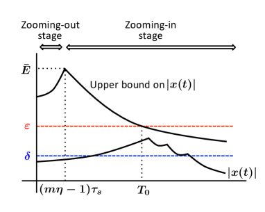
Figure 2: The state trajectory for the Lyapunov stability

VI Numerical Example

Consider a continuous-time switched system (1) with the following two modes:

$$A_{1}=\begin{bmatrix}0&-1\\ -1&-2\end{bmatrix},\quad B_{1}=\begin{bmatrix}1\\ -1\end{bmatrix},\quad C_{1}=\begin{bmatrix}1&1\end{bmatrix}$$

$$A_{2}=\begin{bmatrix}1&2\\ -2&-1\end{bmatrix},\quad B_{2}=\begin{bmatrix}-2\\ 1\end{bmatrix},\quad C_{2}=\begin{bmatrix}1&-1\end{bmatrix}.$$

The feedback gains of each mode are $K_{1}=[-1~{}~{}2]$ and $K_{2}=[1~{}~{}-1]$. Note that $A_{1}+B_{1}K_{2}$ and $A_{2}+B_{2}K_{1}$ have an unstable pole $2.2361$ and $4$, respectively. The sampling period $\tau_{s}$ and the partition number $N$ of the quantizer are $\tau_{s}=0.5$ and $N=11$.

We took $Q_{1}$ and $Q_{2}$ in (24) and the parameters of $\nu_{1}$ and $\nu_{2}$ in (28) as follows: $Q_{1}=Q_{2}=I$, $\kappa_{1}=1.124$, $\kappa_{2}=1.09$, $\rho_{1}=47$, and $\rho_{2}=80$. These were chosen by trial and error. We see from (42) that if $\tau_{a}>5.55$, our encoding and control strategy achieves the global asymptotic stabilization.

A time response in the interval $[0,20]$ was calculated for $x(0)=[-3~{}~{}3]^{\top}$, $\mu_{0}=0.1$, and $\chi=1$. The switching signal was chosen so that the dwell time $\tau_{d}=2.6$ and (2) holds with $N_{0}=1$ and the average dwell time $\tau_{a}=5.8$. Fig. 3 shows the Euclidean norm of the state $x$ and the state estimate $\xi$. In this simulation, the “zooming-out” stage finished at $t=1$ but we observe that the system was not controlled until $t=2$. The reason is that the state estimate is zero at the end of “zooming-out” stage; see (15). This leads to no control input in the initial period of “zooming-in” stage as in the “zooming-out” stage.

If the state of the plant is accessible, i.e., $C_{1}=C_{2}=I$, then we see from [15, Assumption 3] that if the number of symbols in the quantizer is not smaller than $3^{2}+1=10$, then the encoding and control strategy in [15] stabilizes the plant. On the other hand, the counterpart in the output feedback case from (4) is $5+1=6$. Hence in this example, if we consider only stabilization of systems with sufficiently large average-dwell time property, then the use of the output with lower dimension than the dimension of the state has the advantage in terms of data rate.

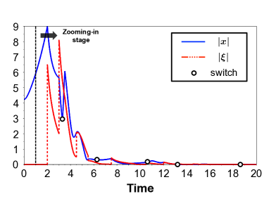
Figure 3: The Euclidean norm of the state $x$ and the estimated state $\xi$

VII Concluding Remarks

We have studied the problem of stabilizing a switched linear system with limited information: the quantized output and active mode at each sampling time. We have supposed that the controller is given and have examined the intersample behavior of the estimation error for the encoding strategy after the detection of switching. Using multiple discrete-time Lyapunov functions, we have achieved global asymptotic stabilization under the hybrid dwell-time assumption. The data-rate bound used here is the maximum among the bounds of the individual subsystems that are from the earlier work.

References

- [1] G. N. Nair, F. Fagnani, S. Zampieri, and R. J. Evans, “Feedback control under data rate constraints: An overview,” Proc. IEEE, vol. 95, pp. 108–137, 2007.
- [2] J. P. Hespanha, P. Naghshtabrizi, and Y. Xu, “A survey of rrecent results in networked control systems,” Proc. IEEE, vol. 95, pp. 138–162, 2007.
- [3] H. Ishii and K. Tsumura, “Data rate limitations in feedback control over network,” IEICE Trans. Fundamentals, vol. E95-A, pp. 680–690, 2012.
- [4] D. Liberzon, Switching in Systems and Control. Birkhäuser, Boston, 2003.
- [5] R. Shorten, F. Wirth, O. Mason, K. Wulff, and C. King, “Stability criteria for switched and hybrid systems,” SIAM Review, vol. 49, pp. 545–592, 2007.
- [6] H. Lin and P. J. Antsaklis, “Stability and stabilizability of switched linear systems: a survey of recent results,” IEEE Trans. Automat. Control, vol. 54, pp. 308–322, 2009.
- [7] G. N. Nair, S. Dey, and R. J. Evans, “Infinmum data rates for stabilising markov jump linear systems,” in Proc. 42nd IEEE CDC, 2003.
- [8] Q. Ling and H. Lin, “Necessary and sufficient bit rate conditions to stabilize quantized markov jump lineaer systems,” in Proc. ACC 2010, 2010.
- [9] N. Xiao, L. Xie, and M. Fu, “Stabilization of Markov jump linear systems using quantized state feedback,” Automatica, vol. 46, pp. 1696–1702, 2010.
- [10] Q. Xu, C. Zhang, and G. E. Dullerud, “Stabilization of Markovian jump linear systems with log-quantized feedback,” J. Dynamic Systems, Meas, Control, vol. 136, pp. 1–10 (031 919), 2013.
- [11] A. Cetinkaya and T. Hayakawa, “Feedback control of switched stochastic systems using uniformly sampled mode information,” in ACC 2012, 2012.
- [12] D. Liberzon, “Hybrid feedback stabilization of systems with quantized signals,” Automatica, vol. 39, pp. 1543–1554, 2003.
- [13] M. Wakaiki and Y. Yamamoto, “Quantized output feedback stabilization of switched linear systems,” in Proc. MTNS 2014, 2014.
- [14] J. P. Hespanha and A. S. Morse, “Stability of swithched systems with average dwell-time,” in Proc. 38th IEEE CDC, 1999.
- [15] D. Liberzon, “Finite data-rate feedback stabilization of switched and hybrid linear systems,” Automatica, vol. 50, pp. 409–420, 2014.
- [16] M. Wakaiki and Y. Yamamoto, “Quantized feedback stabilization of sampled-data switched linear systems,” in Proc. 19th World Congress of IFAC, 2014.
- [17] D. Liberzon, “On stabilization of linear systems with limited information,” IEEE Trans. Automat. Control, vol. 48, pp. 304–307, 2003.
- [18] L. Vu and D. Liberzon, “Supervisory control of uncertain linear time-varying systems,” IEEE Trans. Automat. Control, vol. 56, pp. 27–42, 2011.
- [19] R. W. Brockett and D. Liberzon, “Quantized feedback stabilization of linear systems,” IEEE Trans. Automat. Control, vol. 45, pp. 1279–1289, 2000.