Central density cusps in the Lemaître-Tolman solutions

Abstract

The character of the central density profile in the Lemaître-Tolman (LT) solutions plays a fundamental role in their application as cosmological models. This same character is studied here for these solutions used to model complete gravitational collapse. A necessary condition for the development of a black hole (not even locally naked singularities) is developed. This condition allows a finite (invariantly) defined range in central density cusps. If one demands no density cusps in the initial conditions, then this work shows that the LT solutions never produce even locally naked singularities.

I Introduction

Certainly the most widely used exact solution of the Einstein equations is that of spherically symmetric inhomogeneous dust, often referred to as the Lemaître-Tolman (LT) (and sometimes as the Lemaître-Tolman-Bondi (LTB)) model. One can find very detailed discussions of these solutions in some modern texts pk . There is a very extensive application of these models in cosmology Bolejko , and their use in the study of nakedly singular gravitational collapse goes back at least 35 years es . For general discussions of these models see pk , the earlier text Krasinski , and gp . There are many more recent discussions. The evolution of radial profiles (which is not of primary concern here) see sus1 , and for various considerations of gravitational entropy (which are of interest here) see sus2 .

One of the most interesting applications of the LT models in cosmology is the reproduction of observables of the $\Lambda$CDM model without $\Lambda$. The LT models that do this have central density cusps ce . Naturally, such behavior elicits two points of view: the density profiles are unphysical vfw , and the density profiles are just fine ok .

The purpose of the present communication is to examine the role that the central density profiles play in gravitational collapse. Whereas the usual treatment of the LT models involves coordinates $(r,\theta,\phi,t)$, where $r$ is some radial coordinate, $\theta$ and $\phi$ are the usual angular coordinates, and $t$ is the proper time along the geodesic streamlines of the fluid, it is necessary for the present discussion (as explained below) to switch to coordinates $(m,\theta,\phi,t)$, where $m$ is the effective gravitation mass hm . For clarity, the solution is developed from first principles in the next section (see also pk ).

II The LT model

Starting with Einstein’s equations notation

$$G_{\alpha\beta}=8\pi T_{\alpha\beta}=8\pi\rho\;u_{\alpha}u_{\beta},$$ (1)

where the $u^{\alpha}$ are tangent to the generators of the geodesic flow, we consider only positive definite energy densities $\rho>0$, and use comoving synchronous coordinates so that

$$ds^{2}=e^{\alpha(m,t)}dm^{2}+R^{2}(m,t)d\Omega^{2}-dt^{2}$$ (2)

where $d\Omega^{2}$ is the metric of a unit two-sphere, which we write in the usual form $d\theta^{2}+\sin^{2}(\theta)d\phi^{2}$, and we assume the existence of an origin defined by $R(0,t)=0$ (and all $t$ derivatives of $R(0,t)=0$). The generators of the flow are $u^{\alpha}=\delta^{\alpha}_{t}$ and the radial normals are $n^{\alpha}=\pm e^{-\alpha/2}\delta^{\alpha}_{m}$ so that $-u^{\alpha}u_{\alpha}=n^{\alpha}n_{\alpha}=1$ and $u^{\alpha}n_{\alpha}=0$. From

$$G_{\alpha\beta}u^{\alpha}n^{\beta}=0$$ (3)

we find

$$e^{\alpha}=\frac{(R^{{}^{\prime}})^{2}}{1+2E(m)},$$ (4)

where $E$ is an arbitrary function ($>-1/2$). For convenience, take

$$\mathcal{M}\equiv\frac{R^{3}}{2}\mathcal{R}_{\theta\phi}^{\;\;\;\;\theta\phi},$$ (5)

where $\mathcal{R}$ is the Riemann tensor and so $\mathcal{M}$ is the (invariantly defined) effective gravitational mass hm . We obtain $m=\mathcal{M}$ gauge , with $m$ given by

$$\dot{R}^{2}=2(E+\frac{m}{R}).$$ (6)

To solve Einstein’s equations we integrate (6) (see below).

The LT solutions have two independent invariants derivable from the Riemann tensor without differentiation. These can be taken to be

$$\mathcal{R}=8\pi\rho$$ (7)

and

$$w=\frac{2^{4}}{3}\left(4\pi\rho-\frac{3m}{R^{3}}\right)^{2},$$ (8)

where $\mathcal{R}$ is the Ricci scalar and $w$ is the first Weyl invariant ($C_{\alpha\beta\gamma\delta}C^{\alpha\beta\gamma\delta}$ where $C_{\alpha\beta\gamma\delta}$ is the Weyl tensor).

From (6) and (7) we arrive at

$$4\pi\rho(m,t)=\frac{1}{R^{2}R^{{}^{\prime}}}.$$ (9)

From (9) we have

$$\lim_{m\rightarrow 0}\frac{R^{3}}{m}=\lim_{m\rightarrow 0}3R^{2}R^{{}^{\prime}}=\frac{3}{4\pi\rho(0,t)}.$$ (10)

Further, it follows immediately from (6) (assuming, of course, some non-vanishing interval in $t$ such that $e^{\alpha}\neq 0$) that

$$\lim_{m\rightarrow 0}E=0.$$ (11)

We are interested in the avoidance of naked singularities, and since these can only arise at $m=0$ lake , we take $E=0$, and consider $E(m)\neq 0$ an inessential complication to the considerations presented here E . In the cosmological context, $E(m)\neq 0$ is an essential consideration.

It is clear from (7) and (9) that scalar polynomial singularities occur for

$$R^{2}R^{{}^{\prime}}=0.$$ (12)

A “bang” (or “crunch”) occurs for $R=0$. Shell crossing singularities occur for $R^{{}^{\prime}}=0$. The conditions for their avoidance are well known. See Hellaby1 and sus1 .

For explicit expressions we now integrate (6) with $E=0$ to obtain

$$R=(\frac{9m}{2})^{1/3}[t-T(m)]^{2/3},$$ (13)

and so

$$e^{\alpha}=\frac{(t-T-2mT^{{}^{\prime}})^{2}}{[6m^{2}(t-T)]^{2/3}},$$ (14)

$$2\pi\rho=\frac{1}{3(t-T)(t-T-2mT^{{}^{\prime}})},$$ (15)

and

$$w=\frac{2^{8}}{3^{3}}\frac{(mT^{\prime})^{2}}{(t-T)^{4}(t-T-2mT^{\prime})^{2}}.$$ (16)

Now $t$ has the freedom of a linear transformation and we restrict part of that freedom by setting $T(0)=0$.

III Gravitational Collapse

We have

$$2\pi\rho(0,t)=\frac{1}{3t^{2}}.$$ (17)

We take $t$ increasing to the future. The model is non-singular for $t<0$. The singularity ($s$) starts at $m=t=0$ and propagates out to larger $m$ according to

$$t_{s}=T.$$ (18)

Shell crossing singularities ($sc$) start at $m=t=0$ and propagate out to larger $m$ according to

$$t_{sc}=T+2mT^{\prime}.$$ (19)

To ensure that $t_{sc}>t_{s}$ for $m>0$ we take $T^{\prime}>0$ for $m>0$ and so the streamlines of constant $m$, which cannot be propagated through $t_{s}$, never reach $t_{sc}$ for $m>0$. To ensure that $\rho^{\prime}<0$ for $m>0$ we need

$$t<T+\frac{mT^{\prime 2}}{2T^{\prime}+mT^{\prime\prime}}$$ (20)

and so for the models considered here $\rho^{\prime}<0$ everywhere for $m>0$ as long as

$$T^{\prime\prime}>0$$ (21)

and so $T$ must be concave up for $m>0$.

IV Visibility of the Singularity

It is well known that both branches of the radial null geodesics converge for $R<2m$ pk . The apparent horizon locus ($ah$) is therefore given by

$$t_{ah}=T-\frac{4m}{3}.$$ (22)

Since $t_{s}>t_{ah}$ for $m>0$ the singularity at $t_{s}$ for $m>0$ is not visible note . However, for $m=0$, $t_{s}=t_{ah}$, and so there exists the possibility that radial null geodesics propagate from the singularity at $m=t=0$ to larger $m$. Since $t_{s}^{\prime}(0)\geq 0$, in order to avoid null geodesics propagating from $m=t=0$ we need $t_{ah}^{\prime}(0)<0$. We therefore have a sufficient local condition for the formation of a black hole bh :

$$t_{s}^{\prime}(0)<\frac{4}{3}.$$ (23)

The sufficient global condition for the global visibility of the singularity at $m=t=0$ is given by jk

$$t_{s}^{\prime}(m)>\frac{26+15\sqrt{3}}{3}.$$ (24)

V Initial conditions

From (15) it follows that

$$2\pi\lim_{m\rightarrow 0}\frac{\partial\rho}{\partial m}\biggr{|}_{t<0}=\frac{4}{3}\frac{t_{s}^{\prime}(0)}{t^{3}}.$$ (25)

From (23) and (25) then the sufficient condition for the formation of a black hole can be stated as

$$2\pi\lim_{m\rightarrow 0}\frac{\partial\rho}{\partial m}\biggr{|}_{t<0}<\left(\frac{4}{3}\right)^{2}\frac{1}{t^{3}}$$ (26)

and from (24) and (25)

$$2\pi\lim_{m\rightarrow 0}\frac{\partial\rho}{\partial m}\biggr{|}_{t<0}>\left(\frac{2}{3}\right)^{2}(26+15\sqrt{3})\frac{1}{t^{3}}$$ (27)

is a sufficient condition for the global visibility of the singularity. Note that because of the freedom that remains in $t$, (25)-(27) are indeterminate up to a multiplication factor $c$, where $c$ is a constant $>0$. This is of no consequence here as $c$ can be set by explicit choice of $\rho$ in (17).

Let us now compare the points of view given in vfw and in ok . (In vfw an extra derivative was taken in order to obtain the invariant $\square\;\mathcal{R}$, upon which the arguments are based arguments , as an undefined radial coordinate $r$ (undefined in the sense of a gauge transformation) was used. This extra derivative is unnecessary here as $\frac{\partial\rho}{\partial m}$ is already invariantly defined.) Whereas the physical context here is different, the basic physical model is the same (by time inversion) and the basic physical arguments should apply. According to vfw , $\lim_{m\rightarrow 0}\frac{\partial\rho}{\partial m}|_{t<0}$ should be $0$. This automatically wipes out the entire subject matter of shell focusing singularities as follows immediately from (23). The point of view of ok would allow the development of shell focusing singularities, in principle. It is worth mentioning that in the cosmological context, whereas the LT model can be used to interpret current observations, there is no suggestion that the model should be used at early times. In contrast, in the collapsing counterpart, it would seem unreasonable to push the model all the way to the singularity, where all the interest lies, due to the equation of state. Since we are interested in matters of principle here, this line of argument will not be pursued.

VI Use of a coordinate $r$

The usual starting point for considerations like those given here is

$$ds^{2}=e^{\alpha(r,t)}dr^{2}+R^{2}(r,t)d\Omega^{2}-dt^{2}.$$ (28)

At first sight, it would appear that the development given here (in terms of $m$) is unnecessary. One need only introduce a suitably smooth transformation $m=m(r)$, which is one way to set the gauge freedom in (28). However, the arguments given here involve two distinct types of relations: relations like (25) which involve derivatives on both sides of the equation, and relations like (23) which do not. The first type allow a smooth transformation from $m$ to $r$ as the independent variable. The latter do not. Let us write $*$ as any of $s,sc$ or $ah$. Then since

$$\frac{dt_{*}}{dr}=\frac{dt_{*}}{dm}\frac{dm}{dr},$$ (29)

any information contained in $dt_{*}/dm$ is lost. For example, from (23) we have

$$\lim_{r\rightarrow 0}\frac{dt_{s}}{dr}=0$$ (30)

as the sufficient local condition for the formation of a black hole. Relying on (30), we might draw the erroneous (and entropically unfavorable) global conclusion that black holes in the LT model must have a constant bang time jm . In Figure 1, I construct a simple counterexample to any such claim by considering $t_{s}=m^{2}$, a case both vfw and ok would accept.

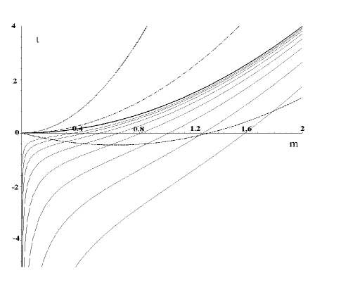
Figure 1: Complete gravitational collapse to a black hole for the case $t_{s}=m^{2}$. The thick solid curve is $t_{s}$, $t_{sc}=5m^{2}$ and is shown dotted. $t_{ah}=m^{2}-4m/3$ and is shown dashed. $\rho^{\prime}<0$ for $t<5m^{2}/3$ shown in the dash dot curve. The other curves are curves of constant $R$. This shows complete gravitational collapse to a black hole for a case that has a variable bang time. Junction can (but need not) be made onto the Schwarzschild vacuum at any $m>0$.

VII Conclusion

By using the effective gravitational mass as a coordinate in the LT solutions, a local sufficient condition for the development of a black hole has been given. This condition allows and invariantly defined non-vanishing range in central density cusps, the central feature of the LT solutions when used to match cosmological observations without invoking the cosmological constant. If one demands no density cusps in the initial conditions, then we have shown that the LT models never produce even locally naked singularities.