Soft evolution of multi-jet final states

Abstract:

We present a new framework for computing resummed and matched distributions in processes with many hard QCD jets. The intricate color structure of soft gluon emission at large angles renders resummed calculations highly non-trivial in this case. We automate all ingredients necessary for the color evolution of the soft function at next-to-leading-logarithmic accuracy, namely the selection of the color bases and the projections of color operators and Born amplitudes onto those bases. Explicit results for all QCD processes with up to $2\to 5$ partons are given. We also devise a new tree-level matching scheme for resummed calculations which exploits a quasi-local subtraction based on the Catani–Seymour dipole formalism. We implement both resummation and matching in the Sherpa event generator. As a proof of concept, we compute the resummed and matched transverse-thrust distribution for hadronic collisions.

1 Introduction

Jets play a central role in the physics program of the CERN Large Hadron Collider (LHC). The typical minimum value for jet transverse momenta considered in LHC analyses is of the order of 20 GeV, which is more than two orders of magnitude smaller than the center-of-mass energy, resulting in a huge phase space for jet production. Events with a high jet multiplicity are therefore copiously produced at the LHC [1, *Aad:2013ysa, *Khachatryan:2014zya].

Moreover, typical signatures of new-physics models include cascade decays of new heavy states producing relatively hard quarks and gluons, which seed hard jets. Accurate theoretical estimates of the related QCD multi-jet backgrounds are therefore essential. This has triggered intense activity in the QCD community, resulting in more and more accurate calculations of cross sections and differential distributions for multi-jet final states.

Leading order (LO) perturbative QCD calculations for multi-jet processes can automatically be performed for large multiplicities [4, *Cafarella:2007pc, 6]. Next-to-leading order (NLO) corrections have also reached a high level of automation [7, *Ossola:2006us, *Ellis:2007br, *Binoth:2008uq, *Berger:2008sj, *Bevilacqua:2011xh, *Cullen:2011ac, *Cascioli:2011va, *Hirschi:2011pa, *Badger:2012pg, *Actis:2012qn], and fully differential multi-jet cross sections are now available for pure QCD processes and electroweak ($W^{\pm}$, $Z$ and Higgs) boson production in association with up to five jets [18, *Bern:2013gka, *Badger:2013yda, *Cullen:2013saa].

Monte Carlo parton showers [22, *Sjostrand:1985xi, *Marchesini:1987cf], which describe the all-order evolution of QCD partons fully exclusively, have been extended beyond the strict collinear limit [25, *Giele:2007di, *Schumann:2007mg, *Platzer:2009jq] and even beyond the $1/N_{C}$ approximation [29, *Nagy:2012bt]. They can be merged with LO predictions for multi-jet events [31, *Mangano:2001xp, *Lonnblad:2001iq, *Krauss:2002up] and matched to NLO calculations [35, 36, *Frixione:2007vw] for over a decade. More recently, methods for combining next-to-leading order matched predictions of varying jet multiplicity have been devised [38, *Frederix:2012ps, *Lonnblad:2012ix], as well as matching methods at next-to-next-to leading order (NNLO) accuracy [41, *Hamilton:2013fea, *Hoeche:2014aia]. Dedicated Monte Carlo programs aimed at better describing jet production in the high-energy limit have also been developed [44].

Thus, the past years have brought substantial theoretical progress in multi-jet physics, both from the viewpoint of fixed-order calculations and parton showers, as well as the matching and merging of the two approaches. Another important aspect of QCD phenomenology is the all-order resummation of particular classes of observables or processes, beyond the leading-logarithmic (LL) accuracy, which is typical for parton showers. Event shapes in electron-positron, electron-proton and hadron-hadron collisions have been studied for a long time (see for instance [45, 46] and references therein) and a general framework for resumming event shapes at next-to-leading logarithmic (NLL) accuracy was developed in Refs. [47, *Banfi:2003je, *Banfi:2004nk, *Banfi:2004yd]. Very high logarithmic accuracy (N³LL) was achieved using Soft Collinear Effective Theory (SCET) for particular event shapes in $e^{+}e^{-}$ collisions [51, 52]. Inter-jet radiation and in particular its response to the presence of a jet veto has also received a lot of attention both from the theoretical [53, *Appleby:2003sj, 55, *Forshaw:2008cq, *Forshaw:2009fz, *DuranDelgado:2011tp, 59] and experimental [60, *ATLAS:2012al, *Aad:2014pua, *Chatrchyan:2012gwa] communities, primarily in the context of Higgs-boson studies [64, *Banfi:2012jm, *Banfi:2013eda, *Becher:2012qa, *Becher:2013xia, *Stewart:2013faa, *Boughezal:2013oha]. All-order analytical calculations have been performed recently for an increasing number of jet-substructure observables, including jet masses [71, *Dasgupta:2012hg, *Chien:2012ur, *Jouttenus:2013hs], other jet shapes [75, *Larkoski:2013paa, *Larkoski:2014uqa, *Larkoski:2014tva, *Larkoski:2014gra], sub-jet multiplicity [80] and grooming algorithms [81, *Dasgupta:2013via, *Larkoski:2014wba]. Recently, there has also been substantial progress towards achieving NNLL accuracy in threshold resummation for dijet production [84, *Hinderer:2014qta].

However, to our knowledge, all phenomenological studies that used all-order resummed results have been restricted to cases with four or less hard colored partons, i.e. $2\to 2$ QCD scattering in hadron-hadron collisions [86, *Dokshitzer:2005ig, 88, 89] . The reason for this deficiency in comparison to the enormous progress in fixed-order calculations is purely technical. While logarithmic terms associated to collinear emissions have a simple color structure, i.e. the Casimir operator of the jet under consideration, the color structure of soft-gluon emissions at large angles is more complex and, in particular, has a non-trivial matrix structure for $n\geq 4$ partons. Nevertheless, resummed calculations can in principle be written for an arbitrary number of hard colored legs, using, for instance, the formalism of Refs. [86, *Dokshitzer:2005ig, 90, 91, *Catani:1996vz, 93]. In order to perform an actual calculation, one then needs to define a suitable color basis for each partonic subprocess, and consequently find the matrix representation of all color insertions. The dimensionality of color bases rapidly increases with the number of legs. Algorithms to define them have been discussed in the literature, e.g. [94, 95, 96, 97]. However, when making use of a non-orthogonal basis, the efficient inversion of the matrix representing the color metric can pose a severe problem. In addition, the underlying Born matrix elements for the hard process must be decomposed in the chosen basis. One would clearly like to automate all these steps.

The main purpose of this study is to overcome these technical difficulties and provide a tool to perform soft-gluon resummation at NLL accuracy for processes with, in principle, arbitrarily many hard legs. In practice we have considered all contributions for up to $2\to 5$ processes. As detailed in Sec. 2, we achieve this by writing the resummed exponent in a suitable color basis and by decomposing the Born amplitudes using modified color-dressed recursive relations [98], as implemented in the Comix matrix-element generator [6], that is part of the Sherpa framework [99, *Gleisberg:2008ta].

In this paper, we also address the issue of matching the resummation to fixed-order calculations. In Sec. 3 we develop an automated LO matching scheme which makes use of modified dipole subtraction [91, *Catani:1996vz]. It circumvents the explicit expansion of the resummation formulae to a large extent and provides a quasi-local cancellation of the logarithmic contributions. We use the resummation of the transverse thrust in hadronic collisions as a first example to study the performance of our method. We finally summarize our work and indicate future directions in Sec. 4.

2 The soft function and its anomalous dimension

The main aim of this work is to define and implement NLL resummation for processes with an arbitrary number of hard partons. Despite the computational difficulties arising from the non-trivial color structure in soft-gluon radiation, one can formally write all-order resummed expressions in terms of abstract color operators [86, *Dokshitzer:2005ig, 90, 91, *Catani:1996vz, 93], which are then valid for an arbitrary number of hard legs.

The quantity we are interested in is the NLL “soft function” [86, *Dokshitzer:2005ig, 88]

$$\mathcal{S}(\xi)=\frac{\langle m_{0}|e^{-\frac{\xi}{2}\mathbf{\Gamma}^{\dagger}}e^{-\frac{\xi}{2}\mathbf{\Gamma}}|m_{0}\rangle}{\langle m_{0}|m_{0}\rangle}.$$ (1)

In the above equation, $|m_{0}\rangle$ denotes a vector in color space representing the Born amplitude, such that the color-summed squared matrix element is $|{\cal{M}}_{0}|^{2}=\langle m_{0}|m_{0}\rangle$. Therefore, Eq. (1) describes the soft gluon evolution of the Born amplitude from the hard scale of the process down to the low scale, set by the observable under consideration, thus resumming to all orders the logarithmic contributions encoded in the evolution variable $\xi$. Note that the soft function defined here and used throughout this paper does not contain any collinear logarithms and the evolution variable $\xi$, the precise functional form of which may depend on the observable at hand, is single-logarithmic. This is in contrast to alternative definitions also common in the literature. Moreover, to NLL considered here, the soft function depends on the strong coupling only through the variable $\xi$.

The soft function in Eq. (1) is defined in terms of the central object in our study: the soft anomalous dimension $\mathbf{\Gamma}$. Although much of the computational technology developed here can be applied to a variety of observables, in order to keep the presentation simple, we focus our discussion on global event shapes . For this class of observable, $\mathbf{\Gamma}$ can be written as

$$\mathbf{\Gamma}=-2\sum_{i<j}{\bf T}_{i}\cdot{\bf T}_{j}\,\ln\frac{Q_{ij}}{Q_{12}}+i\pi\sum_{i,j=II,FF}{\bf T}_{i}\cdot{\bf T}_{j}\,.$$ (2)

The first sum runs over all possible colored dipoles, with $Q_{ij}$ the respective invariant mass, i.e.

$$Q_{ij}^{2}=2\,p_{i}\cdot p_{j}.$$ (3)

The second sum in Eq. (2) is over the Coulomb (or Glauber) contributions between final–final (FF) and initial–initial (II) parton pairs. Note that the non-commutativity of $\mathbf{\Gamma}$ and $\mathbf{\Gamma}^{\dagger}$ prevents us from recombining the exponentials in Eq. (1) and leads to a physical effects from the Coulomb phase.

In order to make contact with the existing literature, we can evaluate Eq. (2) for the special case of $2\to 2$ scattering of massless partons. In this case, $Q_{12}=Q_{34}=\sqrt{s}$, $Q_{13}=Q_{24}=\sqrt{-t}$ and $Q_{14}=Q_{23}=\sqrt{-u}$, and the soft anomalous dimension becomes (see e.g. [47, *Banfi:2003je, *Banfi:2004nk, *Banfi:2004yd])

$$\mathbf{\Gamma} =-\left({\bf T}_{1}\cdot{\bf T}_{3}+{\bf T}_{2}\cdot{\bf T}_{4}\right)T-\left({\bf T}_{1}\cdot{\bf T}_{4}+{\bf T}_{2}\cdot{\bf T}_{3}\right)U,$$ (4)

where we have employed color conservation, i.e.

$$\left(\sum\limits_{i=1}^{4}{\bf T}_{i}\right)|m_{0}\rangle=0\,,$$ (5)

introduced the compact notation

$$T=\ln\frac{-t}{s}+i\pi\quad\text{and}\quad U=\ln\frac{-u}{s}+i\pi,$$ (6)

and dropped all contributions from abelian phases because they do not contribute to any cross sections.

Aiming for an automated evaluation of Eq. (1) for arbitrary processes, there are essentially three problems which need to be addressed:

• the color-basis definition and computation of the metric,

• the computation of the color operators ${\bf T}_{i}\cdot{\bf T}_{j}$, in the considered basis,

• the decomposition of the amplitude $|m_{0}\rangle$ in the considered basis.

The construction and implementation of an algorithm addressing all three items represents the core of this paper. This problem is closely related to the color decomposition of QCD amplitudes [101], which is typically written in the form

$$\mathcal{M}_{0}(1,{\alpha_{1}};\ldots;n,{\alpha_{n}})=\sum_{i}C^{(i)}(\alpha_{1},\ldots,\alpha_{n})\,m_{0}^{(i)}(1,\ldots,n)\;.$$ (7)

Here, $\mathcal{M}_{0}$ is the full amplitude for a set of external particles $1\ldots n$ with color assignments $\alpha_{1}\ldots\alpha_{n}$. The $C^{(i)}$ are color coefficients, and the $m_{0}^{(i)}$ are color-ordered partial amplitudes. The index $i$ labels the color orderings contributing to the color assignment. While the number of orderings and the related color coefficients change with the color basis [102, *DelDuca:1999rs, 104], the partial amplitudes are unique, gauge-invariant objects depending only on the particle momenta. They are given by sums of planar diagrams computed in the large-$N_{C}$ limit [105]. One may consider Eq. (7) the projection of the Born amplitude onto a given color-basis element, $\mathcal{M}_{0}(\alpha)=\langle c_{\alpha}|m_{0}\rangle$. This will be discussed in more detail in the following.

2.1 Non-orthogonal color bases

We first define our notation for color bases. As we are going to work with bases which are not necessarily orthogonal (for a discussion about this topic see also Refs. [106, 107, 108]), we start by defining basis vectors $|c_{\alpha}\rangle$ and introduce the (non-diagonal) color metric, and its inverse

$$\langle c_{\alpha}|c_{\beta}\rangle=c_{\alpha\beta}\neq\delta_{\alpha\beta}\quad\quad c^{\alpha\beta}=(c_{\alpha\beta})^{-1}\,.$$ (8)

Note that $c_{\alpha\gamma}c^{\gamma\beta}=\delta_{\alpha}^{\;\;\beta}$ by construction. The basis vectors $|c_{\alpha}\rangle$ span a complete (possibly over-complete) set of elements which we leave undetermined for the moment. We will adopt the convention of referring to $c^{\alpha\beta}$ as the inverse metric.

Let us consider a general tensor $H^{\beta\gamma}$ expressed in the non-orthogonal $c$-basis. Color invariants are computed by contracting with the metric, and we define in particular the color trace as ${\rm Tr}(cH)=c_{\alpha\beta}H^{\alpha\beta}$. Indices between the $c$-basis and its dual are raised and lowered with the metric. Tensors transforming with mixed indices are interpreted as $H^{\;\;\beta}_{\alpha}\equiv H_{\alpha\gamma}c^{\gamma\beta}$.

The soft function from Eq. (1) written in matrix notation reads

$$\mathcal{S}(\xi)\;\;=\;\;\frac{{\rm Tr}\left(H{\rm e}^{-\frac{\xi}{2}\Gamma^{\dagger}}c\,{\rm e}^{-\frac{\xi}{2}\Gamma}\right)}{{\rm Tr}\left(cH\right)}\;\;=\;\;\frac{c_{\alpha\beta}H^{\gamma\sigma}\mathcal{G}^{\dagger}_{\gamma\rho}c^{\rho\beta}c^{\alpha\delta}\mathcal{G}_{\delta\sigma}}{c_{\alpha\beta}H^{\alpha\beta}},$$ (9)

where $c_{\alpha\beta}H^{\alpha\beta}=\langle m_{0}|m_{0}\rangle$ now represents the color-summed Born matrix element squared. The matrix $\mathcal{G}$ is the exponential of the soft anomalous dimension matrix, which due to the non-orthogonal nature of the $c$-basis, takes the form

$$\mathcal{G}_{\alpha\beta}(\xi)\;\;=\;\;c_{\alpha\gamma}\exp\left(-\frac{\xi}{2}\,\Gamma_{\;\;\beta}^{\gamma}\right)\;\;=\;\;c_{\alpha\gamma}\exp\left(-\frac{\xi}{2}\,c^{\gamma\delta}\,\Gamma_{\delta\beta}\right).$$ (10)

A significant amount of recent work has focused on improving the basis construction, with certain advantages and disadvantages for each approach. In [95], a complete trace basis was discussed which followed from combining the connected fundamental representation color tensors appearing in the tree-level hard matrix element with the disconnected color structure required by soft-gluon exchange. The construction of this basis for an arbitrary process was automated in [96]. In [97] a general orthonormal basis was constructed, which was shown to be minimal in elements for a given process.

In this work we follow a different approach. Instead of constructing new optimized color bases, we rely on existing ones and circumvent the problem of over-completeness in an automated fashion by extending the dimensionality of color space. This method, and the alternative approach of dimensional reduction, will be discussed in more detail in Sec. 2.2. In order to select the color bases to start with, we use the following guiding principles:

1. Minimal partial-amplitude count: The components $\mathcal{M}(\alpha)=\langle c_{\alpha}|m_{0}\rangle$ should depend on as few partial amplitudes as possible.

2. Physical color states: The basis vectors should represent physical color states. This disqualifies bases containing singlet gluons, for example.

3. Minimality of the basis: Although we will also use over-complete bases, we require the dimension of the basis to be as low as possible.

The trace basis [101] for processes with quarks and the adjoint basis [102, *DelDuca:1999rs] for processes with only gluons satisfy our guiding principles, and we choose to implement them. However, subtleties arise because these bases can be over-complete. In this respect, we note that exponentiation via Eq. (10) requires the computation of the inverse color metric $c^{\alpha\beta}$. Thus, $c^{\alpha\beta}$ must be non-singular for general $N_{C}$. At $N_{C}=3$ it may be singular if the corresponding metric $c_{\alpha\beta}$ contains representations with weight proportional to $N_{C}-3$. In this case the inversion may be computed with $N_{C}=3+\epsilon$ colors. More on this issue appears in Sec. 2.2.

Processes including quarks

The complete basis for processes including quarks follows from color connecting all same flavor quark lines while attaching gluons in the form of fundamental-representation matrices. For example, in the case of a single quark pair the decomposition at tree-level is [101]

$$\mathcal{M}_{0}(1,{i_{1}};2,{a_{2}};\ldots;n,{j_{n}})=\sum_{\sigma\in P(n-2)}(T^{a_{\sigma_{2}}}\ldots T^{a_{\sigma_{n-1}}})_{i_{1}}^{j_{n}}\,m_{0}(1,\sigma_{2},\ldots,\sigma_{n-1},n)\;.$$ (11)

The sum runs over all $(n-2)!$ permutations of the particle labels $2\ldots n-1$, which represent the gluons. Decompositions for processes with multiple quark lines are qualitatively similar and can be found in the literature. In the general case, the decomposition includes disconnected quark lines, arising from soft gluon exchange, and disconnected gluon lines, which appear for processes with 2 or more gluons. Similar terms appear at higher loops in fixed-order calculations.

An important simplification is that any basis with the same number of $q\bar{q}$ pairs (taking flavor labels as all incoming) and gluons is the same, modulo crossings. This suggests that for a given set of particle flavors, the resummation may be carried out for a fixed flavor ordering. In practice we implement this by always computing ${\bf\Gamma}$ in the same flavor arrangement $\{q,\bar{q},g\}$ so that the first sum in Eq. (2) is always in order.

We keep track of the map to the physical process by labeling incoming and outgoing for the purpose of assigning the Coulomb phase. This means that the matrices ${\bf T}_{i}\,\cdot\,{\bf T}_{j}$ only need to be computed once for all processes involving the same number of quarks and gluons.

Purely gluonic processes

There are multiple options of dealing with purely gluonic processes. The first and oldest of them is the trace basis, described in Ref. [101]. The color decomposition of tree-level amplitudes reads

$$\mathcal{M}_{0}(1,{a_{1}};\ldots;n,{a_{n}})=\sum_{\sigma\in P(n-1)}{\rm Tr}(T^{a_{1}}T^{a_{\sigma_{2}}}\ldots T^{a_{\sigma_{n}}})\,m_{0}(1,\sigma_{2},\ldots,\sigma_{n})\;.$$ (12)

The sum runs over all $(n-1)!$ permutations of the particle labels $2\ldots n$. In the context of resummation, we must add the non-vanishing color disconnected components containing multiple gluon traces, which also appear at higher loops in fixed-order calculations.

A subtlety arises due to the reflection symmetry of the partial amplitudes, $m_{0}(1,2,3,\ldots,n)=m_{0}(1,n,\ldots,3,2)$, which holds for the corresponding soft gluon evolved amplitudes as well. The basis elements corresponding to permutation $123\ldots n$ and $n\ldots 321$ can be combined due to this symmetry, so that the number of connected basis elements for general $N_{C}$ is reduced by a factor two.

The adjoint ($f$-) basis [102, *DelDuca:1999rs] corresponds to the remaining basis vectors after applying the Kleiss-Kuijf relations [109]. Equation (12) reduces to

$$\mathcal{M}_{0}(1,{a_{1}};\ldots;n,{a_{n}})=\sum_{\sigma\in P(n-2)}(F^{a_{\sigma_{2}}}\ldots F^{a_{\sigma_{n-1}}})_{a_{1}a_{n}}\,m_{0}(1,\sigma_{2},\ldots,\sigma_{n-1},n)\;,$$ (13)

where the sum runs over only $(n-2)!$ permutations, corresponding to the new basis elements. As with the trace basis, we add the disconnected components, which starting at 6 gluons may also feature $4$ gluons connected via adjoint tensors.

2.2 Elimination of $N_{C}=3$ pathologies

Although advantageous from many points of view, both the trace and adjoint bases for high-multiplicity processes turn out to be over-complete. As a consequence, the matrices representing the corresponding color metric, defined as in Eq. (8), have null eigenvalues at $N_{C}=3$. However, the fact that the inverse metric at $N_{C}=3$ is often singular is an artefact of calculating $c^{\alpha\beta}$ and $\mathbf{\Gamma}$ separately, since maintaining the full $N_{C}$ dependence the resulting $\mathcal{S}$-function is always finite. Keeping the $N_{C}$ dependence explicit becomes computationally impractical for large multiplicity. Here we outline two strategies to overcome these limitations.

Dimensional Reduction

The simplest solution is to reduce the size of the color basis, in particular, if we bear in mind the freedom to reparameterize the basis elements with no tree-level Born contribution. These components only enter $\mathcal{S}$ through contractions with the inverse metric and can therefore be reshuffled for convenience.

More precisely, for a basis with $m$ Born proportional and $n-m$ non-Born elements $\{c_{0},\cdots,\,c_{m-1},\,c_{m},\,c_{m+1},\cdots,\,c_{n-1},\,c_{n}\}$, we examine the situation where there is a single zero eigenvalue at $N_{C}=3$ in the color metric. In other words, the basis decomposes into $n-1$ non-vanishing irreducible representations. A simple procedure for reducing the color space then corresponds to the new basis $\{c_{0},\cdots,\,c_{m-1},\,c_{m}+c_{n},\,c_{m+1}+c_{n},\cdots,\,c_{n-1}+c_{n}\}$, where we normalise new elements accordingly.

While for simpler processes this procedure is straight-forward (see section A.2), for the general case it is hard to automate, and therefore we choose a different approach.

Numerical Inversion with $N_{C}=3+\epsilon$

We adopt a solution which avoids adjusting the dimensionality of the basis, and therefore requires no a priori group theory knowledge on the color decomposition of a given process. This is the simplest solution practically, though there is clearly an efficiency loss due to carrying through non-contributing color directions.

We state the necessary claims here while proofs may be found in App. A.1. First, we note that the metric is always invertible for $N_{C}=3+\epsilon$ with $\epsilon>0$. We can separate the singular from the regular part of the inverse color metric as

$$c^{\alpha\beta}_{3+\epsilon}=c^{\alpha\beta}_{R}+\frac{1}{\epsilon}\tilde{c}^{\,\alpha\beta}\,.$$ (14)

The singular part of the inverse metric is in the null-space of all color products evaluated at $N_{C}=3$

$$\tilde{c}^{\,\alpha\beta}({\bf T}_{i}\cdot{\bf T}_{j})_{\beta\gamma}={\bf{0}}^{\alpha}_{\;\;\gamma}\,,$$ (15)

which guarantees that

$$\mathcal{S}(\xi)_{N_{C}=3+\epsilon}=\mathcal{S}(\xi)_{N_{C}=3}+{\mathcal{O}}{(\epsilon)}.$$ (16)

We find that the error introduced in the resummation is ${\mathcal{O}}(\epsilon)$ which may be taken sufficiently (arbitrarily) small in practice (theory).

2.3 Computation of the hard matrix

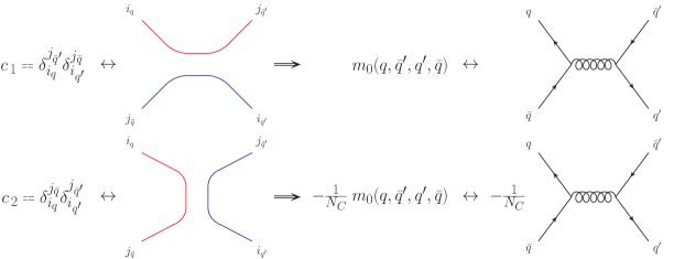
Figure 1: Sketch of color basis vectors and their corresponding projections of Born matrix elements for $q\bar{q}\to q^{\prime}\bar{q}^{\prime}$ scattering. All flavors in the figure are taken as outgoing.

A key ingredient for the computation of the soft function Eq. (9) is the hard matrix, which is formed by projections of the Born amplitudes onto color basis vectors, $H^{\alpha\beta}=\langle m_{0}|c_{\alpha}\rangle\langle c_{\beta}|m_{0}\rangle$. Consider, for instance, the trivial case of $q\bar{q}\to q^{\prime}\bar{q}^{\prime}$ scattering, where $q$ and $q^{\prime}$ represent two different quark flavors. The Born matrix element factorizes into a purely kinematical part, which stems from the $s$-channel diagram squared, and color coefficients defining the actual matrix structure. This is shown in Fig. 1. However, in any non-trivial case, multiple diagrams appear, which contribute differently to the different matrix elements, such that the hard matrix has a non-trivial dependence on the Born kinematics. In particular, same-flavor quark processes like $q\bar{q}\to q\bar{q}$ scattering have partial amplitudes where both $s$- and the $t$-channel diagrams contribute because of the $1/N_{C}$ suppressed term in the Fierz identity. This is sketched in Fig. 2. Automating the computation of $H^{\alpha\beta}$ requires an algorithm that allows us to easily access these partial amplitudes.

We solve this problem with the help of Comix [6], a matrix-element generator that computes multi-parton amplitudes using color-dressed recursive relations [98]. Comix is part of the Sherpa framework [99, *Gleisberg:2008ta]. As Comix allows us to define a color configuration in the large-$N_{C}$ limit, it is trivial to obtain color-ordered partial amplitudes. However, these are not necessarily sufficient to compute the entries of the hard matrix directly.

Take for example $q\bar{q}\to q\bar{q}$ scattering, as depicted in Fig. 2. The two amplitudes needed for the hard matrix are shown schematically on the first and the second line. To compute them individually, we can use a colorful matrix element that is projected onto the correct set of diagrams by selecting external colors appropriately. Using the color-dressed Feynman rules from [98], the amplitudes on the right-hand side, including their prefactors, are generated by choosing the colors on the left-hand side. If the number of colors is fixed to three, this leads to problems for amplitudes with more than three fundamental color indices, as non-planar diagrams start to appear. These are removed by working at $N_{C}\to\infty$. Taking this limit, however, would eliminate the second diagram on the first line and the first diagram on the second line, because the gluon propagator does not have a $1/N_{C}$ contribution. The problem is solved by keeping this term when taking the limit. This modification is implemented at the vertex level by changing the color-dressed Feynman rules such that $U(1)$ gluons couple to quark lines also in the large-$N_{C}$ limit, while evaluating the corresponding $1/N_{C}$ term in the Fierz identity with $N_{C}=3$.

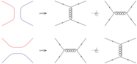
Figure 2: Sketch of color basis vectors and their corresponding projections of Born matrix elements for $q\bar{q}\to q\bar{q}$ scattering. In comparison to Fig. 1, there is both an s- and a t-channel diagram, both of which contribute to each projection with different weight.

We note that it is possible to add the relevant one-loop partial amplitudes and extend this algorithm beyond the tree level. This will provide the hard matrix one order higher, which is needed in order to achieve higher logarithmic accuracy in the resummation.

2.4 Validation against multi-parton matrix elements

In order to check the construction of the color metric for the employed bases and the correctness of the corresponding decomposition of the hard matrix for multi-parton amplitudes, we compare our results against exact real-emission matrix elements considering soft but non-collinear kinematics for the emitted gluon. Starting from an $n$-parton state with momenta $p_{1},\ldots,p_{n}$ we assume the emitted gluon to carry additional momentum $p_{s}$, with $|p_{s}|=k_{s}$. We choose a particular kinematic configuration, where the final-state momenta resemble a circle in the transverse plane, i.e.,

$$p_{1}=E(1,0,0,1)\,,$$

$$p_{2}=E(1,0,0,-1)\,,$$

$$p_{3}=E_{n}(1,\cos(\phi_{n3}+\phi_{H}),\sin(\phi_{n3}+\phi_{H}),0)\,,$$

$$p_{4}=E_{n}(1,\cos(\phi_{n4}+\phi_{H}),\sin(\phi_{n4}+\phi_{H}),0)\,,$$

$$\vdots$$

$$p_{n}=E_{n}(1,\cos(\phi_{nn}+\phi_{H}),\sin(\phi_{nn}+\phi_{H}),0)\,,$$

$$p_{s}=k_{s}(1,\cos\phi_{s},\sin\phi_{s},0)\,,$$ (17)

with $E_{n}=2E/(n-2)$ and $\phi_{nm}=\pi(2m-3)/(n-2)$. The momenta $p_{1}$ to $p_{n}$ can then be used directly to evaluate the $n$-parton amplitude. For the computation of the $(n+1)$-parton process we assume the recoil of the emitted soft-gluon to be absorbed by the dipole spanned by partons $3$ and $4$. The momenta of partons $3$ and $4$ that enter the $(n+1)$-parton amplitude are then given by

$$p^{\prime}_{3}=p_{3}-p_{s}+\frac{p_{3}\cdot p_{s}}{p_{4}\cdot(p_{3}-p_{s})}p_{4}\,,$$

$$p^{\prime}_{4}=\left(1-\frac{p_{3}\cdot p_{s}}{p_{4}\cdot(p_{3}-p_{s})}\right)p_{4}\,.$$ (18)

We define with $R_{s}$ the inverse ratio between an $n+1$-parton matrix element squared and its “sum-over-dipoles” approximation

$$R_{s}= \frac{\alpha_{\rm S}}{\pi}\text{Tr}\left[H_{n}\sum_{i<j}{\bf T}_{i}\cdot{\bf T}_{j}\frac{p_{i}\cdot p_{j}}{p_{i}\cdot p_{s}\,p_{j}\cdot p_{s}}\right]\frac{1}{\text{Tr}\;\left(c\,H_{n+1}\right)}.$$ (19)

The QCD coupling $\alpha_{\rm S}$ is assumed fixed here. Factorization of QCD matrix elements implies that in the limit of soft-gluon kinematics, i.e., $\lambda_{s}=k_{s}/(2E)\to 0$, we have

$$\lim_{\lambda_{s}\to 0}R_{s}=1.$$ (20)

This result is in fact independent of the underlying Born kinematics, and in particular independent of the angle $\phi_{H}$ through which we rotate our hard-parton configuration, Eq. (2.4). Depending on $\phi_{H}$, the value of $R_{s}$ for finite $\lambda_{s}$ may be larger or smaller than one. Taking the limit in (20), we provide a strong consistency check on the elements of $\mathbf{\Gamma}$ and $H_{n}$ for the $n$-parton process as well as $c$ and $H_{n+1}$ for the $n+1$ parton configuration. This applies to elements which have a non-vanishing hard contribution.

In order to expose this property of the full matrix element, we sample over $\phi_{H}$ in discrete steps assuring that the momentum $p_{s}$ does not get collinear to any other parton. This is sufficiently satisfied by requiring that $\phi_{H}$ is not an integer multiple of $\phi_{s}$. In practice we take $\phi_{s}=\pi/7$, and sample $\phi_{H}=N\pi/10$ over $N=0,\dots,9$.

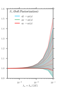
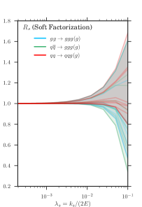
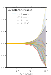
Figure 3: (Left) Ratio of the sum-over-dipole dressed $4$-parton approximation to the exact $5$-parton matrix elements for different partonic subprocesses, cf. Eq. (20). (Middle) $R_{s}$ ratio for sum-over-dipole dressed $5$-parton over full $6$-parton configurations. (Right) Same but for $6/7$-parton matrix elements.

In Fig. 3 we display the results of our checks for soft-gluon emission off $4$- (left), $5$-parton (middle) and $6$-parton (right) amplitudes. The last case provides a non-trivial check also on the $7$-parton color metric and hard matrix, entering through the denominator of Eq. (20). For completeness we collect in App. A.3 the properties of the color bases used for the various processes. By rotating the respective Born kinematics on the circle in the transverse plane, we can verify that the individual coefficients of each dipole are exactly matched in the full matrix element as $\lambda_{s}\to 0$. For a specific phase-space point these coefficients could be individually very small thus not providing a sufficient test. The results show a strong dependence on the underlying kinematic configuration in addition to the considered parton flavors. However, for sufficiently small $\lambda_{s}$ in all cases $R_{s}$ approaches unity, proving correctness of the ingredients for the soft function $\mathcal{S}$.

2.5 Soft evolution of multi-parton squared amplitudes

Having proven correctness of our color-metric evaluation and the corresponding hard-matrix decomposition, we shall now study the full soft function ${\mathcal{S}}(\xi)$ given in Eq. (9) for multi-parton processes. In particular we probe the dependence on the evolution variable $\xi$ and compare to the limiting case of $N_{C}\to\infty$, that closely resembles the approximation used in parton-shower simulations. While the $N_{C}=\infty$ anomalous dimension is computed explicitly in the trace basis, it amounts to only a non-vanishing contribution to ${\bf T}_{i}\cdot{\bf T}_{j}$ for basis elements which have partons $i$ and $j$ color adjacent.

We begin by computing $\mathcal{S}(\xi)$ for several multiplicities at benchmark kinematics, that lie on a circle in the transverse plane at $z=0$. For the $2\to n$ processes we parameterize the momenta as

$$p_{1} =E(1,0,0,1)\,,$$

$$p_{2} =E(1,0,0,-1)\,,$$

$$p_{3} =E_{n}(1,\cos\phi_{n3},\sin\phi_{n3},0)\,,$$

$$p_{4} =E_{n}(1,\cos\phi_{n4},\sin\phi_{n4},0)\,,$$

$$\vdots$$

$$p_{n} =E_{n}(1,\cos\phi_{nn},\sin\phi_{nn},0)\,,$$ (21)

where again $E_{n}=2E/(n-2)$ and $\phi_{nm}=\pi(2m-3)/(n-2)$. The soft function $\mathcal{S}$ depends on the kinematics merely through ratios of momentum invariants (cusp angles), such that when considering fixed $\alpha_{\rm S}$ the direct dependence on $E_{n}$ vanishes.

    

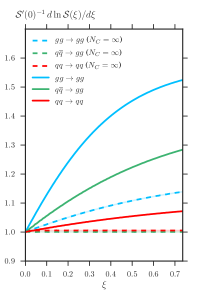
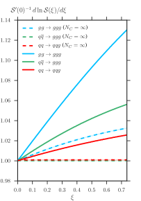
Figure 4: Dependence of the soft function $\mathcal{S}$ on the evolution variable $\xi$ for $2\to 2$ (left) and $2\to 3$ (right) parton configurations. For all processes parton momenta on a circle in the transverse plane at $z=0$ are considered.

    

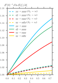
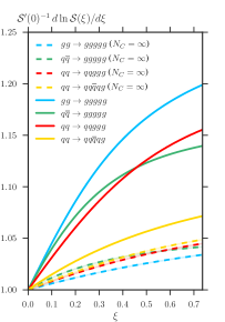
Figure 5: Dependence of the soft function $\mathcal{S}$ on the evolution variable $\xi$ for $2\to 4$ (left) and $2\to 5$ (right) parton configurations. For all processes parton momenta on a circle in the transverse plane at $z=0$ are considered.

In Fig. 4 and Fig. 5 we present results for the $\xi$-dependence of the soft function for various parton channels, both for $N_{C}=3$ (solid curves) and for the limit $N_{C}\to\infty$ (dashed curves). Depicted is the variation of $\ln{\mathcal{S}}(\xi)$ with $\xi$, where we scaled each curve such that it intersects with the ordinate at one. We observe a non-trivial $\xi$ dependence for all processes when considering the full-color treatment. For the given phase-space configurations the full result shows a stronger variation with $\xi$ than the large-$N_{C}$ estimate. This originates from taking into account all off-diagonal elements in the soft anomalous dimension. In particular for processes involving gluons the limit $N_{C}\to\infty$ approximates the full result poorly.

Let us discuss the general behaviour of our results in the large-$N_{C}$ case. In this case, all non-diagonal entries of the soft anomalous dimension vanish and we can simply write

$$\frac{1}{\mathcal{S}^{\prime}(0)}\frac{d\log\mathcal{S}(\xi)}{d\xi}=\left(\dfrac{\sum_{i=1}^{n}h_{ii}}{\sum_{i=1}^{n}\lambda_{i}\,h_{ii}}\right)\dfrac{\sum_{i=1}^{n}h_{ii}\lambda_{i}\exp(\lambda_{i}\xi)}{\sum_{i=1}^{n}h_{ii}\exp(\lambda_{i}\xi)}\qquad(\text{at large\,-$N_{C}$})$$ (22)

for an $n$-dimensional color space where $\lambda_{i}$ and $h_{ii}$ are the diagonal entries of $\Gamma_{\alpha\beta}$ and $H^{\alpha\beta}$ respectively. Both $\lambda_{i}$ and $h_{ii}$ are positive because they correspond to non-interfering squared amplitudes. Consequently, Eq. (22) is a monotonically increasing function $\xi$, for all underlying Born configurations. However, at finite $N_{C}$, the full matrix structure persists and the behaviour is not neccesarily monotonic due to off-diagonal interfering contributions.

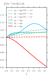
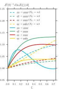
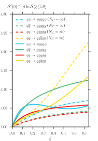
Figure 6: Soft function for $2\to 3$ (left), $2\to 4$ (middle) and $2\to 5$ (right) parton configurations, for kinematics with all final-state momenta in the plane of the beam.

To also check kinematic configurations with particles at non-zero rapidity, we considered the above kinematics but rotated by an angle $\pi/2$ about the $y$-axis. This results in momenta that span a circle in the $y-z$ plane at $x=0$. The corresponding results can be found in Fig. 6. Again, while the behaviour for $N_{C}\to\infty$ are necessarily monotonically increasing functions of $\xi$ this is not true for finite $N_{C}$, due to non-vanishing interference effects of different color flows. Accordingly, the large-$N_{C}$ approximation can in general also result in an overestimate of the soft function. To properly account for the highly non-trivial dependence on the parton kinematics and the evolution variable the soft function needs to be evaluated with its full color dependence, i.e. $N_{C}=3$. However, to fully quantify the importance of finite-$N_{C}$ effects not just the soft-function contribution but the full physical observable needs to be considered.

3 Towards phenomenology

In the first part of this paper, we have presented a new method to deal with the soft evolution of processes with many colored legs that provides a high degree of automation. Moreover, we have realized an implementation of this method that uses color-partial amplitudes extracted from the matrix-element generator Comix and evolves them according to the soft anomalous dimension Eq. (2), thus obtaining an efficient way of evaluating the soft function given in Eq. (1).

The aim of this second part is to create a framework in which the soft function $\mathcal{S}$ in Eq. (1) can be used for phenomenological studies. Let us generically call $v$ an observable that measures the “distance” from the lowest-order kinematics. In the context of jet studies, $v$ can be thought of as an observable describing internal jet properties, e.g. masses, angularities, energy correlation functions) or as an observable measuring the radiation outside the leading jets, e.g. event shapes or inter-jet radiation. When $v$ is small, logarithms $L=\ln\frac{1}{v}$ are large and resummation becomes a more efficient organization of the perturbative expansion than fixed-order perturbation theory. Furthermore, we have to consistently match the two approaches to obtain reliable predictions for the entire range of the observable $v$:

$$\frac{d\sigma^{\text{matched}}}{dv}=\frac{d\sigma^{\text{resummed}}}{dv}+\left(\frac{d\sigma^{\text{fixed-order}}}{dv}-\frac{d\sigma^{\text{expanded}}}{dv}\right).$$ (23)

The first term in the expression above is computed to some logarithmic accuracy, typically next-to-leading log (NLL) but not infrequently to NNLL, while the second one is computed at a given order in the strong coupling (state of the art is typically NLO). The last term represents the expansion of the resummed distribution to NLO and avoids double counting. The last two terms are affected by large logarithms and are in fact separately divergent in the limit $v\to 0$. However, their combination yields a finite remainder, called the matching term. Although conceptually trivial, computing the matching term is often numerically inefficient because it involves the separate evaluation of fixed-order contribution and expanded resummation in regions of phase space corresponding to soft and/or collinear emissions. It would be preferable to generate the finite remainder directly.

3.1 Resummed distributions

Resummed calculations are usually performed for the so-called cumulative distribution, i.e. the integral of the differential distribution up to a certain value $v$ of the observable under consideration:

$$\frac{d\Sigma(v)}{d\mathcal{B}} =\frac{1}{\sigma}\int_{0}^{v}\frac{d^{2}\sigma}{d\mathcal{B}dv^{\prime}}dv^{\prime}$$

$$=\sum_{\begin{subarray}{c}\text{partonic}\\ \text{configurations}\\ \delta\end{subarray}}\frac{d\sigma_{0}^{(\delta)}}{d\mathcal{B}}e^{Lg_{1}^{(\delta)}(\alpha_{s}L)+g_{2}^{(\delta,\mathcal{B})}(\alpha_{s}L)+\dots}\left[1+{\cal O}(\alpha_{\rm S})\right],$$ (24)

where $d\mathcal{B}$ indicates that the expression above is fully differential in the Born kinematics. Here we focus our attention on the NLL approximation of $\ln\Sigma$, i.e. we consider the functions $g_{1}^{(\delta)}$ and $g_{2}^{(\delta,\mathcal{B})}$ in Eq. (3.1), while dropping the non-logarithmic term in square brackets. The inclusion of this constant contribution is necessary in order to achieve what often is referred to as NLL^′ accuracy. We note that to this logarithmic accuracy such contribution, although flavor-sensitive, can be averaged over the different color flows. Furthermore, we note that this constant term can be extracted from NLO calculations as implemented, for instance, with the Powheg method [36, *Frixione:2007vw], which has been automated in the Sherpa framework in Ref. [110] . For our discussion, we follow the formalism developed in the context of the program Caesar  [47, *Banfi:2003je, *Banfi:2004nk, *Banfi:2004yd], which allows one to resum global event shapes in a semi-automated way. With a couple of generalizations, the Caesar framework is sufficient for our purposes. Furthermore, we will also briefly discuss some differences in the structure of the resummation that arise when dealing with non-global observables [111, *Dasgupta:2002bw] at the end of this section.

We consider processes which at Born level feature $n$ hard massless partons (legs) and $m$ color singlets (e.g. photons, Higgs or electroweak bosons) and we denote the set of Born momenta with $\{p\}$. Following Refs. [47, *Banfi:2003je, *Banfi:2004nk, *Banfi:2004yd] we consider positive-definite observables $V$ that measure the difference in the energy-momentum flow of an event with respect to the Born configuration, where $V(\{p\})=0$. For a single emission with momentum $k$, which is soft and collinear to leg $l$, the observable $V$ is parametrized as follows 

$$V\left(\{\tilde{p}\};k\right)=d_{l}\left(\frac{k_{t}^{(l)}}{Q}\right)^{a}e^{-b_{l}\eta^{(l)}}g_{l}\left(\phi^{(l)}\right),$$ (25)

where $k_{t}^{(l)}$, $\eta^{(l)}$ and $\phi^{(l)}$ denote transverse momentum, rapidity and azimuth of the emission, all measured with respect to parton $l$. $Q$ is the hard scale of the process which we set equal to the partonic centre of mass energy, i.e. $Q^{2}=s$. It is then possible to write the resummed exponent in Eq. (3.1) in terms of the coefficients $a$, $b_{l}$, $d_{l}$ and $g_{l}(\phi)$ that specify the behavior of the observable in the presence of a soft and collinear emission.

In particular, while the LL function $g_{1}^{(\delta)}$ is diagonal in color, one of the contributions that enter the NLL function $g_{2}^{(\delta,\mathcal{B})}$ is precisely the soft function, which, as discussed in Sec. 2, has a matrix structure in color space, with complexity that increases with the number of hard partons. Explicit formulae are collected in App. B. The results of Sec. 2 provide an automated way of computing these contributions, thus extending the applicability of the Caesar framework to processes with an (in principle) arbitrary large number of hard partonic legs.

We conclude this discussion with a few remarks on non-global observables [111, *Dasgupta:2002bw]. Non-global logarithms arise for those observables that have sharp geometrical boundaries in phase space. They originate in wide-angle soft gluons that lie outside the region where the observable is measured, re-emitting softer radiation back into that region. The Caesar framework presented above is not sufficient to deal with this case and new ingredients need to be introduced. Most noticeably, the NLL function $g_{2}^{(\delta,\mathcal{B})}$ receives a new contribution coming from correlated gluon emission . Because of their soft and large-angle nature, non-global logarithms have a complicated color structure. However, for phenomenological purposes, their resummation can be performed in the large-$N_{C}$ limit [111, *Dasgupta:2002bw, 114, 115], thus trivializing the color structure again. Recent studies suggest a way of performing this resummation at finite $N_{C}$ [116]. We believe that the methodology for performing all-order calculations with many hard legs can also prove useful in the application of those methods to LHC phenomenology. However, we leave this investigation for future work. Finally, we point out that while the color structure of the soft anomalous dimension $\mathbf{\Gamma}$ for non-global observables is formally the same as in Eq. (2), the coefficients of the ${\bf T}_{i}\cdot{\bf T}_{j}$ are observable-dependent, because of non-trivial limits for the azimuth and rapidity integrals.

3.2 Automated matching

In order to avoid double counting when matching a resummed calculation to a fixed-order one, we need to consider the expansion of the resummation. In this paper, we are concerned with matching to tree-level matrix elements, thus we have to consider the expansion of the NLL resummed distribution to $\mathcal{O}\left(\alpha_{\rm S}\right)$

$$\frac{d}{dL}\frac{d\Sigma^{(\delta)}}{d\mathcal{B}}=\frac{2\alpha_{\rm S}}{\pi}\frac{d}{dL}\left[\frac{G_{12}}{2}L^{2}+G_{11}L\right]+\mathcal{O}\left(\alpha_{\rm S}^{2}\right),$$ (26)

with $\alpha_{\rm S}=\alpha_{\rm S}(\mu_{R}^{2})$ and $L=\ln\left(1/v\right)$.

If the resummation is performed within the Caesar formalism, which is summarized for convenience in App. B, one is able to expressed the coefficients $G_{12}$ and $G_{11}$ in terms of the coefficients that parametrize the observable in Eq. (25). An explicit calculation leads to

$$G_{12}= -\sum_{l=1}^{n}\frac{C_{l}}{a(a+b_{l})}$$

$$G_{11}= -\left[\sum_{l=1}^{n}C_{l}\left(\frac{B_{l}}{a+b_{l}}+\frac{1}{a(a+b_{l})}\left(\ln\bar{d}_{l}-b_{l}\ln\frac{2E_{l}}{Q}\right)+\frac{1}{a}\ln\frac{Q_{12}}{Q}\right)\right.$$

$$+\left.\frac{1}{a}\frac{{\rm Re}[\Gamma_{\alpha\beta}]\,H^{\alpha\beta}}{c_{\alpha\beta}H^{\alpha\beta}}+\sum_{l=1}^{n_{\text{initial}}}\frac{\int_{x_{l}}^{1}\frac{dz}{z}P_{lk}^{(0)}\left(\frac{x_{l}}{z}\right)q^{(k)}(z,\mu_{F}^{2})}{2(a+b_{l})q^{(l)}(x_{l},\mu_{F}^{2})}\right]\,.$$ (27)

Our aim is to compute $G_{12}$ and the first term in $G_{11}$ by integrating collinear splitting functions in a Monte-Carlo approach over suitably defined regions of phase space. This procedure is similar to next-to-leading order subtraction techniques. It allows to combine the matching terms with real-emission matrix elements point-by-point in the real-emission phase space, and provides therefore a quasi-local cancellation of large logarithms in the matching. We use an existing implementation of the Catani–Seymour dipole-subtraction method in Sherpa  [117] as the basis for our implementation. The remaining terms proportional to $C_{l}$ in $G_{11}$ are generated by using the color-correlated Born amplitudes only and multiplying with the analytic expression for $\log\bar{d}_{l}-b_{l}\ln(2E_{l}/Q)$ (or $\log(Q_{12}/Q)$) and the relevant prefactors. The generation of the second line in Eq. (3.2) is described in detail below.

The dipole-subtraction method of Ref. [91, *Catani:1996vz] is based on the soft and collinear factorization properties of tree-level matrix elements. In the collinear limit we can write

$$\begin{split}&|\mathcal{M}_{0}(1,\ldots,i,\ldots,j,\ldots,n)|^{2}\;\overset{i,j\to\text{collinear}}{\longrightarrow}\\ &\quad\frac{8\pi\mu^{2\varepsilon}\alpha_{s}}{2p_{i}p_{j}}\,\langle m_{0}(1,\ldots,ij,\ldots,n)|\,\hat{P}_{ij,i}(z,k_{T},\varepsilon)\,|m_{0}(1,\ldots,ij,\ldots,n)\rangle\;.\end{split}$$ (28)

The splitting operators $\hat{P}_{ij,i}$ describe the branching $ij\to i,j$ as a function of the light-cone momentum fraction $z=np_{i}/n(p_{i}+p_{j})$, with $n$ an auxiliary vector, and the transverse momentum $k_{T}^{2}=2p_{i}p_{j}\,z(1-z)$. The splitting operators depend non-trivially on the helicity of the combined parton, $ij$, but they have a trivial color structure. In the soft limit, the matrix element factorizes as

$$\begin{split}&|\mathcal{M}_{0}(1,\ldots,j,\ldots,n)|^{2}\;\overset{j\to\text{soft}}{\longrightarrow}\;-\sum_{i,k\neq i}\frac{8\pi\mu^{2\varepsilon}\alpha_{s}}{p_{i}p_{j}}\\ &\quad\times\langle m_{0}(1,\ldots,i,\ldots,k,\ldots,n)|\frac{{\bf T}_{i}\cdot{\bf T}_{k}\;Q_{ik}}{Q_{ij}+Q_{kj}}\,|m_{0}(1,\ldots,i,\ldots,k,\ldots,n)\rangle\;.\end{split}$$ (29)

The color insertion operators ${{\bf T}_{i}\cdot\bf T}_{k}$ are the same as in Eq. (2). The full insertion operator has a trivial helicity dependence. Ref. [91, *Catani:1996vz] combines the two above equations into a single factorization formula, which holds both in the soft and in the collinear region. The full matrix element is then approximated by a sum of dipole terms, which are defined as

$$\mathcal{D}_{ij,k}(1,\ldots,n)\,=\;-\frac{1}{2p_{i}p_{j}}$$ (30)

$$\quad\times\langle m_{0}(1,\ldots,ij,\ldots,k,\ldots,n)|\frac{{\bf T}_{i}\cdot{\bf T}_{k}}{{\bf T}_{ij}^{2}}\;\hat{V}_{ij,k}(z,k_{T},\varepsilon)\,|m_{0}(1,\ldots,ij,\ldots,k,\ldots,n)\rangle\;.$$

The insertion operators $\hat{V}_{ij,k}(z,k_{T},\varepsilon)$ are based on the collinear splitting operators $\hat{P}_{ij,i}(z,k_{T},\varepsilon)$, and modified such that $Q_{ik}/(Q_{ij}+Q_{kj})$ is recovered in the soft limit.

This formula is exploited for matching in the following way:

1. The color insertion operators are identical to the ones in the anomalous dimension ${\bf\Gamma}$. Upon replacing $\hat{V}_{ij,k}(z,k_{T},\varepsilon)$ by $2\log Q_{(ij)k}/Q_{12}$, and rescaling by $1/a$, we obtain the term proportional to ${\rm Re}[\Gamma_{\alpha\beta}]\,H^{\alpha\beta}/c_{\alpha\beta}H^{\alpha\beta}$ in Eq. (3.2). This is the only term with a non-trivial color structure.

2. The dipole splitting operators $\hat{V}_{ij,k}(z,k_{T},\varepsilon)$ cancel the singularities in the real-emission matrix element that we match to, in particular in the collinear limit, where Eq. (30) reduces to Eq. (28). Upon replacing $\hat{V}_{ij,k}$ by $\hat{P}_{ij,i}$, restricting doubly logarithmic terms to the appropriate region of phase space, and rescaling by $1/(a+b_{l})$, we obtain $G_{12}$ and the term proportional to $B_{l}$ in $G_{11}$.

The factorization of the one-emission phase space is derived in Ref. [91, *Catani:1996vz] in terms of variables that represent scaled invariant masses and light-cone momentum fractions. Based on these quantities we define two new variables, $v$ and $z$, as

$$v =\left\{\begin{array}[]{cc}y_{ij,k}&\text{FF dipoles}\\[8.53581pt] \displaystyle\frac{1-x_{ij,a}}{1-x_{B}}&\text{FI dipoles}\\[8.53581pt] u_{i}&\text{IF dipoles}\\[8.53581pt] \displaystyle\frac{v_{i}}{1-x_{B}}&\text{II dipoles}\end{array}\right.\;,\qquad z =\left\{\begin{array}[]{cc}\tilde{z}_{j}\text{ or }\tilde{z}_{i}&\text{FF dipoles}\\[5.69054pt] \tilde{z}_{j}\text{ or }\tilde{z}_{i}&\text{FI dipoles}\\[8.53581pt] \displaystyle\frac{1-x_{ik,a}}{1-x_{B}}&\text{IF dipoles}\\[11.38109pt] \displaystyle\frac{1-x_{i,ab}}{1-x_{B}}&\text{II dipoles}\end{array}\right.\;.$$ (31)

In this context, $x_{B}$ is the Bjørken-$x$ of the Born process, pertaining to the initial-state leg for which the dipole is computed. The terms involving $x_{B}$ are included to obtain the correct integration range as compared to the resummation, which is performed on Born kinematics, while Eq. (30) is computed for real-emission kinematics.

We restrict the phase space for the double-logarithmic term in soft-enhanced splitting operators to the region $z^{a}>v$ (for terms singular as $z\to 0$). This corresponds to the requirement that the gluon rapidity in the rest frame of the radiating dipole be predominantly positive, and it generates the correct logarithmic dependence of $G_{11}$ in Eq. (3.2) [47, *Banfi:2003je, *Banfi:2004nk, *Banfi:2004yd]. More importantly it ensures that the soft-collinear singularity structure of the real-emission matrix element is mapped out by the matching terms locally in the real-emission phase space.

Matching terms originating in dipoles with initial-state emitter or spectator are scaled by a ratio of parton densities, which accounts for the fact that the resummation starts from Born kinematics, while the dipole terms in Eq. (30) have real-emission kinematics. This modification induces a single-logarithmic dependence on the observable, which is compensated by the explicit collinear counterterms in the expansion, i.e. the last term in Eq. (3.2). This term is computed independently.

Figures 7 and 8 show in red the $\mathcal{O}(\alpha_{s})$ expansion of the resummation, Eq. (3.2). We plot the result as a function of $\ln v$, using two observable types of different behavior with respect to the Caesar coefficients $a$ and $b_{l}$ ($a=b_{l}=1$ for thrust variables, on the left, while $a=2,b_{l}=0$ for jet rates, on the right. In both cases $d_{l}=g_{l}(\phi)=1$). The leading double logarithm appears as a straight line, while the sub-leading single logarithms appear as a constant offset. The collinear mass-factorization counterterms (the last term in the square bracket of Eq. (3.2)) are shown in magenta, and the leading-order matching terms are displayed in blue. The sum of all the above is given in black. This sum is to be compared to a direct leading-order calculation, which is shown in black dashed. The difference between the two predictions should be of purely statistical nature, which is verified in the bottom panel of each plot by testing the relative size of the deviation, normalized to the Monte-Carlo uncertainty.

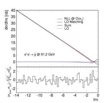
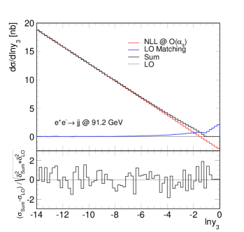
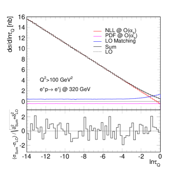
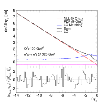
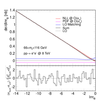
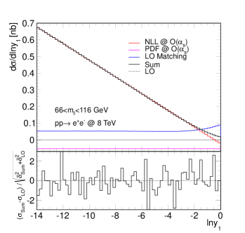
Figure 7: Test of the quasi-local matching procedure for hard processes with external quarks. Thrust (left panels) and leading jet rate (right panels) are compared between leading order and the first-order expanded resummed and matched prediction for $e^{+}e^{-}\to q\bar{q}$ (top), $e^{+}q\to e^{+}q$ (middle) and $q\bar{q}\to e^{+}e^{-}$ (bottom), all mediated by photon and $Z$-boson exchange.

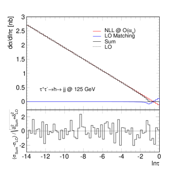
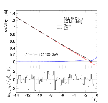
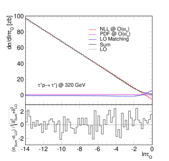
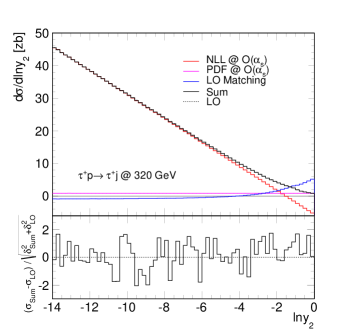
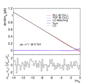
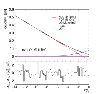
Figure 8: Test of the quasi-local matching procedure for hard processes with external gluons. Thrust (left panels) and leading jet rate (right panels) are compared between leading order and the first-order expanded resummed and matched prediction for $\tau^{+}\tau^{-}\to gg$ (top), $\tau^{+}g\to\tau^{+}g$ (middle) and $gg\to\tau^{+}\tau^{-}$ (bottom), all mediated by Higgs-boson exchange.

3.3 A proof of concept: transverse thrust

In order to demonstrate the completeness of our framework, we compute the resummed and matched distribution for a specific observable. We concentrate on the hadron-collider variant of the thrust observable, i.e. transverse thrust $T_{\perp}$. This global event-shape observable is defined as

$$T_{\perp}=\max_{\vec{n}_{\perp}}\frac{\sum_{i}|\vec{p}_{\perp i}\cdot\vec{n}_{\perp}|}{\sum_{i}p_{\perp i}},$$ (32)

where the sum runs over all final-state particles, with $\vec{p}_{\perp i}$ the particle’s momentum transverse to the beam direction, and $p_{\perp i}=|\vec{p}_{\perp i}|$. The maximimal $T_{\perp}$ is found by variation of the transverse unit vector $\vec{n}_{\perp}$. Transverse thrust has been studied by the Tevatron experiments [118, 119] and, more recently, also by the ATLAS [120] and CMS [121] collaborations. Perturbative calculations for this distribution exist at NLO [122] and also at the resummed level in the Caesar framework [47, *Banfi:2003je, *Banfi:2004nk, *Banfi:2004yd]. In particular, the event shape that vanishes at Born level is $\tau_{\perp}=1-T_{\perp}$. Details of the resummation for a generic global event shapes are given in App. B. The response of the observable in the presence of soft / collinear emissions (see Eq. (25)) is parametrized by the coefficients given in Table 1. Because the underlying Born processes is a $2\to 2$ QCD scattering, the color structure is non-trivial, hence we are able to put at work our construction of the soft function. In Figs. 9 and 10, we plot the transverse thrust distribution for $pp$ collisions at 8 TeV. We apply asymmetric cuts on the two leading jets, i.e. $p_{\perp 1}>100$ GeV, $p_{\perp 2}>80$ GeV and we set $\mu_{R}=\mu_{F}=H_{T}/2$, with $H_{T}=\sum_{i}p_{\perp i}$.

In particular, the plot in Fig. 9 is analogous to the ones already shown in Sec. 3.2 and it provides yet another check of our matching procedure: the sum of the explicit expansion of the resummation (red), the collinear counterterm (magenta) and the LO matching term (blue) is plotted in solid black and it has to be compared to the LO calculation (dotted black). The bottom panel shows that the difference between the two is zero, within the Monte Carlo uncertainty.

Finally, in Fig. 10 we plot the resummed and matched distribution for transverse thrust (black curve). For comparison, we also show the resummation on its own (red curve). We show two possible choices for the hard scale: $Q=\sqrt{s}$ (on the left) and $Q=H_{T}/2$ (on the right). The latter, more natural in hadron-hadron collisions, corresponds to a rescaling of the resummation coefficients in Table 1, namely $d_{l}\to d_{l}\left(H_{T}/2/\sqrt{s}\right)^{a}$.The key feature of this plot is that the soft function and matching are computed in a fully automated way at run-time, leading to NLL resummed and matched distributions with a similar level of automation as Monte Carlo event generators.

leg $l$	$a_{l}$	$b_{l}$	$d_{l}$	$g_{l}(\phi)$
$1$	$1$	$0$	$1/\sin\theta$	$1-|\cos\phi|$
$2$	$1$	$0$	$1/\sin\theta$	$1-|\cos\phi|$
$3$	$1$	$1$	$1/\sin^{2}\theta$	$\sin^{2}\phi$
$4$	$1$	$1$	$1/\sin^{2}\theta$	$\sin^{2}\phi$

Table 1: Coefficients of the Caesar formula that specify the NLL resummation of transverse thrust [47, *Banfi:2003je, *Banfi:2004nk, *Banfi:2004yd]. They correspond to the choice for the hard scale $Q=\sqrt{s}$; $\theta$ being the scattering angle in the partonic centre of mass frame, and $\phi$ denoting the azimuth.

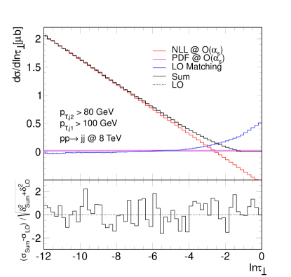
Figure 9: Test of the matching procedure for transverse thrust. The leading-order prediction is compared to the first-order expanded resummed and the LO matching term.

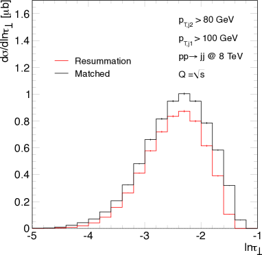
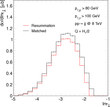
Figure 10: The transverse-thrust distribution for $pp$ collisions at 8 TeV, with asymmetric cuts $p_{\perp 1}>100$ GeV, $p_{\perp 2}>80$ GeV.

4 Conclusions and Outlook

Multi-jet physics is central in the physics program of the LHC. In this paper, we have overcome the two main technical difficulties that prevented NLL resummed calculations to be performed in processes with high jet multiplicity.

The first issue was related to the color structure of soft emissions at wide angle, i.e. away from the jets, the complexity of which rapidly increases with the number of hard jets. We have solved this problem by constructing and implementing a framework in which the NLL soft function is computed in an highly automated way. The algorithm constructs an appropriate color basis for the partonic process at hand, and evaluates color operators and the decomposition of Born amplitudes in this basis. It makes use of the matrix-element generator Comix to access the color-ordered partial amplitudes that are needed for the evaluation of the soft function. Using this framework, we have obtained and validated results for the soft function for all QCD processes with up to five hard jets in the final state, i.e. $2\to 5$ QCD amplitudes, and we have studied the validity of the widely used large $N_{C}$ approximation. We have found that the impact of finite-$N_{C}$ corrections is significant, especially for processes with many gluons.

We have tackled the second problem of matching resummed predictions to fixed-order calculations. In the traditional way of addressing this problem, one matches the resummed distribution of a given observable $v$ to the one obtained at fixed-order (typically NLO). The main drawback of this approach is that the fixed-order result and the expanded resummed result have to be computed independently in extreme regions of phase space, i.e. at very small $v$, where numerical cancellation is hard to achieve. We improve upon this situation by introducing a quasi-local matching scheme at leading order, which generates the finite remainder directly. As a proof of concept, we computed within our framework the NLL transverse-thrust distribution matched to LO. Although in this study we have mainly concentrated on global event shapes, our framework can be easily extended to the case of non-global observables.

We see this rather technical paper as the first necessary step in a rich program aimed at the phenomenological applications of resummed perturbation theory in multi-jet physics. Moreover, because we implement resummed calculations in the Sherpa framework, we have the possibility of making precise comparisons between analytic resummation and Monte-Carlo parton showers. This will provide insights on the benefits and limitations of both approaches and perhaps even indicate ways to improve the formal accuracy of the parton shower.

Appendix A Over-complete color bases

Color bases constructed from irreducible QCD representations do not meet our requirement 1 of the list in Sec. 2.1. Although we do not automate the construction of orthonormal bases this for work, we do employ their generic properties in several arguments throughout this section. For a complete approach to their construction see [97].

We define an orthogonal basis element $e_{\alpha}$ so that

$$\langle e_{\beta}|e_{\alpha}\rangle=e_{\beta\alpha}=\lambda_{\alpha}\delta_{\beta\alpha}\,,\qquad\text{(no sum on $\alpha$)}\,$$ (33)

where $\lambda_{\alpha}$ is the weight of the representation. For a given physical process, the dimensionality of the orthogonal $e$-basis may differ from the $c$-basis, in which case the indices in Eq. (8) versus Eq. (33) also differ. Starting with the metric $e_{\alpha\beta}$, we define the (possibly non-square) transformation to the $c$-basis via

$$R:\to R^{\;\;\alpha^{\prime}}_{\alpha}e_{\alpha^{\prime}\beta^{\prime}}(R^{T})^{\beta^{\prime}}_{\;\;\beta} = \;c_{\alpha\beta}\qquad R_{\;\;\alpha^{\prime}}^{\alpha}e^{\alpha^{\prime}\beta^{\prime}}(R^{T})_{\beta^{\prime}}^{\;\;\beta} = \;c^{\alpha\beta}.$$ (34)

As both $c_{\alpha\beta}$ and $c^{\alpha\beta}$ are symmetric, their (independent) eigenvectors correspond to the row elements of $R$ providing a straight-forward construction.

A.1 General proofs for the $N_{C}=3+\epsilon$ expansion

Lemma 1

Assuming $N_{C}=3+\epsilon$, with $\epsilon>0$ and $\epsilon\ll 1$, we can cleanly separate the finite part of the inverse metric from the divergent one, i.e.

$$c^{\alpha\beta}|_{N_{C}=3+\epsilon}=\frac{1}{\epsilon}\tilde{c}^{\,\alpha\beta}+c^{\alpha\beta}_{R}|_{N_{C}=3}+{\cal O}(\epsilon),$$ (35)

where $c^{\alpha\beta}_{R}$ and $\tilde{c}^{\,\alpha\beta}$ are regular at $N_{C}=3$.

Proof

For general $N_{C}$, the metric can be brought to diagonal form where the $\lambda_{\alpha}$ are polynomial in $N_{C}$ corresponding to the weights of irreducible representations, which in the limit $\epsilon\to 0$ are either ${\mathcal{O}}{(1)}$ or ${\mathcal{O}}{(\epsilon)}$. In the latter case, let us parameterize such eigenvalues as $\lambda_{0}=\kappa\epsilon$ where $\kappa$ is a constant.

The inverse of the orthogonal metric is a matrix with diagonal entries $1/\lambda_{\alpha}$. We construct the tensor $\tilde{c}^{\,\alpha\beta}$ by rotating only the $1/\lambda_{0}$ components back to the $c$-basis. Defining $\alpha^{\prime}_{0}$ as the indices running over the vanishing weights we have

$$\tilde{c}^{\,\alpha\beta}=\kappa\,R^{\alpha}_{\;\;\alpha^{\prime}_{0}}\delta^{\alpha_{0}^{\prime}\beta^{\prime}}\left(R^{T}\right)^{\;\;\beta}_{\beta^{\prime}}.$$ (36)

Lemma 2

All color products ${\bf T}_{i}\,\cdot\,{\bf T}_{j}$ belong to the null space of the singular part of the inverse metric, i.e.

$$\tilde{c}^{\,\alpha\beta}({\bf T}_{i}\,\cdot\,{\bf T}_{j})_{\beta\gamma}={\mathbf{0}}^{\alpha}_{\;\;\gamma}\,.$$ (37)

Corollary

An interesting, and computationally advantageous, consequence of the above Lemma is that in order to obtain

$$\mathcal{S}(\xi)_{N_{C}=3+\epsilon}=\mathcal{S}(\xi)_{N_{C}=3}+{\mathcal{O}}{(\epsilon)}\,.$$ (38)

we only have to evaluate the color metric and its inverse with $N_{C}=3+\epsilon$, while computing all color producs ${\bf T}_{i}\,\cdot\,{\bf T}_{j}$ at $N_{C}=3$. Therefore, the inversion of the metric at $N_{C}=3+\epsilon$ (with $\epsilon$ small) provides a valid alternative to dimensional reduction for computing the soft function.

Proof

Rotating $\tilde{c}^{\;\alpha\beta}$ to the e-basis we define an element

$$\langle e_{\alpha}|=\langle c_{\alpha^{\prime}}|R^{\alpha^{\prime}}_{\;\;\alpha}\,,$$ (39)

so that for every $0$ eigenvalue of $c_{\alpha\beta}$ there is a corresponding element $\langle e_{\alpha_{0}}|$ in the orthogonal basis which satisfies

$$\langle e_{\alpha_{0}}|e_{\beta}\rangle=0\quad\forall\beta\,.$$ (40)

Since ${\bf T}_{i}\,\cdot\,{\bf T}_{j}|e_{\beta}\rangle$ is a coefficient times an element of the orthogonal basis, we conclude that $({\bf T}_{i}\cdot{\bf T}_{j})_{\alpha_{0}\beta}=0$. Repeating the argument and noting that $c^{\alpha\beta}$ is symmetric, we conclude that the corresponding rows and columns of $({\bf T}_{i}\cdot{\bf T}_{j})$ are zero. In the $e$-basis we clearly have

$$\delta^{\alpha\alpha_{0}}\langle e_{\alpha_{0}}|\,{\bf T}_{i}\cdot{\bf T}_{j}\,|e_{\gamma}\rangle\;\Rightarrow\;\tilde{c}^{\,\alpha\beta}({\bf T}_{i}\cdot{\bf T}_{j})_{\beta\gamma}={\mathbf{0}}^{\alpha}_{\;\;\gamma}\,,$$ (41)

which gives the desired result.

In order to demonstrate the corollary we evaluate all color products at $N_{C}=3+\epsilon$ and we then write the soft anomalous dimension Eq. (2) at small $\epsilon$ as

$$\Gamma_{\alpha\beta}|_{N_{C}=3+\epsilon}=\Gamma_{\alpha\beta}|_{N_{C}=3}+\epsilon\,\tilde{\Gamma}_{\alpha\beta}|_{N_{C}=3}\,.$$ (42)

The first term contributing to the soft function $\mathcal{S}$ which involves the inverse metric comes from expanding the exponential to second order

$$\mathcal{S}(\xi)\sim\frac{\xi^{2}}{2!}\left[\Gamma_{\beta\alpha}+\epsilon\,\tilde{\Gamma}_{\beta\alpha}\right]\left[c^{\alpha\gamma}_{R}+\frac{1}{\epsilon}\tilde{c}^{\,\alpha\gamma}\right]\left[\Gamma_{\gamma\alpha^{\prime}}+\epsilon\,\tilde{\Gamma}_{\gamma\alpha^{\prime}}\right].$$ (43)

Using (37) on all the color products that enter the definition of $\Gamma$, one finds no finite terms originating from the interference of the $1/\epsilon$ pole of the inverse metric and the ${\mathcal{O}}{(\epsilon)}$ contribution to the anomalous dimensions. Furthermore, this holds for higher terms in the expansion of the exponential. Therefore, all the color products necessary to construct the soft anomalous dimension can be safely computed at $N_{C}=3$, while it is still necessary to compute the metric and its inverse at $N_{C}=3+\epsilon$

Finally, we note that using $N_{C}=3+\epsilon$ to invert the metric involves a large cancellation among the entries of $c^{\alpha\beta}$. However, the convergence is better than expected since the coefficients of $1/\epsilon$ are roughly proportional to the number of corresponding ${\bf 0}$-representations, which is smaller than the total number of irreducible representations for a given process.

A.2 A concrete example: $gg\to gg$

We list here several different manifestations of the 4-gluon basis as specific examples for our more general discussion in the text.

Trace basis

Let us consider the trace basis for this process:

$$c_{1} =K_{c}({\bf t}_{a_{1}}{\bf t}_{a_{2}}{\bf t}_{a_{3}}{\bf t}_{a_{4}}+{\bf t}_{a_{1}}{\bf t}_{a_{4}}{\bf t}_{a_{3}}{\bf t}_{a_{2}}),\qquad c_{4} =K_{d}\delta_{a_{1}a_{2}}\delta_{a_{3}a_{4}},$$

$$c_{2} =K_{c}({\bf t}_{a_{1}}{\bf t}_{a_{2}}{\bf t}_{a_{4}}{\bf t}_{a_{3}}+{\bf t}_{a_{1}}{\bf t}_{a_{3}}{\bf t}_{a_{4}}{\bf t}_{a_{2}}),\qquad c_{5} =K_{d}\delta_{a_{1}a_{3}}\delta_{a_{2}a_{4}},$$

$$c_{3} =K_{c}({\bf t}_{a_{1}}{\bf t}_{a_{3}}{\bf t}_{a_{2}}{\bf t}_{a_{4}}+{\bf t}_{a_{1}}{\bf t}_{a_{4}}{\bf t}_{a_{2}}{\bf t}_{a_{3}}),\qquad c_{6} =K_{d}\delta_{a_{1}a_{4}}\delta_{a_{2}a_{3}},$$ (44)

where ${\bf t}_{a_{i}}$ are the color generators in the fundamental representation and a trace over their fundamental-representation indices is implicit. Note that $K_{c}=N_{C}(16N_{C}^{6}-3N_{C}^{4}+16N_{C}^{2}-6)^{-\frac{1}{2}}$ and $K_{d}=(N_{C}^{2}-1)^{-1}$, so that the basis is normalized. The tree-level partial amplitude coefficients corresponding to these color basis elements are

$$c_{1}\to m_{0}(1,2,3,4),\quad c_{2}\to m_{0}(1,2,4,3),\quad c_{3}\to m_{0}(1,4,2,3),\quad c_{4}=c_{5}=c_{6}=0.$$ (45)

Dimensionally reduced trace basis

The basis in Eq. (A.2) is over-complete and consequently the color metric is not invertible for $N_{C}=3$. However, if we consider a reduced basis, obtained by taking

$$c^{\prime}_{1} =c_{1},\qquad c^{\prime}_{2} =c_{2},\qquad c^{\prime}_{3} =c_{3},\qquad c^{\prime}_{4} =\frac{K_{d}^{\prime}}{K_{d}}(c_{4}+c_{6}),\qquad c^{\prime}_{5} =\frac{K_{d}^{\prime}}{K_{d}}(c_{5}+c_{6}),$$ (46)

where $K_{d}^{\prime}=1/\sqrt{2N_{C}^{2}(N_{C}^{2}-1)}$, the metric is then invertible for $N_{C}=3$, the connected components remain synced with the hard matrix (45), and the resulting $\mathcal{S}(N_{C}=3)$ is unchanged.

Adjoint basis

We can now write the 5-dimensional $f$-basis

$$c_{1} =K_{a}f^{a_{1}a_{4}e_{1}}f^{e_{1}a_{3}a_{2}},\qquad c_{2}=K_{a}f^{a_{1}a_{3}e_{1}}f^{e_{1}a_{4}a_{2}},$$

$$c_{3} =K_{d}\delta_{a_{1}a_{4}}\delta_{a_{2}a_{3}}, c_{4}=K_{d}\delta_{a_{1}a_{2}}\delta_{a_{3}a_{4}},\qquad c_{5}=K_{d}\delta_{a_{1}a_{3}}\delta_{a_{2}a_{4}},$$ (47)

where $K_{a}=(4N_{C}^{2}(N_{C}^{2}-1))^{-\frac{1}{2}}$ and $K_{d}=(N_{C}^{2}-1)^{-1}$. We can make connection to the trace basis by repeated application of the fundamental Lie algebra to see that

$$c_{1} =K_{a}\left[({\bf t}_{a_{1}}{\bf t}_{a_{2}}{\bf t}_{a_{4}}{\bf t}_{a_{3}}+{\bf t}_{a_{1}}{\bf t}_{a_{3}}{\bf t}_{a_{4}}{\bf t}_{a_{2}})-({\bf t}_{a_{1}}{\bf t}_{a_{2}}{\bf t}_{a_{3}}{\bf t}_{a_{4}}+{\bf t}_{a_{1}}{\bf t}_{a_{4}}{\bf t}_{a_{3}}{\bf t}_{a_{2}})\right],$$

$$c_{2} =K_{a}\left[({\bf t}_{a_{1}}{\bf t}_{a_{2}}{\bf t}_{a_{3}}{\bf t}_{a_{4}}+{\bf t}_{a_{1}}{\bf t}_{a_{4}}{\bf t}_{a_{3}}{\bf t}_{a_{2}})-({\bf t}_{a_{1}}{\bf t}_{a_{4}}{\bf t}_{a_{2}}{\bf t}_{a_{3}}+{\bf t}_{a_{1}}{\bf t}_{a_{3}}{\bf t}_{a_{2}}{\bf t}_{a_{4}})\right].$$ (48)

in terms of fundamental representation generators. The hard coefficients are the same partial ordered amplitudes though we now have multi-peripheral labelling

$$c_{1}\to m_{0}(1,3,4,2),\quad c_{2}\to m_{0}(1,4,3,2),\quad c_{3}=c_{4}=c_{5}=0.$$ (49)

The evaluation of $\mathcal{S}(\xi)$ in the adjoint basis is equivalent to the trace basis at $N_{C}=3$.

Inversion with $N_{C}=3+\epsilon$

We consider here the trace basis for $N_{C}=3+\epsilon$. We note that there are no additional null eigenvalues for $N_{C}\neq 3$. We then take the $\epsilon\to 0$ limit and expand the matrix representing the color metric in terms of its regular and singular pieces, as in Eq. (35). The residue of the $1/\epsilon$ pole is

$$\tilde{c}^{\alpha\beta}\;=\;\left(\begin{array}[]{ccc}K_{3\times 3}(\frac{23}{27})&K_{3\times 3}(\sqrt{\frac{92}{243}})\\ K_{3\times 3}(\sqrt{\frac{92}{243}})&K_{3\times 3}(\frac{4}{9})\\ \end{array}\right),$$ (52)

where $K_{3\times 3}(a)$ is a $3\times 3$ matrix with each element equal to $a$. The matrix in Eq. (52) is precisely the trace-basis form for the inverse eigenvalue $\lambda_{0}\sim 1/\epsilon$ of the $N_{C}=3$ $0$-representation in the orthogonal basis. One can verify that the matrix $({\bf T}_{i}\cdot{\bf T}_{j})_{\alpha\beta}$ at $N_{C}=3$ for all $i$ and $j$ is in the null space of $\tilde{c}^{\alpha\beta}$. This a concrete manifestation of the behavior expected from the discussion in App. A.1.

A.3 Bases properties for multi-parton processes

In Tables 2 and 3 we summarize the main properties of the multi-parton processes considered in Sec. 2.

Sub-process	$gggg$	$q\bar{q}gg$	$q\bar{q}q\bar{q}$	$ggggg$	$q\bar{q}ggg$	$q\bar{q}q\bar{q}g$
Dim. basis	5	3	2	16	10	4
Dim. Born	2	2	2	6	6	4
zero eigenvalues	0	0	0	0	0	0

Table 2: Summary of basis properties for all $4$- and $5$-parton processes. Pure gluon processes are listed in the adjoint $f$-basis.

Sub-process	$6g$	$q\bar{q}4g$	$q\bar{q}q\bar{q}gg$	$qqqq\bar{q}q$	$7g$	$q\bar{q}5g$	$q\bar{q}q\bar{q}3g$	$q\bar{q}q\bar{q}q\bar{q}g$
Dim. basis	79	46	14	6	421	252	62	18
Dim. Born	24	24	12	6	120	120	48	18
zero eigenvalues	5	6	1	0	70	75	12	1

Table 3: Summary of basis properties for all $6$- and $7$-parton processes. Pure gluon processes are listed in the adjoint $f$-basis.

Appendix B The Caesar framework

Caesar  [47, *Banfi:2003je, *Banfi:2004nk, *Banfi:2004yd] is a computer program that allows one to perform the resummation of a large class of observables, namely global event shapes, to NLL accuracy. In this appendix we recap, without re-deriving them, the expressions of the leading and next-to-leading function $g_{1}^{(\delta)}$ and $g_{2}^{(\delta,\mathcal{B})}$ in Eq. (3.1) as obtained in the Caesar framework. The LL function reads

$$g_{1}^{(\delta)}(\alpha_{\rm S}L) =$$

$$-\sum_{l=1}^{n}\frac{C_{l}}{2\pi\beta_{0}\lambda b_{l}}\left[(a-2\lambda)\ln\left(1-\frac{2\lambda}{a}\right)-(a+b_{l}-2\lambda)\ln\left(1-\frac{2\lambda}{a+b_{l}}\right)\right],$$ (53)

where $\lambda=\alpha_{\rm S}\beta_{0}L$, $\alpha_{\rm S}=\alpha_{\rm S}(\mu_{R}^{2})$ and $\beta_{0}$ is the one-loop coefficient of the QCD $\beta$-function, $\beta(\alpha_{\rm S})=-\alpha_{\rm S}\left(\alpha_{\rm S}\beta_{0}+\alpha_{\rm S}^{2}\,\beta_{1}+\dots\right)$, with

$$\beta_{0}=\frac{11C_{A}-2n_{f}}{12\pi},\quad\beta_{1}=\frac{17C_{A}^{2}-5C_{A}n_{f}-3C_{F}n_{f}}{24\pi^{2}}.$$ (54)

The result in Eq. (B) consists of a sum over all the hard partons and the dependence on the color is trivial and only enters through the Casimir of each leg $l$, ($C_{F}$ for a quark leg, $C_{A}$ for a gluon leg). Note also that $a_{1}=a_{2}=\dots=a_{n}=a>0$.

The result for the NLL function $g_{2}^{(\delta,\mathcal{B})}$ has a richer structure:

$$g_{2}^{(\delta,\mathcal{B})}(\alpha_{\rm S}L) =-\sum_{l=1}^{n}C_{l}\left[\frac{r^{(2)}_{l}}{b_{l}}+B_{l}\,T\left(\frac{L}{a+b_{l}}\right)\right]+\partial_{L}\left[Lg_{1}^{(\delta)}(\alpha_{\rm S}L)\right]\left(\ln\bar{d}_{l}-b_{l}\ln\frac{2E_{l}}{Q}\right)$$

$$+\sum_{l=1}^{n_{\text{initial}}}\ln\frac{q^{(l)}(x_{l},\mu_{F}^{2}e^{-\frac{2L}{a+b_{l}}})}{q^{(l)}(x_{l},\mu_{F}^{2})}+\ln\mathcal{F}\left(\partial_{L}Lg_{1}^{(\delta)}(\alpha_{\rm S}L)\right)$$

$$-T\left(L/a\right)\sum_{l=1}^{n}C_{l}\ln\frac{Q_{12}}{Q}+\ln\mathcal{S}\left(T\left(L/a\right)\right).$$ (55)

The first term in the square brackets in Eq. (B) contains the two-loop contributions to the DGLAP splitting function in the soft limit and to the QCD $\beta$-function, as well as the dependence on the renormalization scale $\mu_{R}$:

$$r_{l}^{(2)} =\left(\frac{K}{4\pi^{2}\beta_{0}^{2}}-\frac{1}{2\pi\beta_{0}}\ln\frac{\mu_{R}^{2}}{Q^{2}}\right)\left[\left(a+b_{l}\right)\ln\left(1-\frac{2\lambda}{a+b_{l}}\right)-a\ln\left(1-\frac{2\lambda}{a}\right)\right]$$

$$+\frac{\beta_{1}}{2\pi\beta_{0}^{3}}\left[\frac{a}{2}\ln^{2}\left(1-\frac{2\lambda}{a}\right)-\frac{a+b_{l}}{2}\ln^{2}\left(1-\frac{2\lambda}{a+b_{l}}\right)+a\ln\left(1-\frac{2\lambda}{a}\right)\right.$$

$$\left.-(a+b_{l})\ln\left(1-\frac{2\lambda}{a+b_{l}}\right)\right],\quad\text{with}\quad K=C_{A}\left(\frac{67}{18}-\frac{\pi^{2}}{6}\right)-\frac{5}{9}n_{f}.$$ (56)

The second term in the square brackets instead captures hard collinear emissions to a quark leg ($B_{q}=-\frac{3}{4}$) or to a gluon leg ($B_{g}=-\pi\beta_{0}$); we have introduced

$$T(L)=\frac{1}{\pi\beta_{0}}\ln\frac{1}{1-2\alpha_{s}\beta_{0}L}$$ (57)

The last term of the first line of Eq. (B) contains

$$\ln\bar{d}_{l}=\ln d_{l}+\int_{0}^{2\pi}\frac{d\phi}{2\pi}\ln g_{l}(\phi),$$ (58)

while $E_{l}$ is the energy of leg $l$. We note that the contribution in this round brackets is actually frame-independent. We move then to the second line of Eq. (B) and the first term we encounter is the one that depends on the PDFs ($\mu_{F}$ is the factorization scale). This contribution comes about because we veto emissions collinear to the incoming legs which would contribute to the event shape more than a quantity $v$. There is then a term ($\mathcal{F}$) describing the effect of multiple emissions. The calculation of this term is highly non-trivial for generic observables and indeed this is one of the central aspects of the analysis of Refs. [47, *Banfi:2003je, *Banfi:2004nk, *Banfi:2004yd]. However, at NLL, multiple emissions have a color structure identical to $g_{1}^{(\delta)}$, thus this term is trivial from the point of view of our current analysis. For additive observables, like, for instance, transverse thrust considered in Sec. 3.3, this multiple-emission contribution has a rather simple form

$$\mathcal{F}(L)=\frac{e^{\gamma_{E}\partial_{L}\left(Lg_{1}^{(\delta)}(\alpha_{\rm S}L)\right)}}{\Gamma\left(1-\partial_{L}\left(Lg_{1}^{(\delta)}(\alpha_{\rm S}L)\right)\right)}.$$ (59)

Finally, in the last line we encounter the contributions due to soft radiation at large angle, which we can, for convenience, divide into a diagonal contribution and one with a non-trivial matrix structure.

Thus, all the terms but the last one in the Caesar master formula Eq. (B) are diagonal in color and therefore apply to processes with an arbitrary number of hard legs. The results of Sec. 2 provide an automated way of computing the only contribution at NLL with a non-trivial color structure, namely the soft function $\mathcal{S}$, which captures the effect of soft gluon emitted at wide angles.

References

- [1] ATLAS Collaboration Collaboration, G. Aad et al., Measurement of multi-jet cross sections in proton-proton collisions at a 7 TeV center-of-mass energy, Eur.Phys.J. C71 (2011) 1763, [arXiv:1107.2092]
- [2] ATLAS Collaboration Collaboration, G. Aad et al., Measurement of the production cross section of jets in association with a Z boson in pp collisions at sqrt(s) = 7 TeV with the ATLAS detector, arXiv:1304.7098
- [3] CMS Collaboration Collaboration, V. Khachatryan et al., Measurements of jet multiplicity and differential production cross sections of Z+jets events in proton-proton collisions at sqrt(s)=7 TeV, arXiv:1408.3104
- [4] M. L. Mangano, M. Moretti, F. Piccinini, R. Pittau, and A. D. Polosa, ALPGEN, a generator for hard multiparton processes in hadronic collisions, JHEP 07 (2003) 001, [hep-ph/0206293]
- [5] A. Cafarella, C. G. Papadopoulos, and M. Worek, Helac-Phegas: A generator for all parton level processes, Comput. Phys. Commun. 180 (2009) 1941–1955, [arXiv:0710.2427]
- [6] T. Gleisberg and S. Höche, Comix, a new matrix element generator, JHEP 12 (2008) 039, [arXiv:0808.3674]
- [7] A. Denner and S. Dittmaier, Reduction schemes for one-loop tensor integrals, Nucl. Phys. B734 (2006) 62–115, [hep-ph/0509141]
- [8] G. Ossola, C. G. Papadopoulos, and R. Pittau, Reducing full one-loop amplitudes to scalar integrals at the integrand level, Nucl. Phys. B763 (2007) 147–169, [hep-ph/0609007]
- [9] R. Ellis, W. Giele, and Z. Kunszt, A numerical unitarity formalism for evaluating one-loop amplitudes, JHEP 03 (2008) 003, [arXiv:0708.2398]
- [10] T. Binoth, J. P. Guillet, G. Heinrich, E. Pilon, and T. Reiter, Golem95: A numerical program to calculate one-loop tensor integrals with up to six external legs, Comput. Phys. Commun. 180 (2009) 2317–2330, [arXiv:0810.0992]
- [11] C. F. Berger, Z. Bern, L. J. Dixon, F. Febres-Cordero, D. Forde, H. Ita, D. A. Kosower, and D. Maître, Automated implementation of on-shell methods for one-loop amplitudes, Phys. Rev. D78 (2008) 036003, [arXiv:0803.4180]
- [12] G. Bevilacqua, M. Czakon, M. Garzelli, A. van Hameren, A. Kardos, et al., HELAC-NLO, Comput.Phys.Commun. 184 (2013) 986–997, [arXiv:1110.1499]
- [13] G. Cullen, N. Greiner, G. Heinrich, G. Luisoni, P. Mastrolia, G. Ossola, T. Reiter, and F. Tramontano, Automated One-Loop Calculations with GoSam, Eur.Phys.J. C72 (2012) 1889, [arXiv:1111.2034]
- [14] F. Cascioli, P. Maierhöfer, and S. Pozzorini, Scattering Amplitudes with Open Loops, Phys.Rev.Lett. 108 (2012) 111601, [arXiv:1111.5206]
- [15] V. Hirschi, R. Frederix, S. Frixione, M. V. Garzelli, F. Maltoni, and R. Pittau, Automation of one-loop QCD corrections, JHEP 05 (2011) 044, [arXiv:1103.0621]
- [16] S. Badger, B. Biedermann, P. Uwer, and V. Yundin, Numerical evaluation of virtual corrections to multi-jet production in massless QCD, Comput.Phys.Commun. 184 (2013) 1981–1998, [arXiv:1209.0100]
- [17] S. Actis, A. Denner, L. Hofer, A. Scharf, and S. Uccirati, Recursive generation of one-loop amplitudes in the Standard Model, JHEP 1304 (2013) 037, [arXiv:1211.6316]
- [18] H. Ita, Z. Bern, L. J. Dixon, F. Febres-Cordero, D. A. Kosower, and D. Maître, Precise Predictions for Z + 4 Jets at Hadron Colliders, Phys.Rev. D85 (2012) 031501, [arXiv:1108.2229]
- [19] Z. Bern, L. Dixon, F. Febres Cordero, S. Hoeche, H. Ita, et al., Next-to-Leading Order -Jet Production at the LHC, Phys.Rev. D88 (2013) 014025, [arXiv:1304.1253]
- [20] S. Badger, B. Biedermann, P. Uwer, and V. Yundin, Next-to-leading order QCD corrections to five jet production at the LHC, Phys.Rev. D89 (2013) 034019, [arXiv:1309.6585]
- [21] G. Cullen, H. van Deurzen, N. Greiner, G. Luisoni, P. Mastrolia, et al., NLO QCD corrections to Higgs boson production plus three jets in gluon fusion, Phys.Rev.Lett. 111 (2013) 131801, [arXiv:1307.4737]
- [22] G. Marchesini and B. R. Webber, Simulation of QCD Jets Including Soft Gluon Interference, Nucl. Phys. B238 (1984) 1
- [23] T. Sjöstrand, A model for initial state parton showers, Phys. Lett. B157 (1985) 321
- [24] G. Marchesini and B. R. Webber, Monte Carlo Simulation of General Hard Processes with Coherent QCD Radiation, Nucl. Phys. B310 (1988) 461
- [25] Z. Nagy and D. E. Soper, A new parton shower algorithm: Shower evolution, matching at leading and next-to-leading order level, hep-ph/0601021
- [26] W. T. Giele, D. A. Kosower, and P. Z. Skands, A Simple shower and matching algorithm, Phys. Rev. D78 (2008) 014026, [arXiv:0707.3652]
- [27] S. Schumann and F. Krauss, A parton shower algorithm based on Catani-Seymour dipole factorisation, JHEP 03 (2008) 038, [arXiv:0709.1027]
- [28] S. Plätzer and S. Gieseke, Coherent Parton Showers with Local Recoils, JHEP 01 (2011) 024, [arXiv:0909.5593]
- [29] S. Plätzer and M. Sjödahl, Subleading improved Parton Showers, JHEP 07 (2012) 042, [arXiv:1201.0260]
- [30] Z. Nagy and D. E. Soper, Parton shower evolution with subleading color, JHEP 1206 (2012) 044, [arXiv:1202.4496]
- [31] S. Catani, F. Krauss, R. Kuhn, and B. R. Webber, QCD matrix elements + parton showers, JHEP 11 (2001) 063, [hep-ph/0109231]
- [32] M. L. Mangano, M. Moretti, and R. Pittau, Multijet matrix elements and shower evolution in hadronic collisions: -jets as a case study, Nucl. Phys. B632 (2002) 343–362, [hep-ph/0108069]
- [33] L. Lönnblad, Correcting the colour-dipole cascade model with fixed order matrix elements, JHEP 05 (2002) 046, [hep-ph/0112284]
- [34] F. Krauss, Matrix elements and parton showers in hadronic interactions, JHEP 08 (2002) 015, [hep-ph/0205283]
- [35] S. Frixione and B. R. Webber, Matching NLO QCD computations and parton shower simulations, JHEP 06 (2002) 029, [hep-ph/0204244]
- [36] P. Nason, A new method for combining NLO QCD with shower Monte Carlo algorithms, JHEP 11 (2004) 040, [hep-ph/0409146]
- [37] S. Frixione, P. Nason, and C. Oleari, Matching NLO QCD computations with parton shower simulations: the POWHEG method, JHEP 11 (2007) 070, [arXiv:0709.2092]
- [38] S. Höche, F. Krauss, M. Schönherr, and F. Siegert, QCD matrix elements + parton showers: The NLO case, JHEP 04 (2013) 027, [arXiv:1207.5030]
- [39] R. Frederix and S. Frixione, Merging meets matching in MC@NLO, JHEP 12 (2012) 061, [arXiv:1209.6215]
- [40] L. Lönnblad and S. Prestel, Merging Multi-leg NLO Matrix Elements with Parton Showers, JHEP 03 (2013) 166, [arXiv:1211.7278]
- [41] K. Hamilton, P. Nason, C. Oleari, and G. Zanderighi, Merging H/W/Z + 0 and 1 jet at NLO with no merging scale: a path to parton shower + NNLO matching, JHEP 05 (2013) 082, [arXiv:1212.4504]
- [42] K. Hamilton, P. Nason, E. Re, and G. Zanderighi, NNLOPS simulation of Higgs boson production, JHEP 10 (2013) 222, [arXiv:1309.0017]
- [43] S. Höche, Y. Li, and S. Prestel, Drell-Yan lepton pair production at NNLO QCD with parton showers, arXiv:1405.3607
- [44] J. R. Andersen and J. M. Smillie, Multiple Jets at the LHC with High Energy Jets, JHEP 06 (2011) 010, [arXiv:1101.5394]
- [45] M. Dasgupta and G. P. Salam, Event shapes in e+ e- annihilation and deep inelastic scattering, J.Phys. G30 (2004) R143, [hep-ph/0312283]
- [46] A. Banfi, G. P. Salam, and G. Zanderighi, Phenomenology of event shapes at hadron colliders, JHEP 06 (2010) 038, [arXiv:1001.4082]
- [47] A. Banfi, G. Salam, and G. Zanderighi, Semi-numerical resummation of event shapes, JHEP 01 (2002) 018, [hep-ph/0112156]
- [48] A. Banfi, G. P. Salam, and G. Zanderighi, Generalized resummation of QCD final state observables, Phys.Lett. B584 (2004) 298–305, [hep-ph/0304148]
- [49] A. Banfi, G. P. Salam, and G. Zanderighi, Resummed event shapes at hadron - hadron colliders, JHEP 08 (2004) 062, [hep-ph/0407287]. Erratum added online, nov/29/2004
- [50] A. Banfi, G. P. Salam, and G. Zanderighi, Principles of general final-state resummation and automated implementation, JHEP 03 (2005) 073, [hep-ph/0407286]
- [51] R. Abbate, M. Fickinger, A. H. Hoang, V. Mateu, and I. W. Stewart, Thrust at with Power Corrections and a Precision Global Fit for alphas(mZ), Phys.Rev. D83 (2011) 074021, [arXiv:1006.3080]
- [52] A. H. Hoang, D. W. Kolodrubetz, V. Mateu, and I. W. Stewart, C-parameter Distribution at N3LL′ including Power Corrections, arXiv:1411.6633
- [53] G. Oderda and G. F. Sterman, Energy and color flow in dijet rapidity gaps, Phys.Rev.Lett. 81 (1998) 3591–3594, [hep-ph/9806530]
- [54] R. Appleby and M. Seymour, The Resummation of interjet energy flow for gaps between jets processes at HERA, JHEP 0309 (2003) 056, [hep-ph/0308086]
- [55] J. R. Forshaw, A. Kyrieleis, and M. Seymour, Super-leading logarithms in non-global observables in QCD, JHEP 0608 (2006) 059, [hep-ph/0604094]
- [56] J. Forshaw, A. Kyrieleis, and M. Seymour, Super-leading logarithms in non-global observables in QCD: Colour basis independent calculation, JHEP 0809 (2008) 128, [arXiv:0808.1269]
- [57] J. Forshaw, J. Keates, and S. Marzani, Jet vetoing at the LHC, JHEP 0907 (2009) 023, [arXiv:0905.1350]
- [58] R. M. Duran Delgado, J. R. Forshaw, S. Marzani, and M. H. Seymour, The dijet cross section with a jet veto, JHEP 1108 (2011) 157, [arXiv:1107.2084]
- [59] X. Liu and F. Petriello, Resummation of jet-veto logarithms in hadronic processes containing jets, Phys.Rev. D87 (2013) 014018, [arXiv:1210.1906]
- [60] ATLAS Collaboration, G. Aad et al., Measurement of dijet production with a veto on additional central jet activity in pp collisions at =7 TeV using the ATLAS detector, arXiv:1107.1641
- [61] ATLAS Collaboration Collaboration, G. Aad et al., Measurement of production with a veto on additional central jet activity in pp collisions at sqrt(s) = 7 TeV using the ATLAS detector, Eur.Phys.J. C72 (2012) 2043, [arXiv:1203.5015]
- [62] ATLAS Collaboration Collaboration, G. Aad et al., Measurements of jet vetoes and azimuthal decorrelations in dijet events produced in collisions at = 7 TeV using the ATLAS detector, Eur.Phys.J. C74 (2014), no. 11 3117, [arXiv:1407.5756]
- [63] CMS Collaboration Collaboration, S. Chatrchyan et al., Measurement of the inclusive production cross sections for forward jets and for dijet events with one forward and one central jet in pp collisions at sqrt(s) = 7 TeV, JHEP 06 (2012) 036, [arXiv:1202.0704]
- [64] A. Banfi, G. P. Salam, and G. Zanderighi, NLL+NNLO predictions for jet-veto efficiencies in Higgs-boson and Drell-Yan production, JHEP 06 (2012) 159, [arXiv:1203.5773]
- [65] A. Banfi, P. F. Monni, G. P. Salam, and G. Zanderighi, Higgs and Z-boson production with a jet veto, Phys.Rev.Lett. 109 (2012) 202001, [arXiv:1206.4998]
- [66] A. Banfi, P. F. Monni, and G. Zanderighi, Quark masses in Higgs production with a jet veto, JHEP 1401 (2014) 097, [arXiv:1308.4634]
- [67] T. Becher and M. Neubert, Factorization and NNLL Resummation for Higgs Production with a Jet Veto, JHEP 07 (2012) 108, [arXiv:1205.3806]
- [68] T. Becher, M. Neubert, and L. Rothen, Factorization and +NNLO predictions for the Higgs cross section with a jet veto, JHEP 10 (2013) 125, [arXiv:1307.0025]
- [69] I. W. Stewart, F. J. Tackmann, J. R. Walsh, and S. Zuberi, Jet Resummation in Higgs Production at NNLL’+NNLO, Phys.Rev. D89 (2014) 054001, [arXiv:1307.1808]
- [70] R. Boughezal, X. Liu, F. Petriello, F. J. Tackmann, and J. R. Walsh, Combining Resummed Higgs Predictions Across Jet Bins, Phys.Rev. D89 (2014) 074044, [arXiv:1312.4535]
- [71] H.-N. Li, Z. Li, and C.-P. Yuan, QCD resummation for light-particle jets, Phys.Rev. D87 (2013) 074025, [arXiv:1206.1344]
- [72] M. Dasgupta, K. Khelifa-Kerfa, S. Marzani, and M. Spannowsky, On jet mass distributions in Z+jet and dijet processes at the LHC, JHEP 1210 (2012) 126, [arXiv:1207.1640]
- [73] Y.-T. Chien, R. Kelley, M. D. Schwartz, and H. X. Zhu, Resummation of Jet Mass at Hadron Colliders, Phys.Rev. D87 (2013) 014010, [arXiv:1208.0010]
- [74] T. T. Jouttenus, I. W. Stewart, F. J. Tackmann, and W. J. Waalewijn, Jet mass spectra in Higgs boson plus one jet at next-to-next-to-leading logarithmic order, Phys.Rev. D88 (2013) 054031, [arXiv:1302.0846]
- [75] A. J. Larkoski, G. P. Salam, and J. Thaler, Energy Correlation Functions for Jet Substructure, JHEP 1306 (2013) 108, [arXiv:1305.0007]
- [76] A. J. Larkoski and J. Thaler, Unsafe but Calculable: Ratios of Angularities in Perturbative QCD, JHEP 1309 (2013) 137, [arXiv:1307.1699]
- [77] A. J. Larkoski, D. Neill, and J. Thaler, Jet Shapes with the Broadening Axis, JHEP 1404 (2014) 017, [arXiv:1401.2158]
- [78] A. J. Larkoski, I. Moult, and D. Neill, Toward Multi-Differential Cross Sections: Measuring Two Angularities on a Single Jet, JHEP 1409 (2014) 046, [arXiv:1401.4458]
- [79] A. J. Larkoski, I. Moult, and D. Neill, Power Counting to Better Jet Observables, arXiv:1409.6298
- [80] E. Gerwick, S. Schumann, B. Gripaios, and B. Webber, QCD Jet Rates with the Inclusive Generalized kt Algorithms, JHEP 1304 (2013) 089, [arXiv:1212.5235]
- [81] M. Dasgupta, A. Fregoso, S. Marzani, and G. P. Salam, Towards an understanding of jet substructure, JHEP 1309 (2013) 029, [arXiv:1307.0007]
- [82] M. Dasgupta, A. Fregoso, S. Marzani, and A. Powling, Jet substructure with analytical methods, Eur.Phys.J. C73 (2013), no. 11 2623, [arXiv:1307.0013]
- [83] A. J. Larkoski, S. Marzani, G. Soyez, and J. Thaler, Soft Drop, JHEP 1405 (2014) 146, [arXiv:1402.2657]
- [84] A. Broggio, A. Ferroglia, B. D. Pecjak, and Z. Zhang, NNLO hard functions in massless QCD, arXiv:1409.5294
- [85] P. Hinderer, F. Ringer, G. F. Sterman, and W. Vogelsang, Toward NNLL Threshold Resummation for Hadron Pair Production in Hadronic Collisions, arXiv:1411.3149
- [86] Y. Dokshitzer and G. Marchesini, Hadron collisions and the fifth form-factor, Phys.Lett. B631 (2005) 118–125, [hep-ph/0508130]
- [87] Y. Dokshitzer and G. Marchesini, Soft gluons at large angles in hadron collisions, JHEP 0601 (2006) 007, [hep-ph/0509078]
- [88] N. Kidonakis, G. Oderda, and G. F. Sterman, Evolution of color exchange in QCD hard scattering, Nucl.Phys. B531 (1998) 365–402, [hep-ph/9803241]
- [89] R. Bonciani, S. Catani, M. L. Mangano, and P. Nason, Sudakov resummation of multiparton QCD cross sections, Phys. Lett. B575 (2003) 268–278, [hep-ph/0307035]
- [90] S. Catani, M. Ciafaloni, and G. Marchesini, Non-cancelling infrared divergences in QCD coherent state, Nucl. Phys. B264 (1986) 588–620
- [91] S. Catani and M. H. Seymour, The Dipole Formalism for the Calculation of QCD Jet Cross Sections at Next-to-Leading Order, Phys. Lett. B378 (1996) 287–301, [hep-ph/9602277]
- [92] S. Catani and M. H. Seymour, A general algorithm for calculating jet cross sections in NLO QCD, Nucl. Phys. B485 (1997) 291–419, [hep-ph/9605323]
- [93] A. Bassetto, M. Ciafaloni, and G. Marchesini, Jet structure and infrared sensitive quantities in perturbative QCD, Phys. Rept. 100 (1983) 201–272
- [94] M. Sjödahl, Color evolution of 2 3 processes, JHEP 0812 (2008) 083, [arXiv:0807.0555]
- [95] M. Sjödahl, Color structure for soft gluon resummation: A General recipe, JHEP 0909 (2009) 087, [arXiv:0906.1121]
- [96] M. Sjödahl, ColorMath - A package for color summed calculations in SU(Nc), Eur.Phys.J. C73 (2013) 2310, [arXiv:1211.2099]
- [97] S. Keppeler and M. Sjödahl, Orthogonal multiplet bases in SU(Nc) color space, JHEP 1209 (2012) 124, [arXiv:1207.0609]
- [98] C. Duhr, S. Höche, and F. Maltoni, Color-dressed recursive relations for multi-parton amplitudes, JHEP 08 (2006) 062, [hep-ph/0607057]
- [99] T. Gleisberg, S. Höche, F. Krauss, A. Schälicke, S. Schumann, and J. Winter, Sherpa 1., a proof-of-concept version, JHEP 02 (2004) 056, [hep-ph/0311263]
- [100] T. Gleisberg, S. Höche, F. Krauss, M. Schönherr, S. Schumann, F. Siegert, and J. Winter, Event generation with Sherpa 1.1, JHEP 02 (2009) 007, [arXiv:0811.4622]
- [101] M. L. Mangano and S. J. Parke, Multiparton amplitudes in gauge theories, Phys. Rept. 200 (1991) 301–367, [hep-th/0509223]
- [102] V. del Duca, A. Frizzo, and F. Maltoni, Factorization of tree QCD amplitudes in the high-energy limit and in the collinear limit, Nucl. Phys. B568 (2000) 211–262, [hep-ph/9909464]
- [103] V. Del Duca, L. J. Dixon, and F. Maltoni, New color decompositions for gauge amplitudes at tree and loop level, Nucl. Phys. B571 (2000) 51–70, [hep-ph/9910563]
- [104] F. Maltoni, K. Paul, T. Stelzer, and S. Willenbrock, Color-flow decomposition of QCD amplitudes, Phys. Rev. D67 (2003) 014026, [hep-ph/0209271]
- [105] G. ’t Hooft, A Planar Diagram Theory for Strong Interactions, Nucl.Phys. B72 (1974) 461
- [106] A. Schofield and M. H. Seymour, Jet vetoing and Herwig++, JHEP 01 (2011) 078, [arXiv:1103.4811]
- [107] S. Plätzer, Summing Large- Towers in Colour Flow Evolution, Eur.Phys.J. C74 (2014) 2907, [arXiv:1312.2448]
- [108] A. Schofield, Simulation of colour evolution in qcd scattering processes, . PhD Thesis University of Manchester
- [109] R. Kleiss and H. Kuijf, Multi-gluon cross-sections and five jet production at hadron colliders, Nucl. Phys. B312 (1989) 616
- [110] S. Höche, F. Krauss, M. Schönherr, and F. Siegert, Automating the POWHEG method in Sherpa, JHEP 1104 (2011) 024, [arXiv:1008.5399]
- [111] M. Dasgupta and G. Salam, Resummation of nonglobal QCD observables, Phys.Lett. B512 (2001) 323–330, [hep-ph/0104277]
- [112] M. Dasgupta and G. P. Salam, Accounting for coherence in interjet E(t) flow: A Case study, JHEP 03 (2002) 017, [hep-ph/0203009]
- [113] M. Cacciari, G. P. Salam, and G. Soyez, The Anti-k(t) jet clustering algorithm, JHEP 04 (2008) 063, [arXiv:0802.1189]
- [114] A. Banfi, G. Marchesini, and G. Smye, Away from jet energy flow, JHEP 0208 (2002) 006, [hep-ph/0206076]
- [115] M. D. Schwartz and H. X. Zhu, Non-global Logarithms at 3 Loops, 4 Loops, 5 Loops and Beyond, Phys.Rev. D90 (2014) 065004, [arXiv:1403.4949]
- [116] Y. Hatta and T. Ueda, Resummation of non-global logarithms at finite , Nucl.Phys. B874 (2013) 808–820, [arXiv:1304.6930]
- [117] T. Gleisberg and F. Krauss, Automating dipole subtraction for QCD NLO calculations, Eur. Phys. J. C53 (2008) 501–523, [arXiv:0709.2881]
- [118] D0 Collaboration Collaboration, I. Bertram, Jet results at the D0 experiment, Acta Phys.Polon. B33 (2002) 3141–3146
- [119] CDF Collaboration Collaboration, T. Aaltonen et al., Measurement of Event Shapes in Proton-Antiproton Collisions at Center-of-Mass Energy 1.96 TeV, Phys.Rev. D83 (2011) 112007, [arXiv:1103.5143]
- [120] ATLAS Collaboration Collaboration, G. Aad et al., Measurement of event shapes at large momentum transfer with the ATLAS detector in collisions at TeV, Eur.Phys.J. C72 (2012) 2211, [arXiv:1206.2135]
- [121] CMS Collaboration Collaboration, V. Khachatryan et al., Study of hadronic event-shape variables in multijet final states in pp collisions at sqrt(s) = 7 TeV, JHEP 1410 (2014) 87, [arXiv:1407.2856]
- [122] Z. Nagy, Next-to-leading order calculation of three-jet observables in hadron-hadron collisions, Phys. Rev. D68 (2003) 094002, [hep-ph/0307268]