Consistency Relations for Large Field Inflation: Non-minimal Coupling

Abstract

We derive the consistency relations for a chaotic inflation model with a non-minimal coupling to gravity. For a quadratic potential in the limit of a small non-minimal coupling parameter $\xi$ and for a quartic potential without assuming small $\xi$, we give the consistency relations among the spectral index $n_{s}$, the tensor-to-scalar ratio $r$ and the running of the spectral index $\alpha$. We find that unlike $r$, $\alpha$ is less sensitive to $\xi$. If $r<0.1$, then $\xi$ is constrained to $\xi<0$ and $\alpha$ is predicted to be $\alpha\simeq-8\times 10^{-4}$ for a quartic potential. For a general monomial potential, $\alpha$ is constrained in the range $-2.7\times 10^{-3}<\alpha<-6\times 10^{-4}$ as long as $|\xi|\leq 10^{-3}$ if $r<0.1$.

I Introduction

In our previous paper, motivated by the possibility of a large tensor-to-scalar ratio $r$ bicep2 , we provided the consistency relations among the spectral index $n_{s}$, the tensor-to-scalar ratio $r$, and the running of the spectral index $\alpha$ for several large field inflation models (chaotic with monomial potential, natural, symmetry breaking) ck . The basic idea is to construct one relation out of two model parameters using three observables ($n_{s},r$, and $\alpha$). We find that $\alpha$ can be a discriminating probe of large field inflation models.

In this paper, we investigate the stability of the consistency relation for chaotic inflation with a monomial potential that we have recently found. To do this, we consider a non-minimal coupling as a ”perturber” of the model. Then, the number of model parameters becomes three and we need a fourth observable (for example, the ”running” of $\alpha$), but this would introduce complication and the comparison with the ”unperturbed” relation would be difficult. So, in this paper we fix one of the model parameters and examine how introducing the non-minimal coupling affects the relation.

II Consistency Relations for Chaotic Inflation with a Non-minimal Coupling

II.1 From Jordan to Einstein

We consider a single field inflation model with a non-minimal coupling to gravity. The action is given by

$$S=\int\sqrt{-g}\left(\frac{1}{16\pi G_{*}}\Omega(\phi)R-\frac{1}{2}(\nabla\phi)^{2}-V(\phi)\right)\,,$$ (1)

where $g_{\mu\nu}$ is the Jordan frame metric and $G_{*}$ is the bare gravitational constant and we shall set $8\pi G_{*}=1$ henceforth. As $\Omega(\phi)$ and $V(\phi)$, we take

$$\Omega(\phi)=1-\xi\phi^{2},\qquad V(\phi)=\frac{\lambda}{n}\phi^{n}\,,$$ (2)

where $\xi$ is a non-minimal coupling parameter. In our convention, $\xi=1/6$ corresponds to the conformal coupling.

As is well known, by introducing the new metric called Einstein frame metric $\widehat{g}_{\mu\nu}=\Omega g_{\mu\nu}$, the action can be rewritten as that of Einstein gravity with a scalar field fm :

$$S=\int\sqrt{-\widehat{g}}\left(\frac{1}{2}\widehat{R}-\frac{1}{2\Omega}\left(1+\frac{3\Omega_{,\phi}^{2}}{2\Omega}\right)(\widehat{\nabla}\phi)^{2}-\frac{V}{\Omega^{2}}\right)\,,$$ (3)

where the hatted variables are defined by $\widehat{g}_{\mu\nu}$ and $\Omega_{,\phi}=d\Omega/d\phi$. Hence in terms of the canonically normalized scalar field $\hat{\phi}$ defined by

$$d\hat{\phi}^{2}=\frac{1}{\Omega(\phi)}\left(1+\frac{3\Omega(\phi)_{,\phi}^{2}}{2\Omega(\phi)}\right)d\phi^{2}\equiv\frac{f(\phi)}{\Omega(\phi)}\,,$$ (4)

the system is reduced to the Einstein gravity plus a minimally coupled scalar field with the effective potential $\widehat{V}$ defined by

$$\widehat{V}=\frac{V}{\Omega^{2}}\,.$$ (5)

For $\Omega$ and $V$ in Eq. (2), $\widehat{V}$ with $n=4$ becomes flat for large $|\xi\phi^{2}|$ with $\xi<0$, which is the essence of the Higgs higgs (or Starobinsky alex ) inflation.

II.2 $r,n_{s}$, and $\alpha$

Hence, in order to compute the spectral index $n_{s}$, the tensor-to-scalar ratio $r$ and the running of the spectral index $\alpha$, we only need to calculate slow-roll parameters in terms of $\widehat{\phi}$ and $\widehat{V}$:

$$\widehat{\epsilon}\equiv\frac{1}{2}\left(\frac{\widehat{V}_{,\widehat{\phi}}}{\widehat{V}}\right)^{2},\quad\widehat{\eta}\equiv\frac{\widehat{V}_{,\widehat{\phi}\widehat{\phi}}}{\widehat{V}},\quad\widehat{\xi}\equiv\frac{\widehat{V}_{,\widehat{\phi}}\widehat{V}_{,\widehat{\phi}\widehat{\phi}\widehat{\phi}}}{\widehat{V}^{2}}\,.$$ (6)

Then $r,n_{s}$, and $\alpha$ are given by

$$r=16\widehat{\epsilon},\quad n_{s}-1=-6\widehat{\epsilon}+2\widehat{\eta},\quad\alpha=16\widehat{\epsilon}\widehat{\eta}-24\widehat{\epsilon}^{2}-2\widehat{\xi}$$ (7)

In fact, for a single scalar field, the observables are independent of the conformal transformation ms ; cy .

For example, in the limit of small $\xi$, the slow-roll parameters become

$$\widehat{\epsilon} = \frac{n^{2}}{2\phi^{2}}-\frac{1}{2}((n-8)n)\xi,$$ (8)

$$\widehat{\eta} = \frac{(n-1)n}{\phi^{2}}+(4-(n-8)n)\xi,$$ (9)

$$\widehat{\xi} = \frac{(n-2)(n-1)n^{2}}{\phi^{4}}+\frac{n(n((19-2n)n-14)+8)\xi}{\phi^{2}}+O(\xi^{2}\phi^{-2})\,,$$ (10)

and $r,n_{s}$, and $\alpha$ are given by

$$r = \frac{8n^{2}}{\phi^{2}}-8((n-8)n)\xi,$$ (11)

$$n_{s}-1 = -\frac{n(n+2)}{\phi^{2}}+((n-8)n+8)\xi,$$ (12)

$$\alpha = -\frac{2\left(n^{2}(n+2)\right)}{\phi^{4}}+\frac{2(n-4)n(n+2)\xi}{\phi^{2}}+16n\xi^{2}+O(\xi^{2}\phi^{-2})$$ (13)

On the other hand, for $n=4$ with large $|\xi|\phi^{2}$, we have

$$\widehat{\epsilon} = -\frac{8}{\left(1-6\xi\right)\xi\phi^{4}},$$ (14)

$$\widehat{\eta} = -\frac{8}{(1-6\xi)\phi^{2}}+\frac{4(12\xi-5)}{(1-6\xi)^{2}\xi\phi^{4}},$$ (15)

$$\widehat{\xi} = \frac{64}{(1-6\xi)^{2}\phi^{4}}+\frac{64(7-18\xi)}{(1-6\xi)^{3}\xi\phi^{6}},$$ (16)

and

$$r = -\frac{128}{(1-6\xi)\xi\phi^{4}},$$ (17)

$$n_{s}-1 = -\frac{16}{(1-6\xi)\phi^{2}}+\frac{8(1-24\xi)}{(1-6\xi)^{2}\xi\phi^{4}},$$ (18)

$$\alpha = -\frac{128}{(1-6\xi)^{2}\phi^{4}}+\frac{128(1-30\xi)}{(1-6\xi)^{3}\xi\phi^{6}}\,.$$ (19)

II.3 e-folding number

Finally, we provide the relation for the e-folding number until the end of inflation $N$. Since the scale factor and the proper time in the Jordan frame $a$ and $t$ are related to those in the Einstein frame $a=\Omega^{1/2}\widehat{a}$ and $dt=\Omega^{1/2}d\widehat{t}$, the Hubble parameter in the Jordan frame $H$ is related to that in the Einstein frame $\widehat{H}$ by the relation catena ; cy2

$$H=\frac{da/dt}{a}=\frac{1}{\Omega^{1/2}}\left(\widehat{H}+\frac{d\Omega/d\widehat{t}}{2\Omega}\right),$$ (20)

and the e-folding number $N$ is given by

$$N=\int^{t_{end}}Hdt=\int^{\widehat{t}_{end}}\widehat{H}d\widehat{t}+\frac{1}{2}\int_{\widehat{\phi}_{end}}\frac{\Omega_{,\widehat{\phi}}}{\Omega}d\widehat{\phi}\,.$$ (21)

Under the slow-roll approximation, $|\ddot{\phi}|\ll H|\dot{\phi}|$ and $|\dot{\Omega}|\ll H\Omega$, using the slow-roll equations of motion cy2

$$3H\dot{\phi}\simeq-\frac{\Omega^{2}}{f}\left(\frac{V}{\Omega^{2}}\right)_{,\phi}\,,\quad 3H^{2}\Omega\simeq V\,,$$ (22)

$N$ becomes

$$N\simeq\int_{\phi_{end}}\frac{fV}{\Omega^{3}\left(V/\Omega^{2}\right)_{,\phi}}d\phi=\int_{\widehat{\phi}_{end}}\frac{\widehat{V}}{\widehat{V}_{,\widehat{\phi}}}d\widehat{\phi}\,,$$ (23)

where $f(\phi)$ is defined by Eq. (4). Note that $\widehat{H}+d\Omega/d\widehat{t}/(2\Omega)$ is the Hubble parameter in the Einstein frame that measures the distance catena ; cy2 . The e-folding number is frame-invariant and can be calculated in either frame. For example, for $|\xi|\ll 1$, $N$ is given by $N\simeq\phi^{2}/(2n)$, and for $n=4$ and $|\xi|\phi^{2}\gg 1$, $N\simeq(1-6\xi)\phi^{2}/8$.

III Consistency Relations

III.1 $|\xi|\ll 1$

Given the series expansion Eqs. (11)-(13) for $|\xi|\ll 1$, we may rewrite $\alpha$ in terms of $r$ and $n_{s}$ for fixed $n$. We consider the quadratic ($n=2$) case and the quartic ($n=4$) case, respectively.

III.1.1 $n=2$

For $n=2$, Eqs. (11)-(13) become

$$r = \frac{32}{\phi^{2}}+96\xi,$$ (24)

$$n_{s}-1 = -\frac{8}{\phi^{2}}-4\xi,$$ (25)

$$\alpha = -\frac{32}{\phi^{4}}-\frac{32\xi}{\phi^{2}}+32\xi^{2}\,,$$ (26)

and we find a consistency relation for $n=2$ with $|\xi|\ll 1$:

$$\alpha=\frac{1}{160}\left(r+4(n_{s}-1)\right)^{2}-\frac{1}{2}(n_{s}-1)^{2},$$ (27)

$$r<24(1-n_{s})\,,$$ (28)

where the second inequality follows from the positivity of $\phi^{2}$. Interestingly, the minimum of $\alpha$ is achieved at $r=4(1-n_{s})$ with $\alpha=-(1/2)(n_{s}-1)^{2}=-(1/32)r^{2}$, which coincides with the relation for the minimally coupled ($\xi=0$) scalar field ck . Since $\xi=0$ is the minimum (extremum) of $\alpha$, $\alpha$ is insensitive to $\xi$. $r$ is written as $r=4(1-n_{s})+80\xi$. So, the expansion is valid for $|\xi|\lesssim 10^{-3}$. In fact, as shown in Fig. 1, the expansion is accurate within $O(10)\%$ for $|\xi|\lesssim 10^{-3}$. We note that the current observational constraint on $\xi$ is $-5.1\times 10^{-3}<\xi\leq 0$ tsujikawa .

III.1.2 $n=4$

For $n=4$, Eqs. (11)-(13) become

$$r = \frac{128}{\phi^{2}}+128\xi,$$ (29)

$$n_{s}-1 = -\frac{24}{\phi^{2}}-8\xi,$$ (30)

$$\alpha = -\frac{192}{\phi^{4}}+64\xi^{2}\,,$$ (31)

We find a consistency relation for $n=4$ with $|\xi|\ll 1$:

$$\alpha=\frac{3}{512}r^{2}-\frac{1}{2}(n_{s}-1)^{2},$$ (32)

$$r<16(1-n_{s})\,,$$ (33)

where again the second inequality follows from the positivity of $\phi^{2}$. $\xi=0$ corresponds to $r=(16/3)(1-n_{s})$ ck . Although the expansion is apparently valid for $|\xi|\lesssim 10^{-3}$, we find that Eq. (32) fits extremely well with the curve without assuming small $|\xi|$ (see Fig. 1). The current observational constraint on $\xi$ is $\xi<-1.9\times 10^{-3}$ planck22 ; tsujikawa .

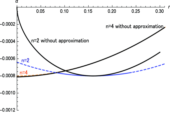
Figure 1: The relation between $r$ and $\alpha$ for $n_{s}=0.96$. The dashed blue curve is Eq. (27) derived assuming $|\xi|\ll 1$, while the upper left black one is the curve derived without assuming $|\xi|\ll 1$. The dashed orange curve is Eq. (32) derived assuming $|\xi|\ll 1$, which almost overlaps with the black one derived without assuming $|\xi|\ll 1$.

III.1.3 $n(\neq 4)$

For general $n(\neq 4)$, from Eqs. (11)-(13), we obtain

$$\alpha=\frac{(n+2)\left(3n^{3}-32n^{2}+88n-64\right)}{64(n-12)^{2}n^{2}}r^{2}+\frac{(n+2)\left(5n^{2}-48n+80\right)}{8(n-12)^{2}n}r(n_{s}-1)$$

$$\qquad+\frac{2(n+2)(n-8)}{(n-12)^{2}}(n_{s}-1)^{2},$$ (34)

$$(12-n)\left(\left(8(n-1)-n^{2}\right)r-8n(8-n)(1-n_{s})\right)<0\,.$$ (35)

III.2 $n=4$ with $|\xi|\gg 1$

For $n=4$ with $|\xi|\gg 1$, Eqs. (17)-(19) become

$$r = \frac{64}{3\xi^{2}\phi^{4}},$$ (36)

$$n_{s}-1 = \frac{8}{3\xi\phi^{2}},$$ (37)

$$\alpha = -\frac{32}{9\xi^{2}\phi^{4}}\,.$$ (38)

Hence we obtain

$$\alpha=-\frac{1}{2}(n_{s}-1)^{2}=-\frac{1}{6}r\,,$$ (39)

which may be called ”Starobinsky attractor” according to klr .

In Fig. 2, we show the relations Eq. (27), Eq. (32), and Eq. (39) in the $(r,\alpha)$ plane for $n_{s}=0.96$. Black points are for $\xi=0$, the left (right) of which corresponds to $\xi<0(\xi>0)$. Solid curves are for $|\xi|<10^{-3}$. Orange point is for $|\xi|\gg 1$ (Eq. (39)). Fig. 3 shows the regions scanned by the relations Eq. (32) and Eq. (39) for $0.955<n_{s}<0.965$. We find that $\alpha$ is insensitive to $\xi$. For $\xi<0$, $\alpha$ is constrained in the narrow range: $-8\times 10^{-4}<\alpha<-6\times 10^{-4}$ for $n_{s}=0.96$, and $-10^{-3}<\alpha<-4\times 10^{-4}$ for $0.955<n_{s}<0.965$.

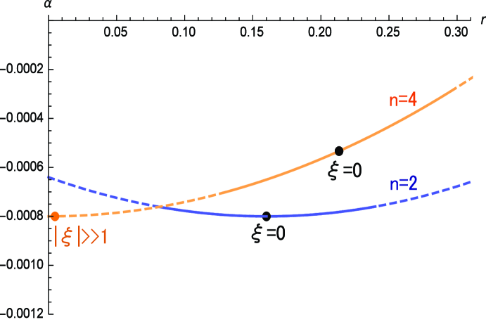
Figure 2: Consistency relations for the nonminimally coupled chaotic inflation model with $n=2$ (dashed blue) and $n=4$ (dashed orange) for $n_{s}=0.96$ in $(r,\alpha)$ plane. Black points are for $\xi=0$. Solid curves are for $|\xi|<10^{-3}$. Orange point is for $|\xi|\gg 1$ (Eq. (39)). Note that the dashed blue curve is inaccurate.

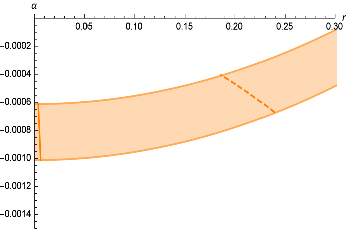
Figure 3: Consistency relations for the nonminimally coupled chaotic inflation model with a quartic potential for $0.955<n_{s}<0.965$ in $(r,\alpha)$ plane. Dashed curves are for $\xi=0$. Solid orange curve is for $|\xi|\gg 1$ (Eq. (39)).

III.3 General $n$ for fixed $\xi$.

Lastly, we provide a consistency relation for general $n$ for fixed $\xi$ with $|\xi|\ll 1$. From Eqs. (11)-(12), $n$ and $\phi^{2}$ are written in terms of $r$, $n_{s}$, and $\xi$ :

$$n = \frac{192\xi-r-8(n_{s}-1)-\sqrt{(r+8(n_{s}-1-24\xi))^{2}-128\xi r}}{32\xi},$$ (40)

$$\phi^{2} = \frac{r+8(n_{s}-1)-192\xi+\sqrt{(r+8(n_{s}-1-24\xi))^{2}-128\xi r}}{2\xi(r+8(n_{s}-1-8\xi))}.$$ (41)

Then, from Eq. (13), $\alpha$ can be written as a function of $r$ and $n_{s}$, which is too complicated to show here.

In Fig. 4, we plot $\alpha$ as a function of $r$ for $n_{s}=0.96$. $\xi=-10^{-3},0,10^{-3}$ from top to bottom. The curves for $n=2$ and $n=4$ are also shown. We find that the consistency relation for $\xi=0$ ($\alpha=-(1-n_{s})^{2}+\frac{1}{8}r(1-n_{s})$ ) derived in ck does not change so much as long as $|\xi|<10^{-3}$. For general $n$, varying $\xi$ changes $\alpha$ by $O(10^{-3})$. If $r<0.1$, then $\alpha$ is constrained in the range of $-2.7\times 10^{-3}<\alpha<-8\times 10^{-4}$.

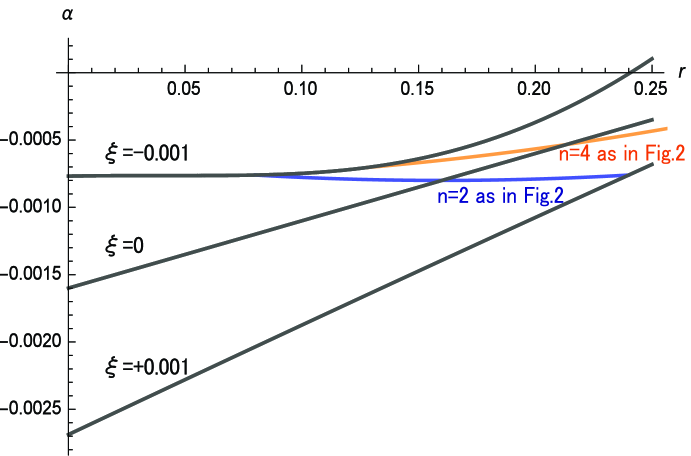
Figure 4: Consistency relations for the nonminimally coupled chaotic inflation model with $\xi=-10^{-3},0,10^{-3}$ from top to bottom for $n_{s}=0.96$. Blue (orange) curve corresponds to $n=2(n=4)$ as in Fig. 2.

IV Summary

We have derived consistency relations for chaotic inflation with a nonminimal coupling $\xi$. For a quadratic potential, we find that although the tensor-to-scalar ratio $r$ is sensitive to $\xi$, the running of the spectral index $\alpha$ is rather insensitive to the change in $\xi$ as long as $\xi$ is small. For a quartic potential, we find that $\alpha$ is insensitive to $\xi$ even for large $|\xi|$. We also find that the consistency relation for a general monomial potential does not change so much by changing $\xi$ as long as $|\xi|\leq 10^{-3}$.

If $r<0.1$, then $\xi<0$ and $\alpha\simeq-8\times 10^{-4}$ are implied for a quartic potential. Even for a general monomial potential, $r<0.1$ forces $\alpha$ to be in the range $-2.7\times 10^{-3}<\alpha<-8\times 10^{-4}$ for $n_{s}=0.96$ as long as $|\xi|<10^{-3}$ . Since $\alpha$ is found to be insensitive to $\xi$, this $\alpha$ may be regarded as the prediction for the chaotic potential irrespective of the nonminimal coupling. Measurement of $\alpha$ with a precision of $O(10^{-3})$ by future observations of the 21 cm line kohri will be crucially important in pinning down the inflation model.

Note added in proof: A recent joint analysis of BICEP2/Keck Array and Planck data yields an upper limit $r<0.12$ bicep2planck .

References

(1)
P. A. R. Ade et al. [BICEP2 Collaboration],
Phys. Rev. Lett. 112, 241101 (2014)
[arXiv:1403.3985 [astro-ph.CO]].
(2)
T. Chiba and K. Kohri,
PTEP 2014, no. 9, 093E01 (2014)
[arXiv:1406.6117 [astro-ph.CO]].
(3)
T. Futamase and K. i. Maeda,
Phys. Rev. D 39, 399 (1989).
(4)
D. S. Salopek, J. R. Bond and J. M. Bardeen,
Phys. Rev. D 40, 1753 (1989);
F. L. Bezrukov and M. Shaposhnikov,
Phys. Lett. B 659, 703 (2008)
[arXiv:0710.3755 [hep-th]].
(5)
A. A. Starobinsky,
Phys. Lett. B 91, 99 (1980).
(6)
N. Makino and M. Sasaki,
Prog. Theor. Phys. 86, 103 (1991).
(7)
T. Chiba and M. Yamaguchi,
JCAP 0810, 021 (2008)
[arXiv:0807.4965 [astro-ph]].
(8)
R. Catena, M. Pietroni and L. Scarabello,
Phys. Rev. D 76, 084039 (2007)
[astro-ph/0604492].
(9)
T. Chiba and M. Yamaguchi,
JCAP 1310, 040 (2013)
[arXiv:1308.1142 [gr-qc]].
(10)
S. Tsujikawa, J. Ohashi, S. Kuroyanagi and A. De Felice,
Phys. Rev. D 88, 023529 (2013).
(11)
P. A. R. Ade et al. [Planck Collaboration],
arXiv:1303.5082 [astro-ph.CO].
(12)
Y. Hamada, H. Kawai, K. y. Oda and S. C. Park,
arXiv:1408.4864 [hep-ph].
(13)
R. Kallosh, A. Linde and D. Roest,
Phys. Rev. Lett. 112, 011303 (2014)
[arXiv:1310.3950 [hep-th]];
R. Kallosh, A. Linde and D. Roest,
arXiv:1407.4471 [hep-th];
B. Mosk and J. P. van der Schaar,
arXiv:1407.4686 [hep-th].
(14)
S. Dodelson and L. Hui,
Phys. Rev. Lett. 91, 131301 (2003)
[astro-ph/0305113].
(15)
A. R. Liddle and S. M. Leach,
Phys. Rev. D 68, 103503 (2003)
[astro-ph/0305263].
(16)
K. Kohri, Y. Oyama, T. Sekiguchi and T. Takahashi,
JCAP 1310, 065 (2013).
(17)
P. A. R. Ade et al. [BICEP2/Keck Array and Planck collaborations],
arXiv:1502.00612 [astro-ph.CO].