Robust quantum state transfer using tunable couplers

Abstract

We analyze the transfer of a quantum state between two resonators connected by a superconducting transmission line. Nearly perfect state-transfer efficiency can be achieved by using adjustable couplers and destructive interference to cancel the back-reflection into the transmission line at the receiving coupler. We show that the transfer protocol is robust to parameter variations affecting the transmission amplitudes of the couplers. We also show that the effects of Gaussian filtering, pulse-shape noise, and multiple reflections on the transfer efficiency are insignificant. However, the transfer protocol is very sensitive to frequency mismatch between the two resonators. Moreover, the tunable coupler we considered produces time-varying frequency detuning caused by the changing coupling. This detuning requires an active frequency compensation with an accuracy better than $90\%$ to yield the transfer efficiency above $99\%$.

I Introduction

The realization of quantum networks composed of many nodes requires high-fidelity protocols that transfer quantum states from site to site by using “flying qubits” Kim08 ; DiVincenzo-00 . The standard idea of the state transfer between two nodes of a quantum network Cir97 assumes that the state of a qubit is first encoded onto a photonic state at the emitting end, after which the photon leaks out and propagates through a transmission line to the receiving end, where its state is transferred onto the second qubit. The importance of quantum state transfer has stimulated significant research activity in optical realizations of such protocols, e.g., Braunstein-98 ; Furusawa-98 ; Lloyd-01 , including trapping of photon states in atomic ensembles Duan-01 ; Lukin-03 ; Chou-05 ; Razavi-06 . Recent experimental demonstrations include the transfer of an atomic state between two distant nodes Rem12 and the transfer between an ion and a photon Bla13 .

An important idea for state transfer in the microwave domain is to use tunable couplers between the quantum oscillators and the transmission line Jah07 ; Kor11 (the idea is in general similar to the idea proposed in Ref. Cir97 for an optical system). In particular, this strategy is natural for superconducting qubits, for which a variety of tunable couplers have been demonstrated experimentally Hime-06 ; Niskanen-07 ; Allman-10 ; Bialczak-11 ; Hoffman-11 ; Yin13 ; Sri14 ; Wen14 ; Chen-14 ; Whittaker-14 ; Pierre-14 (these couplers are important for many applications, e.g., Clarke-08 ; Gambetta-11 ; Sete-13 ; You-14 ). Although there has been rapid progress in superconducting qubit technology, e.g. Barends-14 ; Chow-14 ; Weber-14 ; Sun-14 ; NEC-14 ; Stern-14 ; Wal13 ; Gustavsson-13 ; Riste-13 , most of the experiments so far are limited to a single chip or a single resonator in a dilution refrigerator (an exception is Roch-14 ). Implementing the quantum state transfer between remote superconducting qubits, resonators, or even different refrigerators using “flying” microwave qubits propagating through lossless superconducting waveguides would significantly extend the capability of the technology (eventually permitting distributed quantum computing and quantum communications over extended distances using quantum repeaters). The essential ingredients of the transfer protocol proposed in Ref. Kor11 have already been demonstrated experimentally. The emission of a proper (exponentially increasing) waveform of a quantum signal has been demonstrated in Ref. Sri14 , while the capture of such a waveform with 99.4% efficiency has been demonstrated in Ref. Wen14 . The combination of these two procedures in one experiment would demonstrate a complete quantum state transfer (more precisely, the complete first half of the procedure of Ref. Kor11 ). Note that Refs. Sri14 and Wen14 used different tunable couplers: a “tunable mirror” Yin13 between the resonator and the transmission line in Ref.  Wen14 and a tunable coupling between the qubit and the resonator Hoffman-11 (which then rapidly decays into the transmission line) in Ref. Sri14 . However, this difference is insignificant for the transfer protocol of Ref. Kor11 . Another promising way to produce shaped photons is to use a modulated microwave drive to couple the superconducting qubit with the resonator Pechal2014 ; Zeytinoglu2015 (see also Refs. Keller2004 ; Kolchin2008 for implementation of optical techniques for shaped photons).

In this work we extend the theoretical analysis of the state transfer protocol proposed in Ref. Kor11 , focusing on its robustness against various imperfections. In our protocol a quantum state is transferred from the emitting resonator to the receiving resonator through a transmission line (the state transfer using tunable coupling directly between the qubit and the transmission line has also been considered in Ref. Kor11 , but we do not discuss it here). The procedure essentially relies on the cancellation of back-reflection into the transmission line via destructive interference at the receiving end, which is achieved by modulation of the tunable couplers between the resonators and the transmission line. (Note that the protocol is often discussed in terms of a “time reversal”, following the terminology of Ref. Cir97 ; however, we think that discussion in terms of a destructive interference is more appropriate.) In Ref. Kor11 , it was shown that nearly perfect transfer efficiency can be achieved if identical resonators and proper time-varying transmission amplitudes of the two couplers are used. However, in obtaining this high-efficiency state transfer, only ideal design parameters were assumed. Also, various experimentally relevant effects, including multiple reflections and frequency mismatch between the two resonators, were not analyzed quantitatively.

In this paper we study in detail (mostly numerically) the effect of various imperfections that affect the transmission amplitudes of the couplers. In the simulations we focus on two values for the design efficiency: 0.99 and 0.999. The value of 0.99 crudely corresponds to the current state of the art for the two-qubit quantum gate fidelities Barends-14 and threshold of some quantum codes Fowler2012 ; we believe that the state transfer with 0.99 efficiency may already be interesting for practical purposes, while the value of 0.999 would be the next natural milestone for the experimental quantum state transfer. We find that the transfer protocol is surprisingly robust to parameter variations, with a typical decrease in the efficiency of less than 1% for a 5% variation of the design parameters (the scaling is typically quadratic, so half of the variation produces a quarter of the effect). We also study the effect of Gaussian filtering of the signals and find that it is practically negligible. The addition of noise to the ideal waveforms produces only a minor decrease in the transfer efficiency. Numerical analysis of multiple reflections also shows that the corresponding effect is not significant and can increase the inefficiency by at most a factor of two. The analysis of the effect of dissipative losses is quite simple and, as expected, shows that a high-efficiency state transfer requires a low-loss transmission line and resonators with energy relaxation times much longer than duration of the procedure.

A major concern, however, is the effect of frequency mismatch between the two resonators, since the destructive interference is very sensitive to the frequency detuning. We consider two models: a constant-in-time detuning and a time-dependent detuning due to changing coupling. For the latter model we use the theory of the coupler realized in Refs. Yin13 ; Wen14 ; the frequency variation due to the coupling modulation has been observed experimentally Yin13 . Our results show that a high-efficiency state transfer is impossible without an active compensation of the frequency change; the accuracy of this compensation should be at least within the 90%-95% range.

Although we assume that the state transfer is performed between two superconducting resonators, using the tunable couplers of Refs. Yin13 ; Wen14 , our analysis can also be applied to other setups, for example, schemes based on tunable couplers between the qubits and the transmission line or based on the tunable couplers between the qubits and the resonators Hoffman-11 ; Sri14 ; Pechal2014 ; Zeytinoglu2015 , which are then strongly coupled with the transmission line. Note that the frequency change compensation is done routinely in the coupler of Refs. Hoffman-11 ; Sri14 , thus giving a natural way to solve the problem of frequency mismatch. Similarly, the phase is naturally tunable in the coupler of Refs. Pechal2014 ; Zeytinoglu2015 .

The paper is organized in the following way. In Sec. II we discuss the ideal state transfer protocol, its mathematical model, and the relation between classical transfer efficiency (which is mostly used in this paper) and quantum state/process fidelity. In Sec. III we analyze the decrease of the transfer efficiency due to deviations from the design values of various parameters that define the transmission amplitudes of the couplers. We also study the effects of pulse-shape warping, Gaussian filtering, noise, and dissipative losses. In Sec. IV we analyze the effect of multiple reflections of the back-reflected field on the transfer efficiency. The effect of frequency mismatch between the two resonators is discussed in Sec. V. Finally, we summarize the main results of the paper in Sec. VI. Appendix A is devoted to the quantum theory of a beam splitter, which is used to relate the efficiency of a classical state transfer to the fidelity of a quantum state transfer. In Appendix B we discuss the theory of the tunable coupler of Refs. Yin13 ; Wen14 and find the frequency detuning caused by the coupling variation.

II Model and transfer protocol

II.1 Model

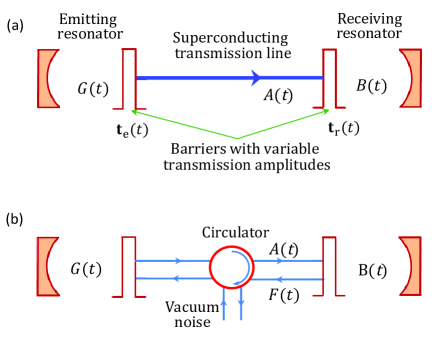
Figure 1: (a) The state transfer setup. An initial microwave field amplitude $G(0)$ is transferred from the emitting resonator to the receiving resonator via a transmission line. This is done using variable couplers for both resonators, characterized by (effective) transmission amplitudes ${\bf t}_{\rm e}(t)$ and ${\bf t}_{\rm r}(t)$, and corresponding leakage rates $\kappa_{\rm e}(t)$ and $\kappa_{\rm r}(t)$. Almost perfect transfer can be achieved when the back-reflection of the propagating field $A(t)$ is cancelled by arranging its destructive interference with the leaking part of the field $B(t)$ in the receiving resonator. (b) A variant of the setup that includes a circulator, which prevents multiple reflections of the small back-reflected field $F(t)$.

We consider the system illustrated in Fig. 1(a). A quantum state is being transferred from the emitting (left) resonator into the initially empty receiving (right) resonator via the transmission line. This is done by using time-varying couplings (“tunable mirrors”) between the resonators and the transmission line. The (effective) transmission amplitudes ${\bf t}_{\rm e}$ and ${\bf t}_{\rm r}$ for the emitting and receiving resonator couplers, respectively, as a function of time $t$ are illustrated in Fig. 2. As discussed later, the main idea is to almost cancel the back-reflection into the transmission line from the receiving resonator by using destructive interference. Then the field leaking from the emitting resonator is almost fully absorbed into the receiving resonator. Ideally, we want the two resonators to have equal frequencies, $\omega_{\rm e}=\omega_{\rm r}$; however, in the formalism we will also consider slightly unequal resonator frequencies $\omega_{\rm e}(t)$ and $\omega_{\rm r}(t)$. We assume large quality factors $Q$ for both resonators by assuming $|{\bf t}_{\rm e}(t)|\ll 1$ and $|{\bf t}_{\rm r}(t)|\ll 1$ (the maximum value is crudely $|{\bf t}_{\rm e(r),max}|\sim 0.05$, leading to $Q_{\rm min}\sim 10^{3}$ – see later), so that we can use the single-mode approximation. For simplicity, we assume a dispersionless transmission line.

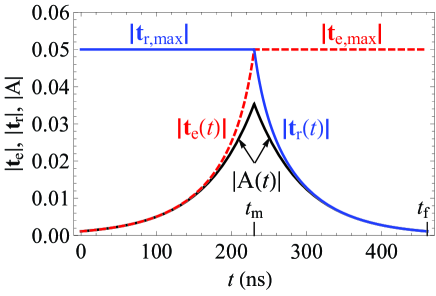
Figure 2: Time dependence (“pulse shapes”) of the absolute values of transmission amplitudes ${\bf t}_{\rm e}(t)$ for the emitting coupler (red dashed curve) and ${\bf t}_{\rm r}(t)$ for the receiving coupler (blue solid curve). The amplitude ${\bf t}_{\rm e}(t)$ is kept constant at the maximum level $\textbf{t}_{\rm e,max}$ after the mid-time $t_{\rm m}$, while ${\bf t}_{\rm r}(t)$ is kept at the maximum $\textbf{t}_{\rm r,max}$ during the first part of the procedure, $t\leq t_{\rm m}$. The propagating field $A(t)$ first increases exponentially and then decreases exponentially (black solid curve). In simulations we typically use $|\textbf{t}_{\rm e,max}|=|\textbf{t}_{\rm r,max}|=0.05$ for quarter-wavelength 6 GHz resonators ($\tau_{\rm e}=\tau_{\rm r}=33$ ns); then the transfer efficiency $\eta=0.999$ requires the procedure duration of $t_{\rm f}=460$ ns.

We will mostly analyze a classical field transfer between the two resonators, with a straightforward relation to the quantum case, discussed later. The notations $G(t)$ and $B(t)$ correspond to the field amplitudes in the emitting and receiving resonators [see Fig. 1(a)], while $A(t)$ describes the propagating field in the transmission line. However, in contrast to the notations of Ref. Kor11 , here we use dimensionless $G$ and $B$, normalizing the field amplitudes Walls-book ; Ger06 in such a way that for classical (coherent) fields, $|G|^{2}$ and $|B|^{2}$ are equal to the average number of photons in the resonators. Similarly, the normalization of $A$ is chosen so that $|A|^{2}$ is the number of propagating photons per second. Such normalizations for resonators are more appropriate for the analysis of quantum information. Also, with this normalization, the amplitudes will not change with adiabatically-changing resonator frequency, in contrast to the usual field amplitudes.

In most of the analysis we assume (unless mentioned otherwise) that the transmission line is either long or contains a circulator [Fig. 1(b)], so that we can neglect the multiple reflections of the small back-propagating field $F(t)$ (the effect of multiple reflections will be considered in Sec. IV). We also assume that there is no classical noise entering the emitting resonator from the circulator (only vacuum noise).

With these assumptions and normalizations, the time dynamics of the classical field amplitudes is described in the rotating frame by the equations

$$\dot{G}=-i\Delta\omega_{\rm e}G-\frac{1}{2}\left(\kappa_{\rm e}+T_{1,\rm e}^{-1}\right)G,$$ (1)

$$\dot{B}=-i\Delta\omega_{\rm r}B-\frac{1}{2}\left(\kappa_{\rm r}+T_{1,\rm r}^{-1}\right)B+\frac{\textbf{t}_{\rm r}}{|\textbf{t}_{\rm r}|}\sqrt{\kappa_{\rm r}}\,A,$$ (2)

$$A=\sqrt{\eta_{\rm tl}}\,\frac{\textbf{t}_{\rm e}}{|\textbf{t}_{\rm e}|}\sqrt{\kappa_{\rm e}}\,G,$$ (3)

where $\Delta\omega_{\rm e}=\omega_{\rm e}-\omega_{0}$ and $\Delta\omega_{\rm r}=\omega_{\rm r}-\omega_{0}$ are small detunings (possibly changing slowly with time) from the (arbitrary) rotating frame frequency $\omega_{0}(t)$, the decay rates $\kappa_{\rm e}$ and $\kappa_{\rm r}$ are due to leakage into the transmission line, while additional losses are described by the energy relaxation times $T_{1,\rm e}$ and $T_{1,\rm r}$ in the resonators and imperfect transfer efficiency $\eta_{\rm tl}$ of the transmission line. Note that $A$ has the dimension of $1/\sqrt{\rm s}$ in contrast to the dimensionless $G$ and $B$, so that the factors $\sqrt{\kappa_{\rm e(r)}}$ restore the proper dimension. The leakage rates are

$$\kappa_{\rm e}(t)=\frac{|\tilde{\bf{t}}^{\rm in}_{\rm e}|^{2}}{\tau_{\rm rt,e}}\frac{R_{\rm e}}{R_{\rm tl}}=\frac{|\textbf{t}_{\rm e}|^{2}}{\tau_{\rm rt,e}},\,\,\,\kappa_{\rm r}(t)=\frac{|\tilde{\bf{t}}^{\rm in}_{\rm r}|^{2}}{\tau_{\rm rt,r}}\frac{R_{\rm r}}{R_{\rm tl}}=\frac{|\textbf{t}_{\rm r}|^{2}}{\tau_{\rm rt,r}},$$ (4)

where $\tilde{\bf{t}}_{\rm e}^{\rm in}$ and $\tilde{\bf{t}}_{\rm r}^{\rm in}$ are the transmission amplitudes of the couplers (for a wave incident from inside of the resonators), $\tau_{\rm rt,e}$ and $\tau_{\rm rt,r}$ are the round-trip times in the resonators, $R_{\rm e}$, $R_{\rm r}$, and $R_{\rm tl}$ are the wave impedances of the resonators and the transmission line, while $\textbf{t}_{\rm e}=\tilde{\bf{t}}_{\rm e}^{\rm in}\sqrt{R_{\rm e}/R_{\rm tl}}$ and $\textbf{t}_{\rm r}=\tilde{\bf{t}}_{\rm r}^{\rm in}\sqrt{R_{\rm r}/R_{\rm tl}}$ are the effective transmission amplitudes. Note that the transmission amplitudes $\tilde{\bf t}$ depend on the wave direction (from inside or outside of a resonator), while the effective transmission amplitudes $\bf t$ do not. For convenience we will be working with the effective transmission amplitudes $\textbf{t}_{\rm e}$ and $\textbf{t}_{\rm r}$, so that we do not need to worry about possibly unequal wave impedances. For quarter-wavelength resonators $\tau_{\rm rt,e}\approx\pi/\omega_{\rm e}\approx\pi/\omega_{0}$ and $\tau_{\rm rt,r}\approx\pi/\omega_{\rm r}\approx\pi/\omega_{0}$, so the quality factors are

$$Q_{\rm e(r)}=\frac{\omega_{\rm e(r)}}{\kappa_{\rm e(r)}}\approx\frac{\pi}{|\textbf{t}_{\rm e(r)}|^{2}}.$$ (5)

Note that the phase factors $\textbf{t}_{\rm r}/|\textbf{t}_{\rm r}|$ and $\textbf{t}_{\rm e}/|\textbf{t}_{\rm e}|$ in Eqs. (2) and (3) may change in time because of changing coupling Kor11 ; Yin13 (as discussed later in Sec. V B and Appendix B); this is why these somewhat unusual factors cannot be neglected. Strictly speaking, the last term in Eq. (2) should also be multiplied by $\sqrt{\omega_{\rm e}/\omega_{\rm r}}$; this is because of different normalizations, related to different photon energies $\hbar\omega_{\rm e}$ and $\hbar\omega_{\rm r}$ in the resonators. However, we neglect this correction, assuming a relatively small detuning. Note that the effective propagation time along the transmission line is zero in Eqs. (1)–(3) since we use appropriately shifted clocks (here the assumption of a dispersionless transmission line is necessary); however, the physical propagation time will be important in the analysis of multiple reflections in Sec. IV. Also note that to keep Eqs. (1)–(3) reasonably simple, we defined the phases of $B$ and $G$ to be somewhat different from the actual phases of the standing waves in the resonators (see discussion in Sec. II C).

Even though in Eqs. (1)–(3) we use normalized fields $G$, $B$, and $A$, which imply discussion in terms of the photon number, below we will often use the energy terminology and invoke the arguments of the energy conservation instead of the photon number conservation. At least in the case without detuning the two pictures are fully equivalent, but the energy language is more intuitive, and thus preferable. This is why in the following we will use the energy and photon number terminology interchangeably.

II.2 Efficiency and fidelity

We will characterize performance of the protocol via the transfer efficiency $\eta$, which is defined as the ratio between the energy of the field (converted into the photon number) in the receiving resonator at the end of the procedure, $t=t_{\rm f}$, and the energy (photon number) at the initial time, $t=0$, in the emitting resonator:

$$\eta=\frac{|B(t_{\rm f})|^{2}}{|G(0)|^{2}}.$$ (6)

We emphasize that in this definition we assume that only the emitting resonator has initially a non-zero field.

As we discuss in this section, the classical efficiency $\eta$ is sufficient to characterize the quantum transfer as well, so that the quantum state and process fidelities derived below are directly related to $\eta$ (this requires assumption of vacuum everywhere except the initial state of the emitting resonator). The idea of the conversion between the classical and quantum transfers is based on the linearity of the process, and thus can be analyzed in essentially the same way as the quantum optical theory of beam splitters, discussed in Appendix A.

Let us focus on the case with the circulator [Fig. 1(b)] in the absence of dissipative losses ($T_{1,\rm e}^{-1}=T_{1,\rm r}^{-1}=0$, $\eta_{\rm tl}=1$). In general, there is a linear input-output relation between the fields at $t=0$ and the fields at $t=t_{\rm f}$. This relation is the same for the classical fields and the corresponding quantum operators in the Heisenberg picture (Yurke-84 ; Jah07 ), so for simplicity we discuss the classical fields. The relevant fields at $t=0$ are $G(0)$, $B(0)$, and the (infinite number of) temporal modes propagating towards the emitting resonator through the circulator; these modes can be described as time-dependent field $V(t)$, where $t$ corresponds to the time, at which the field arrives to the emitting resonator. Note that $B(0)$ and $V(t)$ are assumed to be zero in our protocol; however, we need to take them into account explicitly, because in the quantum language they would correspond to operators, representing vacuum noise (with the standard commutation relations). The fields at the final time $t=t_{\rm f}$ are $B(t_{\rm f})$, $G(t_{\rm f})$, and the collection of the outgoing back-reflected fields $F(t)$ for $0\leq t\leq t_{\rm f}$ [see Fig. 1(b)]. Note that normalization of the propagating fields $V(t)$ and $F(t)$ is similar to the normalization of $A(t)$.

The input-output relation $\{G(0),B(0),V(t)|_{0\leq t\leq t_{\rm f}}\}\mapsto\{G(t_{\rm f}),B(t_{\rm f}),F(t)|_{0\leq t\leq t_{\rm f}}\}$ is linear and unitary, physically because of the conservation of the number of photons (energy). In particular,

$$B(t_{\rm f})=\sqrt{\eta}\,e^{i\varphi_{\rm f}}G(0)+w_{B}B(0)+\int_{0}^{t_{\rm f}}w_{V}(t)V(t)\,dt,$$ (7)

where $\eta$ is obviously given by Eq. (6), $\varphi_{\rm f}$ is the phase shift between $B(t_{\rm f})$ and $G(0)$, while $w_{B}$ and $w_{V}(t)$ are some weight factors in this general linear relation. These weight factors can be calculated by augmenting Eqs. (1)–(3) to include $V(t)$ and $F(t)$, but we do not really need them to find the quantum transfer fidelity if $B(0)$ and $V(t)$ correspond to vacuum. Note that the unitarity of the input-output transformation requires the relation

$$\eta+|w_{B}|^{2}+\int_{0}^{t_{\rm f}}|w_{V}(t)|^{2}\,dt=1$$ (8)

(sum of squared absolute values of elements in a row of a unitary matrix equals one), where we neglected the slight change in the normalization (discussed above) in the case of time-varying detuning.

This picture of the input-output relations can in principle be extended to include non-zero $T_{1,\rm e(r)}^{-1}$ and/or $\eta_{\rm tl}\neq 1$; for that we would need to introduce additional noise sources, which create additional terms in Eqs. (7) and (8) similar to the terms from the noise $V$. Also, if we consider the case without the circulator, the structure of these equations remains similar, but the role of $V(t)$ is played by the temporal modes of the initial field propagating in the transmission line from the receiving to the emitting resonator (since clocks are shifted along the transmission line, there is formally no field “stored” in the transmission line, which propagates from the emitting to the receiving resonator).

Using the framework of the linear input-output relation, Eq. (7) derived for classical fields can also be used to describe the quantum case. This can be done using the standard quantum theory of beam splitters Ger06 (see Appendix A), by viewing Eq. (7) as the result of mixing the fields $G(0)$, $B(0)$, and an infinite number of fields (temporal modes) $V(t)$ with beam splitters to produce the proper linear combination. Importantly, if $B(0)$ corresponds to vacuum and $V(t)$ also corresponds to vacuum, then we can assume only one beam splitter with the proper transfer amplitude $\sqrt{\eta}\,e^{i\varphi_{\rm f}}$ for $G(0)\rightarrow B(t_{\rm f})$; this is because a linear combination of several vacua is still the vacuum. Equivalently, the resulting quantum state in the receiving resonator is equal to the initial quantum state of the emitting resonator, subjected to the phase shift $\varphi_{\rm f}$ and leakage (into vacuum) described by the (classical) efficiency $\eta$. The same remains correct in the presence of nonzero relaxation rates $T_{1,\rm e}^{-1}$ and $T_{1,\rm r}^{-1}$ and imperfect $\eta_{\rm tl}$ if these processes occur at zero effective temperature (involving only vacuum noise).

As shown in Appendix A, if the initial state in the emitting resonator is $|\psi_{\rm in}\rangle=\sum_{n}\alpha_{n}|n\rangle$ in the Fock space ($\sum_{n}|\alpha_{n}|^{2}=1$), then the final state of the receiving resonator is represented by the density matrix, which can be obtained from the state $|\psi_{\rm fin}\rangle=\sum_{n,k}\alpha_{n+k}\sqrt{(n+k)!/n!k!}\,\eta^{n/2}(1-\eta)^{k/2}e^{i(n+k)\varphi_{\rm f}}|n\rangle|k\rangle_{\rm a}$ by tracing over the ancillary state $|k\rangle_{\rm a}$ (this ancilla corresponds to the second outgoing arm of the beam splitter). This gives the density matrix $\rho_{\rm fin}=\sum_{j,n,m}\alpha_{n+j}\alpha^{*}_{m+j}\sqrt{(n+j)!(m+j)!}(j!\sqrt{n!m!})^{-1}\eta^{(n+m)/2}\\ (1-\eta)^{j}e^{i(n-m)\varphi_{\rm f}})|n\rangle\langle m|$. The state fidelity (overlap with the initial state) is then

$$F_{\rm st} =\sum_{j,n,m}\frac{\sqrt{(n+j)!(m+j)!}}{j!\sqrt{n!m!}}\,\alpha_{n}^{*}\alpha_{m}\alpha_{n+j}\alpha^{*}_{m+j}$$

$$\hskip 14.22636pt\times\eta^{(n+m)/2}(1-\eta)^{j}e^{i(n-m)\varphi_{\rm f}}.$$ (9)

Note that the phase shift $\varphi_{\rm f}$ can easily be corrected in an experiment (this correction is needed anyway for resonators, which are significantly separated in space), and then the factor $e^{i(n-m)\varphi_{\rm f}}$ in Eq. (9) can be removed.

The discussed quantum theory (at zero temperature, i.e., with only vacuum noise) becomes very simple if we transfer a qubit state $|\psi_{\rm in}\rangle=\alpha|0\rangle+\beta|1\rangle$. Then the resulting state is

$$|\psi_{\rm fin}\rangle=\alpha|0\rangle|0\rangle_{\rm a}+\beta e^{i\varphi_{\rm f}}(\sqrt{\eta}\,|1\rangle|0\rangle_{\rm a}+\sqrt{1-\eta}\,|0\rangle|1\rangle_{\rm a}),$$ (10)

where the ancillary states $|1\rangle_{\rm a}$ and $|0\rangle_{\rm a}$ indicate whether a photon was lost to the environment or not. After tracing $|\psi_{\rm fin}\rangle\langle\psi_{\rm fin}|$ over the ancilla we obtain density matrix

$$\rho_{\rm fin}=\left(\begin{array}[]{cc}\eta|\beta|^{2}&\sqrt{\eta}\,e^{i\varphi_{\rm f}}\alpha^{*}\beta\\ \sqrt{\eta}\,e^{-i\varphi_{\rm f}}\alpha\beta^{*}&|\alpha|^{2}+|\beta|^{2}(1-\eta)\end{array}\right).$$ (11)

Note that since a qubit state contains at most one excitation, the essential dynamics occurs only in the single-photon subspace. Therefore, it is fully equivalent to the dynamics of classical fields (with field amplitudes replaced by probability amplitudes). Thus, Eq. (10) can be written directly, without using the quantum beam splitter approach, which is necessary only for multi-photon states.

In quantum computing the qubit state transfer (quantum channel) is usually characterized by the quantum process fidelity $F_{\chi}$ or by the average state fidelity $\overline{F}_{\rm st}$, which are related as Nie02 ; Hor99 $1-F_{\chi}=(1-\overline{F}_{\rm st})\times 3/2$. In order to calculate $F_{\chi}$, we calculate state fidelity $F_{\rm st}$ (overlap with initial state) and then average it over the Bloch sphere. Neglecting the phase $\varphi_{\rm f}$, which can be easily corrected in an experiment, from Eq. (11) we find $F_{\rm st}=|\alpha|^{4}+\eta|\beta|^{4}+|\alpha\beta|^{2}(1-\eta+2\sqrt{\eta})$, which also follows from Eq. (9). To average this fidelity over the Bloch sphere of initial states, it is sufficient Nie02 (see also Kea12 ) to average it over only six states: $|0\rangle$, $|1\rangle$, $(|0\rangle\pm|1\rangle)/\sqrt{2}$, and $(|0\rangle\pm i|1\rangle)/\sqrt{2}$. This gives $\overline{F}_{\rm st}=(3+\eta+2\sqrt{\eta})/6$, which can be converted into the process fidelity

$$F_{\chi}=\frac{1}{4}(1+\sqrt{\eta})^{2}.$$ (12)

This equation gives the relation between the classical energy transfer efficiency $\eta$ which we use in this paper and the process fidelity $F_{\chi}$ used in quantum computing. Note the relation $1-F_{\chi}\approx(1-\eta)/2$ when $\eta\approx 1$. Also note that a non-vacuum noise contribution (due to finite temperature) always decreases $F_{\chi}$ (see Appendix A). If the phase shift $\varphi_{\rm f}$ is included in the definition of fidelity (assuming that $\varphi_{\rm f}$ is not corrected), then Eq. (12) becomes $F_{\chi}=(1+\eta+2\sqrt{\eta}\cos\varphi_{\rm f})/4$.

Thus, in this section we have shown that the state and the process fidelities of the quantum state transfer are determined by the classical efficiency $\eta$ and experimentally correctable phase shift $\varphi_{\rm f}$. This is why in the rest of the paper we analyze the efficiency $\eta$ of essentially a classical state transfer.

II.3 Transfer procedure

Now let us describe the transfer protocol, following Ref. Kor11 (this will be the second protocol out of two slightly different procedures considered in Ref. Kor11 ). Recall that we consider normalized classical field amplitudes. The main idea of achieving nearly perfect transfer is to use time-dependent transmission amplitudes $\textbf{t}_{\rm e}$ and $\textbf{t}_{\rm r}$ to arrange destructive interference between the field $A$ reflected from the receiving resonator and the part of field $B$ leaking through the coupler (see Fig. 1). Thus, we want the total back-reflected field $F(t)$ to nearly vanish: $F(t)\approx 0$, where

$$F=\frac{\textbf{r}_{\rm r}^{\rm out}}{|\textbf{r}_{\rm r}|}\,A+\frac{\textbf{t}_{\rm r}}{|\textbf{t}_{\rm r}|}\,\sqrt{\kappa_{\rm r}}\,\frac{|\textbf{r}_{\rm r}|}{\textbf{r}_{\rm r}^{\rm in}}\,B,$$ (13)

$\textbf{r}_{\rm r}^{\rm out}$ and $\textbf{r}_{\rm r}^{\rm in}$ are the coupler reflection amplitudes from the outside and inside of the receiving resonator, and $|\textbf{r}_{\rm r}|=|\textbf{r}_{\rm r}^{\rm in}|=|\textbf{r}_{\rm r}^{\rm out}|$. Note that the (effective) scattering matrix of the receiving resonator coupler is $\left(\begin{array}[]{cc}\textbf{r}_{\rm r}^{\rm out}&\textbf{t}_{\rm r}\\ \textbf{t}_{\rm r}&\textbf{r}_{\rm r}^{\rm in}\end{array}\right)$, when looking from the transmission line. The formula (13) looks somewhat unusual for two reasons. First, in the single-mode formalism of Eqs. (1)–(3), the reflection amplitude in Eq. (13) must be treated as having the absolute value of 1; this is why we have the pure phase factor $\textbf{r}_{\rm r}^{\rm out}/|\textbf{r}_{\rm r}|$. This is rather counterintuitive and physically stems from the single-mode approximation, which neglects the time delay due to the round-trip propagation in a resonator. It is easy to show that if the actual amplitude $\textbf{r}_{\rm r}^{\rm out}$ were used for the reflection $A\rightarrow F$, then solution of Eqs. (2) and (13) would lead to the energy non-conservation on the order of $|\textbf{t}|^{2}$. Second, in our definition the phase of the field $B$ corresponds to the standing wave component (near the coupler) propagating away from the coupler [see Eq. (2)], so the wave incident to the coupler is $B\,|\textbf{r}_{\rm r}|/\textbf{r}_{\rm r}^{\rm in}$, thus explaining the phase factor in the last term of Eq. (13). Actually, a better way would be to define $B$ using the phase of the standing wave in the resonator; this would replace the last term in Eq. (2) with $(\textbf{t}_{\rm r}/|\textbf{t}_{\rm r}|)\sqrt{\kappa_{\rm r}}\,A\sqrt{|\textbf{r}_{\rm r}|/\textbf{r}_{\rm r}^{\rm in}}$ and replace the last term in Eq. (13) with $(\textbf{t}_{\rm r}/|\textbf{t}_{\rm r}|)\sqrt{\kappa_{\rm r}}\sqrt{|\textbf{r}_{\rm r}|/\textbf{r}_{\rm r}^{\rm in}}\,B$. However, we do not use this better definition to keep a simpler form of Eq. (2).

Using the fact that $\textbf{t}^{2}_{\rm r}/\textbf{r}_{\rm r}^{\rm in}\textbf{r}_{\rm r}^{\rm out}$ is necessarily real and negative [since $\textbf{r}_{\rm r}^{\rm out}=-(\textbf{r}_{\rm r}^{\rm in})^{*}\textbf{t}_{\rm r}/\textbf{t}_{\rm r}^{*}$ from unitarity], we can rewrite Eq. (13) as

$$F=\frac{\textbf{r}_{\rm r}^{\rm out}}{|\textbf{r}_{\rm r}|}\left(A-\frac{\textbf{t}^{*}_{\rm r}}{|\textbf{t}_{\rm r}|}\,\sqrt{\kappa_{\rm r}}\,B\right).$$ (14)

This form shows that if the phases of $\textbf{t}_{\rm r}$ and $A$ do not change in time and there is no detuning, then the two terms in Eq. (14) have the same phase [because $\arg(B)=\arg(\textbf{t}_{\rm r}A)$ from Eq. (2)]. Therefore, for the desired cancellation of the terms we need only the cancellation of absolute values, i.e., a one-parameter condition.

For a non-zero field $B$, the exact back-reflection cancellation can be achieved by varying in time the emitting coupling $\textbf{t}_{\rm e}$ Jah07 , which determines $A$ in Eq. (13) or by varying the receiving coupling $\textbf{t}_{\rm r}$ or by varying both of them with an appropriate ratio Kor11 . At the very beginning of the procedure the exact cancellation is impossible because $B(0)=0$, so there are two ways to arrange an almost perfect state transfer. First, we can allow for some loss during a start-up time $t_{\rm s}$ intended to create a sufficient field $B$, and then maintain the exact cancellation of the back-reflection at $t>t_{\rm s}$. Second, we can have a slightly imperfect cancellation during the whole procedure. Both methods were considered in Ref. Kor11 ; in this paper we discuss only the second method, which can be easily understood via an elegant “pretend” construction explained later.

Motivated by a simpler experimental realization, we divide our protocol into two parts Kor11 (see Fig. 2). During the first part of the procedure, we keep the receiving coupler fixed at its maximum value $\textbf{t}_{\rm r,max}$, while varying the emitting coupler to produce a specific form of $A(t)$ for an almost perfect cancellation. During the second part, we do the opposite: we fix the emitting coupler at its maximum value $\textbf{t}_{\rm e,max}$ and vary the receiving coupler. The durations of the two parts are approximately equal.

The maximum available couplings between the resonators and transmission line determine the timescales $\tau_{\rm e}$ and $\tau_{\rm r}$ of the transfer procedure, which we define as the inverse of the maximum leakage rates,

$$\tau_{\rm e(r)}=\frac{1}{\kappa_{\rm e(r),max}},\,\,\,\kappa_{\rm e(r),max}=\frac{|\textbf{t}_{\rm e(r),max}|^{2}}{\tau_{\rm rt,e(r)}}.$$ (15)

The time $\tau_{\rm r}$ affects the buildup of the field in the receiving resonator, while $\tau_{\rm e}$ determines the fastest depopulation of the emitting resonator; we will call both $\tau_{\rm e}$ and $\tau_{\rm r}$ the buildup/leakage times.

Now let us discuss a particular construction Kor11 of the procedure for nearly-perfect state transfer, assuming that the complex phases of $\textbf{t}_{\rm e}$ and $\textbf{t}_{\rm r}$ are constant in time, there is no detuning, $\omega_{\rm e}=\omega_{\rm r}=\omega_{0}$, and there is no dissipative loss, $T_{1,\rm e}^{-1}=T_{1,\rm r}^{-1}=0$, $\eta_{\rm tl}=1$. (For the experimental coupler discussed in Appendix B, $\textbf{t}_{\rm e}$ and $\textbf{t}_{\rm r}$ are mostly imaginary, but also have a significant real component.) As mentioned above, during the first part of the procedure, the receiving resonator is maximally coupled, $\textbf{t}_{\rm r}(t)=\textbf{t}_{\rm r,max}$, with this value being determined by experimental limitations. Then a complete cancellation of the back-reflection, $F=0$, would be possible if $A(t)=A_{0}\exp(t/2\tau_{\rm r})$ and $B(t)=B_{0}\exp(t/2\tau_{\rm r})$ with $B_{0}=\sqrt{\tau_{\rm r}}\,A_{0}\textbf{t}_{\rm r,max}/|\textbf{t}_{\rm r,max}|$. This is simple to see from Eqs. (2) and (14), and even simpler to see using the time reversal symmetry: the absence of the back-reflection will then correspond to a leaking resonator without an incident field. This is why in the reversed-time picture $B\propto\exp(-t/2\tau_{\rm r})$, and therefore in the forward-time picture $B\propto\exp(t/2\tau_{\rm r})$; the same argument applies to $A$.

Thus, we wish to generate an exponentially increasing transmitted field

$$A(t)=A_{0}\exp(t/2\tau_{\rm r}),\,\,\,0\leq t\leq t_{\rm m},$$ (16)

during the first half of the procedure (until the mid-time $t_{\rm m}$) by increasing the emitting coupling $\textbf{t}_{\rm e}(t)$. This would provide the perfect cancellation of reflection if $B(0)=B_{0}$ (as in the above example), while in the actual case when $B(0)=0$ we can still use the waveform (16), just “pretending” that $B(0)=B_{0}$. It is easy to see that this provides an almost perfect cancellation. Let us view the initially empty resonator as a linear combination: $B(0)=B_{0}-B_{0}$. Then due to linearity of the evolution, the part $B_{0}$ will lead to perfect cancellation as in the above example, while the part $-B_{0}$ will leak through the coupler and will be lost. If $-B_{0}$ is fully lost during a sufficiently long procedure, then the corresponding contribution to the inefficiency (mostly from the initial part of the procedure) is $1-\eta_{\rm r}=|B_{0}/G(0)|^{2}$. In particular, for a symmetric procedure ($\tau_{\rm e}=\tau_{\rm r}=\tau$, $t_{\rm m}=t_{\rm f}/2$) approximately one half of the energy will be transmitted during the first half of the procedure, $|B(t_{\rm m})|^{2}\approx|G(0)|^{2}/2$; then $|B_{0}|^{2}\approx\exp(-t_{\rm m}/\tau)\,|G(0)|^{2}/2$, and therefore the inefficiency contribution is $1-\eta_{\rm r}\approx\exp(-t_{\rm m}/\tau)/2$. As we see, the inefficiency decreases exponentially with the procedure duration.

At time $t_{\rm m}$ the increasing emitting coupling $\textbf{t}_{\rm e}$ reaches its maximum value $\textbf{t}_{\rm e,max}$ (determined by experimental limitations), and after that we can continue cancellation of the back-reflection (14) by decreasing the receiving coupling $\textbf{t}_{\rm r}(t)$, while keeping emitting coupling at $\textbf{t}_{\rm e,max}$. Then the transmitted field $A(t)$ will become exponentially decreasing,

$$A(t)=A_{0}\exp(t_{\rm m}/2\tau_{\rm r})\exp[-(t-t_{\rm m})/2\tau_{\rm e}],\,\,\,t_{\rm m}\leq t\leq t_{\rm f},$$ (17)

and $\textbf{t}_{\rm r}$ should be varied correspondingly, so that $\kappa_{\rm r}(t)=|A(t)|^{2}/|B(t)|^{2}$. As mentioned above, the phase conditions for the destructive interference are satisfied automatically in the absence of detuning and for fixed complex phases of $\textbf{t}_{\rm e}(t)$ and $\textbf{t}_{\rm r}(t)$. The procedure is stopped at time $t_{\rm f}$, after which $\textbf{t}_{\rm r}(t)=0$, so that the receiving resonator field $B(t_{\rm f})$ no longer changes. When the procedure is stopped at time $t_{\rm f}$, there is still some field $G(t_{\rm f})$ remaining in the emitting resonator. This leads to the inefficiency contribution $1-\eta_{\rm e}=|G(t_{\rm f})/G(0)|^{2}$. Again assuming a symmetric procedure ($\tau_{\rm e}=\tau_{\rm r}=\tau$, $t_{\rm f}=2t_{\rm m}$), we can use $|B(t_{\rm m})|^{2}\approx|B(0)|^{2}/2$; then $|B(t_{\rm f})|^{2}\approx\exp(-t_{\rm m}/\tau)|B(0)|^{2}/2$ and therefore $1-\eta_{\rm e}=\exp(-t_{\rm m}/\tau)/2$. Combining the two (equal) contributions to the inefficiency, we obtain Kor11

$$1-\eta\approx\exp(-t_{\rm f}/2\tau).$$ (18)

The numerical accuracy of this formula is very high when $t_{\rm f}\gtrsim 10\tau$.

Now let us derive the time dependence of the couplings $\textbf{t}_{\rm e}(t)$ and $\textbf{t}_{\rm r}(t)$ needed for this almost perfect state transfer (we assume that $\tau_{\rm e}$ and $\tau_{\rm r}$ can in general be different). Again, the idea of the construction is to arrange exact cancelation of the back-reflection if there were an initial field $B_{0}$ in the receiving resonator (with proper phase). In this hypothetical “pretend” scenario the evolution of the receiving resonator field $\tilde{B}(t)$ is slightly different from $B(t)$ in the actual case [$B(0)=0$, $\tilde{B}(0)=B_{0}$], while the fields $G(t)$ and $A(t)$ do not change. Thus, we consider the easy-to-analyze ideal “pretend” scenario $\tilde{B}(t)$ and then relate it to the actual evolution $B(t)$. Note that the transmitted field $A(t)$ is given by Eqs. (16) and (17): it is exponentially increasing until $t_{\rm m}$ and exponentially decreasing after $t_{\rm m}$. Also note that our procedure does not involve optimization: the only parameter, which can be varied, is the duration of the procedure, which is determined by the desired efficiency (the only formal optimization will be a symmetric choice of $t_{\rm m}$).

In the first part of the procedure, $t\leq t_{\rm m}$, the receiving coupling is at its maximum, $\textbf{t}_{\rm r}(t)=\textbf{t}_{\rm r,max}$, and the emitting coupling can be found as $\textbf{t}_{\rm e}(t)=\textbf{t}_{\rm e,max}\sqrt{\tau_{\rm e}}\,|A/G|$ (recall that phase conditions are fixed). Here $A(t)$ is given by Eq. (16) and $|G(t)|$ can be found from energy conservation in the “pretend” scenario: $|G(t)|^{2}+|B_{0}\exp(t/2\tau_{\rm r})|^{2}=|G(0)|^{2}+|B_{0}|^{2}$. Using the relation $|B_{0}/A_{0}|=\sqrt{\tau_{\rm r}}$, we find

$$\textbf{t}_{\rm e}(t)=\textbf{t}_{\rm e,max}\sqrt{\frac{\tau_{\rm e}}{\tau_{\rm r}}}\,\frac{\exp(t/2\tau_{\rm r})}{\sqrt{|G(0)/B_{0}|^{2}+1-\exp(t/\tau_{\rm r})}}.$$ (19)

Here $|B_{0}|$ is an arbitrary parameter (related to an arbitrary $|A_{0}|$), which affects the efficiency and duration of the procedure. The corresponding $G(t)$ and $B(t)$ evolutions are

$$G(t)=G(0)\sqrt{1-|B_{0}/G(0)|^{2}[\exp(t/\tau_{\rm r})-1]},\qquad$$ (20)

$$B(t)=B_{0}[\exp(t/2\tau_{\rm r})-\exp(-t/2\tau_{\rm r})].$$ (21)

Note that in the “pretend” scenario $\tilde{B}(t)=B_{0}\exp(t/2\tau_{\rm r})$, while actually $B(t)=\tilde{B}(t)-B_{0}\exp(-t/2\tau_{\rm r})$, where the second term describes the decay of the compensating initial field $-B_{0}$. The phase of $B_{0}$ is determined by the phases of the transmission amplitudes, $\arg(B_{0})=\arg[\textbf{t}_{\rm e,max}\textbf{t}_{\rm r,max}G(0)]$.

Since $|B_{0}|$ is related to the mid-time $t_{\rm m}$ via the condition $\textbf{t}_{\rm e}(t_{\rm m})=\textbf{t}_{\rm e,max}$, it is convenient to rewrite Eq. (19) in terms of $t_{\rm m}$. Thus, the resonator couplings during the first part of the procedure should be Kor11

$$\textbf{t}_{\rm e}(t)=\frac{\textbf{t}_{\rm e,max}\sqrt{\tau_{\rm e}/\tau_{\rm r}}}{\sqrt{(1+\tau_{\rm e}/\tau_{\rm r})\exp[(t_{\rm m}-t)/\tau_{\rm r}]-1}},$$ (22)

$$\textbf{t}_{\rm r}(t)=\textbf{t}_{\rm r,max},\,\,\,\,\,\,0\leq t\leq t_{\rm m}.$$ (23)

Note that the increase of $\textbf{t}_{\rm e}(t)$ is slightly faster than exponential.

To derive the required $\textbf{t}_{\rm r}(t)$ during the second part of the procedure, $t\geq t_{\rm m}$, we can use the time reversal of the “pretend” scenario. It will then describe a perfect field absorption by the emitting resonator; therefore, $\textbf{t}_{\rm r}(t)$ in the reversed (and shifted) time should obey the same Eq. (19), but with exchanged indices (e$\leftrightarrow$r) and $|G(0)/B_{0}|$ replaced with $|\tilde{B}(t_{\rm f})/G(t_{\rm f})|$. Then by using the condition $\textbf{t}_{\rm r}(t_{\rm m})=\textbf{t}_{\rm r,max}$ we immediately derive the formula similar to Eq. (22),

$$\textbf{t}_{\rm r}(t)=\frac{\textbf{t}_{\rm r,max}\sqrt{\tau_{\rm r}/\tau_{\rm e}}}{\sqrt{(1+\tau_{\rm r}/\tau_{\rm e})\exp[(t-t_{\rm m})/\tau_{\rm e}]-1}},$$ (24)

$$\textbf{t}_{\rm e}(t)=\textbf{t}_{\rm e,max},\,\,\,\,\,\,t_{\rm m}\leq t\leq t_{\rm f}.$$ (25)

It is also easy to derive Eq. (24) as $\textbf{t}_{\rm r}(t)=\textbf{t}_{\rm r,max}\sqrt{\tau_{\rm r}}\,|A/\tilde{B}|$, with $A(t)$ given by Eq. (17) and $|\tilde{B}(t)|^{2}=|G(0)|^{2}+|B_{0}|^{2}-|G(t)|^{2}$ given by the energy conservation, where $|G(t)|=\sqrt{\tau_{\rm e}}\,|A(t)|$.

The contribution to the inefficiency due to imperfect reflection (mostly during the initial part of the procedure) is $1-\eta_{\rm r}\approx|B_{0}/G(0)|^{2}$ since the reflected field is the leaking initial field $-B_{0}$ and it is almost fully leaked during the procedure. Comparing Eqs. (19) and (22), we find $|B_{0}/G(0)|^{2}\approx\exp(-t_{\rm m}/\tau_{\rm r})\,\tau_{\rm r}/(\tau_{\rm e}+\tau_{\rm r})$ assuming $\exp(-t_{\rm m}/\tau_{\rm r})\ll 1$. The contribution to the inefficiency due to the untransmitted field left in the emitting resonator at the end of procedure is $1-\eta_{\rm e}=|G(t_{\rm f})/G(0)|^{2}=(\tau_{\rm e}/\tau_{\rm r})\,|B_{0}/G(0)|^{2}\exp(t_{\rm m}/\tau_{\rm r})\exp[-(t_{\rm f}-t_{\rm m})/\tau_{\rm e}]$, where we used relation $|G(t_{\rm f})|^{2}=\tau_{\rm e}|A(t_{\rm f})|^{2}$. Using the above formula for $|B_{0}/G(0)|^{2}$ we obtain $1-\eta_{\rm e}\approx\exp[-(t_{\rm f}-t_{\rm m})/\tau_{\rm e}]\,\tau_{\rm e}/(\tau_{\rm e}+\tau_{\rm r})$. Combining both contributions to the inefficiency we find Kor11

$$1-\eta\approx\frac{\tau_{\rm r}\exp(-t_{\rm m}/\tau_{\rm r})+\tau_{\rm e}\exp[-(t_{\rm f}-t_{\rm m})/\tau_{\rm r}]}{\tau_{\rm e}+\tau_{\rm r}}.$$ (26)

Minimization of this inefficiency over $t_{\rm m}$ for a fixed total duration $t_{\rm f}$ gives the condition

$$t_{\rm m}/\tau_{\rm r}=(t_{\rm f}-t_{\rm m})/\tau_{\rm e}$$ (27)

and the final result for the inefficiency Kor11 ,

$$1-\eta\approx\exp\left(-\frac{t_{\rm f}}{\tau_{\rm e}+\tau_{\rm r}}\right),$$ (28)

which generalizes Eq. (18).

The required ON/OFF ratios for the couplers can be found from Eqs. (22) and (24),

$$\frac{\textbf{t}_{\rm e,max}}{\textbf{t}_{\rm e}(0)}\approx\sqrt{\frac{\tau_{\rm e}+\tau_{\rm r}}{\tau_{\rm e}}\exp\left(\frac{t_{\rm m}}{\tau_{\rm r}}\right)},$$ (29)

$$\frac{\textbf{t}_{\rm r,max}}{\textbf{t}_{\rm r}(t_{\rm f})}\approx\sqrt{\frac{\tau_{\rm e}+\tau_{\rm r}}{\tau_{\rm r}}\exp\left(\frac{t_{\rm f}-t_{\rm m}}{\tau_{\rm r}}\right)},$$ (30)

which in the optimized case corresponding to Eq. (28) become

$$\frac{\textbf{t}_{\rm e,max}}{\textbf{t}_{\rm e}(0)}\approx\sqrt{\frac{1+\tau_{\rm r}/\tau_{\rm e}}{1-\eta}},\,\,\,\frac{\textbf{t}_{\rm r,max}}{\textbf{t}_{\rm r}(t_{\rm f})}\approx\sqrt{\frac{1+\tau_{\rm e}/\tau_{\rm r}}{1-\eta}}.$$ (31)

Note that using two tunable couplers is crucial for our protocol. If only one tunable coupler is used as in Ref. Jah07 , then the procedure becomes much longer and requires a much larger ON/OFF ratio. Assuming a fixed receiving coupling, we can still use Eqs. (19)–(21) for the analysis and obtain the following result. If the coupling of the emitting resonator is limited by a maximum value $\kappa_{\rm max}$ of the leakage rate, then the shortest duration of the procedure with efficiency $\eta$ is $t_{\rm f}=LN/[\kappa_{\rm max}(1-\eta)]$, where $LN\approx\ln\frac{e\,\ln[(e/(1-\eta)]}{1-\eta}$. For typical values of $\eta$ we get $LN\approx 3+\ln[1/(1-\eta)]$, and therefore the shortest duration for a procedure with one tunable coupler is $t_{\rm f}\approx(1-\eta)^{-1}\kappa_{\rm max}^{-1}\,\{3+\ln[1/(1-\eta)]\}$. This is more than a factor $(1-\eta)^{-1}/2$ longer than the duration $t_{\rm f}=2\,\kappa_{\rm max}^{-1}\ln[1/(1-\eta)]$ of our procedure with two tunable couplers [see Eq. (18)]. The optimum (fixed) receiving coupling is $\kappa_{\rm r}=(1-\eta)\kappa_{\rm max}/(1+1/LN)$, which makes clear why the procedure is so long. The corresponding ON/OFF ratio for the emitting coupler is $\textbf{t}_{\rm e,max}/\textbf{t}_{\rm e}(0)=\sqrt{\kappa_{\rm max}/\kappa_{\rm min}}=(1-\eta)^{-1}\sqrt{LN/(1-2/LN)}\approx(1-\eta)^{-1}\sqrt{3+\ln[1/(1-\eta)]}$. This is more than a factor $(1-\eta)^{-1/2}$ larger than what is needed for our procedure [see Eq. (31)].

Note that we use the exponentially increasing and then exponentially decreasing transmitted field $A(t)$ [Eqs. (16) and (17)] because we wish to vary only one coupling in each half of the procedure and to minimize the duration of the procedure. In general, any “reasonable” shape $A(t)$ can be used in our procedure. Assuming for simplicity a real positive $A(t)$, we see that a “reasonable” $A(t)$ should satisfy the inequality $A^{2}(t)\leq\kappa_{\rm e,max}[|G(0)|^{2}-\int_{0}^{t}A^{2}(t^{\prime})\,dt^{\prime}]$, so that it can be produced by using $\kappa_{\rm e}(t)=A^{2}(t)/[|G(0)|^{2}-\int_{0}^{t}A^{2}(t^{\prime})\,dt^{\prime}]$ without exceeding the maximum emitting coupling $\kappa_{\rm e,max}$. We also assume that a “reasonable” $A(t)$ does not increase too fast, $dA(t)/dt\leq(\kappa_{\rm r,max}/2)A(t)$, or at least satisfies a weaker inequality $A(t)\leq\sqrt{\kappa_{\rm r,max}}\sqrt{\kappa_{\rm r,max}^{-1}A^{2}(0)+\int_{0}^{t}A^{2}(t^{\prime})\,dt^{\prime}}$. In this case we can apply the “pretend” method, which gives $\kappa_{\rm r}(t)=A^{2}(t)/[\kappa_{\rm r,max}^{-1}A^{2}(0)+\int_{0}^{t}A^{2}(t^{\prime})\,dt^{\prime}]$, not exceeding the maximum receiving coupling $\kappa_{\rm r,max}$. This leads to the inefficiency contribution $1-\eta_{\rm e}=1-\int_{0}^{t_{\rm f}}A^{2}(t^{\prime})\,dt^{\prime}/|G(0)|^{2}$ due to the untransmitted field and inefficiency contribution $1-\eta_{\rm r}=\kappa_{\rm r,max}^{-1}A^{2}(0)/|G(0)|^{2}$ due to the back-reflection. We see that for high efficiency we need a small $A(t)$ at the beginning and at the end of the procedure. Even though we do not have a rigorous proof, it is intuitively obvious that our procedure considered in this section is optimal (or nearly optimal) for minimizing the duration of the protocol for a fixed efficiency and fixed maximum couplings (see also the proof of optimality for a similar, but single-sided procedure in Ref. Jah07 ). We think that it is most natural to design an experiment exactly as described in this section [using Eqs. (16) and (17) and varying only one coupling at a time]; however, a minor or moderate time-dependent tuning of the other coupling (which is assumed to be fixed in our protocol) can be useful in experimental optimization of the procedure.

In this section, we considered the ideal transfer protocol, assuming that the transmission amplitudes are given exactly by Eqs. (22)–(25), and also assuming equal resonator frequencies, fixed phases of the transmission amplitudes, and absence of extra loss ($T_{1,\rm e}^{-1}=T_{1,\rm r}^{-1}=0$, $\eta_{\rm tl}=1$). In the following sections we will discuss the effect of various imperfections on the efficiency of the transfer protocol.

III Imperfect pulse shapes

The high efficiency of the state transfer analyzed in the previous section relies on precise calibration and control of experimental parameters, so that the needed pulse shapes (22)–(25) for the transmission amplitudes $\textbf{t}_{\rm e}(t)$ and $\textbf{t}_{\rm r}(t)$ are accurately implemented. However, in a real experiment there will always be some imperfections in the pulse shapes. In this section we analyze the robustness of the transfer efficiency to the pulse shape imperfections, still assuming fixed phases and the absence of detuning and dissipative loss. In particular, we will vary several parameters used in the pulse shapes (22)–(25): the maximum transmission amplitudes $|\textbf{t}_{\rm e(r),max}|$, the buildup/leakage times $\tau_{\rm e(r)}$, and the mid-time $t_{\rm m}$. By varying these parameters we imitate imperfect experimental calibrations, so that the actual parameters of the pulse shapes are different from the designed ones. We also consider distortion (“warping”) of the pulse shapes imitating a nonlinear transfer function between the control pulses and amplitudes $\textbf{t}_{\rm e(r)}$. Imperfections due to Gaussian filtering of the pulse shapes, additional noise, and dissipative losses will also be discussed.

We analyze the effect of imperfections using numerical integration of the evolution equations (1)–(3). As the ideally designed procedure we choose Eqs. (22)–(25) with $|\textbf{t}_{\rm e,max}|=|\textbf{t}_{\rm r,max}|=0.05$, assuming the quarter-wavelength resonators with frequency $\omega_{\rm e}/2\pi=\omega_{\rm r}/2\pi=6$ GHz, so that the round-trip time is $\tau_{\rm rt,e}=\tau_{\rm rt,r}=\pi/\omega_{\rm e(r)}=1/12$ ns and the buildup/leakage time is $\tau_{\rm e}=\tau_{\rm r}=\tau=33.3$ ns. The duration of the procedure $t_{\rm f}$ is chosen from Eq. (28), using two design values of the efficiency: $\eta_{\rm d}=0.99$ and $\eta_{\rm d}=0.999$; the corresponding durations are $t_{\rm f}=307.0$ ns and 460.5 ns. The time $t_{\rm m}$ is in the middle of the procedure: $t_{\rm m}=t_{\rm f}/2$. In the simulations we use $G(0)=1$, $B(0)=0$, and calculate the efficiency as $\eta=|B(t_{\rm f})/G(0)|^{2}$. Note that the values of $|\textbf{t}_{\rm e(r),max}|$ and $\omega_{\rm e(r)}$ affect the duration of the procedure, but do not affect the results for the efficiency presented in this section (except for the filtering effect).

III.1 Variation of maximum transmission amplitudes $\textbf{t}_{\rm e,max}$ and $\textbf{t}_{\rm r,max}$

Let us assume that the transmission amplitudes are still described by the pulse shapes (22)–(25), but with slightly different parameters,

$$\textbf{t}_{\rm e}^{\rm a}(t)=\frac{\textbf{t}_{\rm e,max}^{\rm a}\sqrt{\tau_{\rm e}^{\rm a}/\tau_{\rm r}^{\rm a}}}{\sqrt{(1+\tau_{\rm e}^{\rm a}/\tau_{\rm r}^{\rm a})\exp[(t_{\rm m}^{\rm a,e}-t)/\tau_{\rm r}^{\rm a}]-1}},\,\,\,t\leq t_{\rm m}^{\rm a,e},$$ (32)

$$\textbf{t}_{\rm r}^{\rm a}(t)=\frac{\textbf{t}_{\rm r,max}^{\rm a}\sqrt{\tau_{\rm r}^{\rm a}/\tau_{\rm e}^{\rm a}}}{\sqrt{(1+\tau_{\rm r}^{\rm a}/\tau_{\rm e}^{\rm a})\exp[(t-t_{\rm m}^{\rm a,r})/\tau_{\rm e}^{\rm a}]-1}},\,\,\,t\geq t_{\rm m}^{\rm a,r},$$ (33)

so that the “actual” parameters $\textbf{t}_{\rm e,max}^{\rm a}$, $\textbf{t}_{\rm r,max}^{\rm a}$, $\tau_{\rm e}^{\rm a}$, $\tau_{\rm r}^{\rm a}$, $t_{\rm m}^{\rm a,e}$, and $t_{\rm m}^{\rm a,r}$ are somewhat different from their design values $\textbf{t}_{\rm e,max}$, $\textbf{t}_{\rm r,max}$, $\tau_{\rm e}$, $\tau_{\rm r}$, and $t_{\rm m}$. The transmission amplitudes are kept at their maxima $\textbf{t}_{\rm e,max}^{\rm a}$ and $\textbf{t}_{\rm r,max}^{\rm a}$ after/before the possibly different mid-times $t_{\rm m}^{\rm a,e}$ and $t_{\rm m}^{\rm a,r}$. We will analyze the effect of inaccurate parameters one by one.

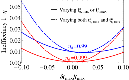
Figure 3: Inefficiency $1-\eta$ of the state transfer procedure as a function of relative variation of the maximum transmission amplitudes $\delta\textbf{t}_{\rm max}/\textbf{t}_{\rm max}=(\textbf{t}_{\rm e(r),max}^{\rm a}-\textbf{t}_{\rm e(r),max})/\textbf{t}_{\rm e(r),max}$ for design efficiencies $\eta_{\rm d}=0.99$ (blue curves) and $0.999$ (red curves). The maximum transmission amplitudes $\textbf{t}_{\rm e,max}$ and $\textbf{t}_{\rm r,max}$ are either varied simultaneously (dashed curves) or one of them is kept at the design value (solid curves). The superscript “a” indicates an “actual” value, different from the design value.

First, we assume that only the maximum amplitudes are inaccurate, $\textbf{t}_{\rm e,max}^{\rm a}=\textbf{t}_{\rm e,max}+\delta\textbf{t}_{\rm e,max}$ and $\textbf{t}_{\rm r,max}^{\rm a}=\textbf{t}_{\rm r,max}+\delta\textbf{t}_{\rm r,max}$, while other parameters are equal to their design values. (We change only the absolute values of $\textbf{t}_{\rm e,max}$ and $\textbf{t}_{\rm r,max}$, because their phases affect only the correctable final phase $\varphi_{\rm f}$ but do not affect the efficiency $\eta$.) In Fig. 3 we show the numerically calculated inefficiency $1-\eta$ of the state transfer as a function of the variation in maximum transmission amplitude $\delta\textbf{t}_{\rm max}/\textbf{t}_{\rm max}$, with the solid lines corresponding to variation of only one maximum amplitude, $\delta\textbf{t}_{\rm e,max}/\textbf{t}_{\rm e,max}$ or $\delta\textbf{t}_{\rm r,max}/\textbf{t}_{\rm r,max}$ (the results are the same), and the dashed lines corresponding to variation of both of them, $\delta\textbf{t}_{\rm e,max}/\textbf{t}_{\rm e,max}=\delta\textbf{t}_{\rm r,max}/\textbf{t}_{\rm r,max}$. The blue (upper) lines are for the case of design efficiency $\eta_{\rm d}=0.99$ and the red (lower) lines are for $\eta_{\rm d}=0.999$.

We see that deviations of the actual maximum amplitudes $\textbf{t}_{\rm e,max}^{\rm a}$ and $\textbf{t}_{\rm r,max}^{\rm a}$ from their design values $\textbf{t}_{\rm e,max}$ and $\textbf{t}_{\rm r,max}$ increase the inefficiency of the state transfer [essentially because of the inconsistency between $\textbf{t}_{\rm e(r),max}^{\rm a}$ and $\tau_{\rm e(r)}^{\rm a}$]. However, the effect is not very significant, with the additional inefficiency of less than 0.006 when one of the parameters deviates by $\pm 5\%$ and less than 0.02 when both of them deviate by $\pm 5\%$. The curves in Fig.  3 are approximately parabolic, with a growing asymmetry for larger $1-\eta_{\rm d}$.

For the case $\eta_{\rm d}\approx 1$ the numerical results for the additional inefficiency $-\delta\eta=\eta_{\rm d}-\eta$ can be approximately fitted by the formula

$$-\delta\eta\approx\left(\frac{\delta\textbf{t}_{\rm e,max}}{\textbf{t}_{\rm e,max}}\right)^{2}\!+\left(\frac{\delta\textbf{t}_{\rm r,max}}{\textbf{t}_{\rm r,max}}\right)^{2}\!+1.25\frac{\delta\textbf{t}_{\rm e,max}}{\textbf{t}_{\rm e,max}}\frac{\delta\textbf{t}_{\rm r,max}}{\textbf{t}_{\rm r,max}},$$ (34)

which we obtained by changing the maximum amplitudes symmetrically, antisymmetrically, and separately. Note that in the ideal procedure we assumed $|\textbf{t}_{\rm e,max}|=|\textbf{t}_{\rm r,max}|$.

The main result here is that the state transfer is quite robust against the small variation of the transmission amplitudes. We expect that experimentally these parameters can be calibrated with accuracy of a few per cent or better; the related inefficiency of the transfer protocol is very small.

III.2 Variation of buildup/leakage times $\tau_{\rm e}$ and $\tau_{\rm r}$

Now let us assume that in Eqs. (32) and (33) only the buildup/leakage time parameters are slightly inaccurate, $\tau_{\rm e}^{\rm a}=\tau+\delta\tau_{\rm e}$ and $\tau_{\rm r}^{\rm a}=\tau+\delta\tau_{\rm r}$ (we assume that in the ideal procedure $\tau_{\rm e}=\tau_{\rm r}=\tau$), while other parameters are equal to their design values. The transfer inefficiency as a function of the relative deviations $\delta\tau_{\rm e(r)}/\tau$ is shown in Fig. 4 for the design efficiencies $\eta_{\rm d}=0.99$ (blue lines) and $0.999$ (red lines). For the solid lines only one of the buildup/leakage times is varied (the results coincide), while for the dashed lines both parameters are varied together, $\delta\tau_{\rm e}=\delta\tau_{\rm r}$. As we see, $\pm 5\%$ variation of one of the buidup/leakage times increases the inefficiency by less than 0.001, and by less than 0.0025 if the both times are varied by $\pm 5\%$.

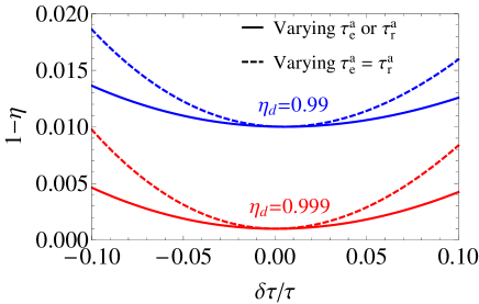
Figure 4: Dependence of the inefficiency $1-\eta$ on relative variation of the buildup/leakage time $\delta\tau_{\rm e(r)}/\tau=(\tau_{\rm e(r)}^{\rm a}-\tau)/\tau$ for design efficiencies $\eta_{\rm d}=0.99$ (blue curves) and $0.999$ (red curves), assuming $\tau_{\rm e}=\tau_{\rm r}=\tau$. The buildup/leakage times $\tau_{\rm e}^{\rm a}$ and $\tau_{\rm r}^{\rm a}$ are varied either simultaneously (dashed curves) or one of them is kept at the design value (solid curves).

The approximately parabolic dependences shown in Fig. 4 can be numerically fitted by the formula for the additional inefficiency $-\delta\eta$,

$$-\delta\eta\approx 0.34\left[\left(\frac{\delta\tau_{\rm e}}{\tau}\right)^{2}+\left(\frac{\delta\tau_{\rm r}}{\tau}\right)^{2}\right]+0.12\frac{\delta\tau_{\rm e}}{\tau}\frac{\delta\tau_{\rm r}}{\tau},$$ (35)

which was again obtained by varying $\delta\tau_{\rm e}$ and $\delta\tau_{\rm r}$ symmetrically, antisymmetrically, and separately. Most importantly, we see that the transfer procedure is robust against small deviations of the buildup/leakage times. (In an experiment we expect not more than a few per cent inaccuracy for these parameters.)

III.3 Variation of mid-times $t_{\rm m}^{\rm a,e}$ and $t_{\rm m}^{\rm a,r}$

Ideally, the pulse shapes $\textbf{t}_{\rm e}(t)$ and $\textbf{t}_{\rm r}(t)$ should switch from increasing/decreasing parts to constants at the same time $t_{\rm m}$, exactly in the middle of the procedure. However, due to imperfectly calibrated delays in the lines delivering the signals to the couplers, this change may occur at slightly different actual times $t_{\rm m}^{\rm a,e}$ and $t_{\rm m}^{\rm a,r}$, which are also not necessarily exactly in the middle of the procedure. Let us assume that $\textbf{t}_{\rm e}(t)$ and $\textbf{t}_{\rm r}(t)$ are given by Eqs. (32) and (33) with slightly inaccurate times $t_{\rm m}^{\rm a,e}$ and $t_{\rm m}^{\rm a,r}$, while other parameters are equal to their design values.

Solid lines in Fig. 5 show the dependence of the transfer inefficiency $1-\eta$ on the shift of the mid-time $\delta t_{\rm m}^{\rm r}=t_{\rm m}^{\rm a,r}-t_{\rm m}$, which is normalized by the buildup/leakage time $\tau$. Blue and red lines are for the design efficiencies $\eta_{\rm d}=0.99$ and 0.999, respectively. The case when only $t_{\rm m}^{\rm a,e}$ is changed is similar to what is shown by the solid lines up to the mirror symmetry, $\delta t_{\rm m}^{\rm r}\leftrightarrow-\delta t_{\rm m}^{\rm e}$. The dashed lines show the case when both mid-times are shifted simultaneously, $t_{\rm m}^{\rm a,e}=t_{\rm m}^{\rm a,r}$.

We see that when $t_{\rm m}^{\rm a,e}$ and $t_{\rm m}^{\rm a,r}$ coincide, there is practically no effect of the shift. This is because in this case the change is only due to slightly unequal durations $t_{\rm m}^{\rm a}$ and $t_{\rm f}-t_{\rm m}^{\rm a}$. A non-zero time mismatch $t_{\rm m}^{\rm a,e}-t_{\rm m}^{\rm a,r}$ has a much more serious effect because the reflection cancellation (13) becomes significantly degraded in the middle of the procedure, where the propagating field is at its maximum.

The numerical fit to a quadratic dependence gives

$$-\delta\eta\approx 0.25\left(\frac{\delta t_{\rm m}^{\rm a,e}-\delta t_{\rm m}^{\rm a,r}}{\tau}\right)^{2}.$$ (36)

For $\tau=33.3$ ns this means that $\sim$3 ns time mismatch leads to only $2\times 10^{-3}$ increase in inefficiency. Such robustness to the time mismatch is rather surprising. It can be qualitatively explained in the following way. The relative imperfection of the back-reflection cancellation (13) is approximately $(\delta t_{\rm m}^{\rm a,e}-\delta t_{\rm m}^{\rm a,r})/\tau$ in the middle of the procedure; however, the lost energy of the back-reflected field scales quadratically. Therefore, we can explain Eq. (36) up to a numerical factor. In an experiment we expect that the time mismatch can be made smaller than 1 ns; the corresponding inefficiency is almost negligible.

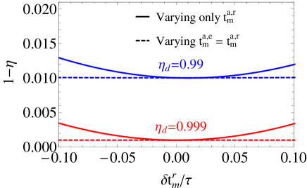
Figure 5: Inefficiency $1-\eta$ as a function of the mid-time shift $\delta t_{\rm m}^{\rm r}=t_{\rm m}^{\rm a,r}-t_{\rm m}$ normalized by the buildup/leakage time $\tau$. The mid-time $t_{\rm m}^{\rm a,e}$ is either varied equally (dashed curves) or kept constant (solid curves). The results for varying only $t_{\rm m}^{\rm a,e}$ are the same as the solid curves up to the sign change, $\delta t_{\rm m}^{\rm r}\leftrightarrow-\delta t_{\rm m}^{\rm e}$.

III.4 Pulse-shape warping

As another possible imperfection of the ideal time-dependences $\textbf{t}_{\rm e}(t)$ and $\textbf{t}_{\rm r}(t)$, we consider a nonlinear deformation (“warping”) with the form

$$\textbf{t}_{j}^{\rm a}(t)=\textbf{t}_{j}(t)\left[1+\alpha_{j}\frac{\textbf{t}_{j}(t)-\textbf{t}_{j,\rm max}}{\textbf{t}_{j,\rm max}}\right],\,\,\,j=\text{e,\,r},$$ (37)

where $\alpha_{\rm e}$ and $\alpha_{\rm r}$ are the warping parameters, which determine the strength of the deformations. Note that this deformation does not affect maximum values $\textbf{t}_{\rm e(r),max}$ and the values close to zero; it affects only intermediate values. The deformation imitates nonlinear (imperfectly compensated) conversion from experimental control signals into transmission amplitudes.

The inefficiency increase due to the warping of the transmission amplitude pulse shapes is illustrated in Fig. 6. Solid lines show the case when only $\alpha_{\rm e}$ or $\alpha_{\rm r}$ is non-zero (the results coincide), while the dashed lines show the case $\alpha_{\rm e}=\alpha_{\rm r}$. We see that for $\alpha_{\rm e}=\alpha_{\rm r}=0.05$ the inefficiency increases by $\sim 10^{-3}$ for both design efficiencies $\eta_{\rm d}=0.99$ and $0.999$. Similar to the variation of other parameters, the inefficiency due to the warping effect has a quadratic dependence on the warping parameters $\alpha_{\rm e}$ and $\alpha_{\rm r}$. The numerical fitting for small $|\alpha_{\rm e(r)}|$ and $\eta\approx 1$ gives

$$-\delta\eta\approx 0.22(\alpha_{\rm e}^{2}+\alpha_{\rm r}^{2})+0.12\alpha_{\rm e}\alpha_{\rm r}.$$ (38)

Again, this result shows that the state transfer is robust to distortion of the couplers’ transmission amplitude pulse shapes. We do not expect that uncompensated experimental nonlinearities will follow Eq. (37) exactly, since this equation only imitates a nonlinear conversion. However, very crudely, we would expect that $|\alpha_{\rm e(r)}|<0.05$ is a realistic experimental estimate.

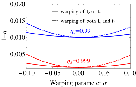
Figure 6: Dependence of the inefficiency $1-\eta$ on the warping parameters $\alpha_{\rm e}$ and $\alpha_{\rm r}$, introduced in Eq. (37) to describe the pulse shape distortion, for design efficiencies $\eta_{\rm d}=0.99$ (blue curves) and $0.999$ (red curves). The solid curves show the case when only one warping parameter is non-zero (the results coincide); the dashed curves are for the case $\alpha_{\rm e}=\alpha_{\rm r}$.

III.5 Smoothing by a Gaussian filter

In an actual experiment the designed pulse shapes for the transmission amplitudes of the tunable couplers given by Eqs. (22)–(25) will pass through a filter. Here we convolve the transmission amplitudes with a Gaussian function to simulate the experimental filtering, so the actual transmission amplitudes are

$$\textbf{t}_{j}^{\rm a}(t)=\frac{1}{\sqrt{2\pi}\,\sigma}\int_{-\infty}^{\infty}e^{-(t-t^{\prime})^{2}/2\sigma^{2}}\textbf{t}_{j}(t^{\prime})\,dt^{\prime},\,\,\,j=\text{e,\,r},\quad$$ (39)

where $\sigma$ is the time-width of the Gaussian filter. The filtering smooths out the kinks at the middle of the procedure and slightly lowers the initial and final values of $\textbf{t}_{\rm e}$ and $\textbf{t}_{\rm r}$. The change in transmission amplitudes translates into a decrease in the state transfer efficiency. Note that the smoothing reduces the energy loss at the beginning and end of the procedure, but causes an increased energy loss at the middle of the procedure, thus increasing the procedure inefficiency overall.

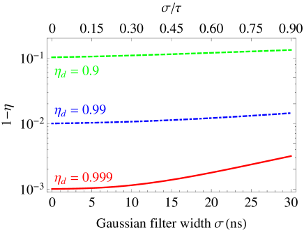
Figure 7: Inefficiency $1-\eta$ as a function of the width of a Gaussian filter $\sigma$ (in ns) for design efficiencies $\eta_{\rm d}=0.9$ (green dashed curve), $0.99$ (blue dot-dashed curve), and $0.999$ (red solid curve). We use $\tau=33.3\,\rm ns$, as in Fig. 2. The upper horizontal axis shows the normalized value $\sigma/\tau$.

The procedure inefficiency with the effect of the Gaussian filtering of transmission amplitudes is shown in Fig. 7 for the design efficiencies $\eta_{\rm d}=0.9$, $0.99$, and $0.999$. Rather surprisingly, the effect is very small, so that filtering with $\sigma=10$ ns does not produce a noticeable increase of the inefficiency, and even with $\sigma=30$ ns (which is close to the buildup/leakage time) the effect is still small. Such robustness to the filtering can be qualitatively understood in the same way as the robustness to the mismatch between the mid-times $\textbf{t}_{\rm e}(t)$ and $\textbf{t}_{\rm r}(t)$ discussed above. Note that experimentally Hofheinz-09 $\sigma$ is on the order of 1 ns, so the effect of the filter on the efficiency should be negligible.

III.6 Noisy transmission amplitudes

In experiment the pulse shapes $\textbf{t}_{\rm e}(t)$ and $\textbf{t}_{\rm r}(t)$ may contain noise. We model this noise by replacing the designed pulse shapes $\textbf{t}_{\rm e}(t)$ and $\textbf{t}_{\rm r}(t)$ with “actual” shapes as

$$\textbf{t}_{j}^{\rm a}(t)=\textbf{t}_{j}(t)[1+a\,\xi_{j}(t)],\,\,\,j=\text{e, r},$$ (40)

where $a$ corresponds to the dimensionless noise amplitude and $\xi_{\rm e}(t)$ and $\xi_{\rm r}(t)$ are mutually uncorrelated random processes. We generate each $\xi(t)$ numerically in the following way. First, we choose a time step $dt$ and generate $\xi(t)$ at discrete time moments $t=n\,dt$ (with integer $n$) as Gaussian-distributed random numbers with zero mean and unit standard deviation. After that we create a smooth function $\xi(t)$ passing through these points by polynomial interpolation. Since the noise contribution in Eq. (40) scales with the transmission amplitude $\textbf{t}_{j}$, we call it a multiplicative noise. Besides that, we also use a model of an additive noise defined as

$$\textbf{t}_{j}^{\rm a}(t)=\textbf{t}_{j}(t)+a\,\textbf{t}_{j,\rm max}\,\xi_{j}(t),\,\,\,j=\text{e,\,r},$$ (41)

where the relative amplitude $a$ is now compared with the maximum value $\textbf{t}_{j,\rm max}$, while each $\xi(t)$ is generated in the same way. Note that for sufficiently small $dt$ the noise $\xi(t)$ is practically white at low frequency; its variance $\overline{\xi^{2}}$ does not depend on $dt$, and therefore the low frequency spectral density is proportional to $dt$ (the effective cutoff frequency scales as $dt^{-1}$). Also note that the variance $\overline{\xi^{2}}$ somewhat depends on the method of interpolation used to generate $\xi(t)$. For the default interpolation method in Mathematica, which we used (polynomial interpolation of order three), $\overline{\xi^{2}}\approx 0.78$.

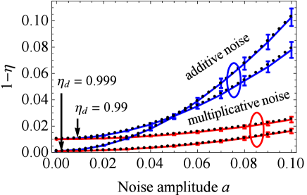
Figure 8: Solid lines: inefficiency $1-\eta$ averaged over 100 random noise realizations, as a function of the dimensionless noise amplitude $a$, for the multiplicative noise (red lines, bottom), Eq. (40), and the additive noise (blue lines, top), Eq. (41); both with $\overline{\xi^{2}}=0.78$. The error bars show the standard deviation for some values of $a$. The results are shown for $\eta_{\rm d}=0.99$ and $0.999$. In the simulation we used the time step $dt=1\,\rm ns$ and parameters of the procedure in Fig. 2 ($\tau=33.3\,\rm ns$). Black dotted lines (practically coinciding with the solid lines) are calculated by replacing the noise with the effective increase of the leakage rates $\kappa_{\rm e(r)}$ (see text).

The numerical results for the transfer inefficiency $1-\eta$ in the presence of noise are shown in Fig. 8 as a function of the dimensionless amplitude $a$. We used the time step $dt=1~{}\text{ns}$ and design efficiencies $\eta_{\rm d}=0.99$ and $\eta_{\rm d}=0.999$. The results are averaged over 100 random realizations; we show the average values by the solid lines and also show the standard deviations at some values of $a$. Red lines correspond to the multiplicative noise, while blue lines correspond to the additive noise. As expected, the additive noise leads to larger inefficiency than the multiplicative noise with the same amplitude, because of larger noise at the non-constant part of the pulse shape.

It is somewhat surprising that, as we checked numerically, the average results shown in Fig. 8 by the solid lines practically do not depend on the choice of the time step $dt$, as long as $dt\ll\tau_{\rm e(r)}$ (even though in our simulations $dt$ affects the noise spectral density). The error bars, however, scale with $dt$ as $\sqrt{dt}$. This behavior can be understood in the following way. In the evolution equations (1)–(3), the noise in $\textbf{t}_{\rm e}(t)$ and $\textbf{t}_{\rm r}(t)$ affects the leakage rates $\kappa_{\rm e}\propto|\textbf{t}_{\rm e}|^{2}$ and $\kappa_{\rm r}\propto|\textbf{t}_{\rm r}|^{2}$ of the two resonators, and also affects the transfer term $\sqrt{\kappa_{\rm e}\kappa_{\rm r}}\,A\propto|\textbf{t}_{\rm e}\textbf{t}_{\rm r}|$. On average the transfer term does not change (because the noises of $\textbf{t}_{\rm e}(t)$ and $\textbf{t}_{\rm r}(t)$ are uncorrelated); however, the average values of $|\textbf{t}_{\rm e}|^{2}$ and $|\textbf{t}_{\rm r}|^{2}$ change as $\langle|\textbf{t}_{\rm e(r)}^{\rm a}|^{2}\rangle=|\textbf{t}_{\rm e(r)}|^{2}(1+a^{2}\,\overline{\xi^{2}})$ for the model of Eq. (40) and as $\langle|\textbf{t}_{\rm e(r)}^{\rm a}|^{2}\rangle=|\textbf{t}_{\rm e(r)}|^{2}+a^{2}\,|\textbf{t}_{\rm e(r),max}|^{2}\,\overline{\xi^{2}}$ for the model of Eq. (41). Therefore, on average we expect dependence on $a^{2}\,\overline{\xi^{2}}$ (a second-order effect), but no dependence on $dt$, as long as it is sufficiently small. In contrast, the error bars in Fig. 8 should depend on $dt$ because the transfer term $\sqrt{\kappa_{\rm e}\kappa_{\rm r}}\,A$ fluctuates linearly in $\xi$. Since the low-frequency spectral density of $\xi(t)$ scales as $dt$, the typical fluctuation should scale as $\sqrt{dt}$, thus explaining such dependence for the error bars in Fig. 8. Simply speaking, for a wide-bandwith noise the average value of $1-\eta$ depends on the overall r.m.s. value of the noise, while the fluctuations of $1-\eta$ (from run to run) depend on the spectral density of the noise at relatively low frequencies ($\lesssim\tau^{-1}$). Note that the noise can increase or decrease the inefficiency compared to its average value; however, it always increases the inefficiency in comparison with the case without noise (as we see from Fig. 8, even if we increase $dt$ from 1 ns to about the buildup/leakage time of 33.3 ns, the error bars, increased by the factor $\sqrt{33.3}$, are still significantly less than the increase of inefficiency compared with the design value).

We have checked this explanation of the noise effect on the average inefficiency by replacing the fluctuating evolution equations (1)–(3) with non-fluctuating equations, in which the transfer term $\sqrt{\kappa_{\rm e}\kappa_{\rm r}}\,A$ does not change, while the leakage rates $\kappa_{\rm e}$ and $\kappa_{\rm r}$ are multiplied either by $1+a^{2}\,\overline{\xi^{2}}$ (for multiplicative noise) or by $1+a^{2}\,\overline{\xi^{2}}(\textbf{t}_{\rm e(r),max}/\textbf{t}_{\rm e(r)})^{2}$ for the additive noise. The results are shown in Fig. 8 by the dotted lines; we see that they almost coincide with the solid lines, thus confirming our explanation. We have also used several interpolation methods, which give somewhat different $\overline{\xi^{2}}$, and checked that the direct simulation with fluctuations and use of the non-fluctuating equations still give the same results.

As can be seen from Fig. 8, the average inefficiency depends approximately quadratically on the noise amplitude $a$ for both additive and multiplicative noise. The additional inefficiency $-\delta\eta$ can be fitted numerically as

$$-\delta\eta\approx c_{\rm n}a^{2}\,\overline{\xi^{2}},$$ (42)

where $c_{\rm n}\approx 2$ for the multiplicative noise and $c_{\rm n}\approx 2\,\ln\frac{1}{1-\eta_{\rm d}}$ for the additive noise. Note that for the additive noise $c_{\rm n}$ increases with decreasing design inefficiency $1-\eta_{\rm d}$, so the blue lines in Fig. 8 intersect. This is because a smaller $1-\eta_{\rm d}$ requires a longer procedure duration $t_{\rm f}$, causing more loss due to additional leakage of the resonators caused by fluctuating $\textbf{t}_{\rm e(r)}$.

The value of $c_{\rm n}$ for the additive noise can be derived analytically in the following way. As discussed above, the noise essentially increases the resonator leakages, $\kappa^{\rm a}_{\rm e(r)}(t)=\kappa_{\rm e(r)}(t)+a^{2}\,\overline{\xi^{2}}/\tau$, without increasing the transferred field; therefore, it is equivalent to the effect of energy relaxation with $T_{1}=\tau/(a^{2}\,\overline{\xi^{2}})$. Consequently (see below), the efficiency decreases as $\eta=\eta_{\rm d}\exp(-t_{\rm f}/T_{1})=\eta_{\rm d}\exp(-2a^{2}\,\overline{\xi^{2}}\ln\frac{1}{1-\eta_{\rm d}})$ [see Eq. (18) for $t_{\rm f}$], and the linear expansion of the exponent in this formula reproduces Eq. (42) with $c_{\rm n}=2\,\ln\frac{1}{1-\eta_{\rm d}}$.

The value of $c_{\rm n}$ for the multiplicative noise can be derived in a somewhat similar way. Now $\kappa^{\rm a}_{\rm e}(t)=\kappa_{\rm e}(t)(1+a^{2}\,\overline{\xi^{2}})$, so the additional leakage of the emitting resonator consumes the fraction $a^{2}\,\overline{\xi^{2}}$ of the transmitted energy. Using the time-reversal picture, we see that an analogous increase of the receiving resonator leakage, $\kappa^{\rm a}_{\rm r}(t)=\kappa_{\rm r}(t)(1+a^{2}\,\overline{\xi^{2}})$, emits (back-reflects) into the transmission line the fraction $a^{2}\,\overline{\xi^{2}}$ of the final energy $|B(t_{\rm f})|^{2}$. Combining these two losses, we obtain $\eta=\eta_{\rm d}(1-2a^{2}\,\overline{\xi^{2}})$, which for $\eta_{\rm d}\approx 1$ reproduces Eq. (42) with $c_{\rm n}=2$.

Overall, the efficiency decrease due to the multiplicative noise is not strong; for example, to keep $-\delta\eta<0.01$ we need the relative r.m.s. fluctuations of $\textbf{t}_{\rm e(r)}$ to be less than 7%. The (additive) fixed-amplitude fluctuations of $\textbf{t}_{\rm e(r)}$ can be more problematic, because the inability to keep $\textbf{t}_{\rm e(r)}$ near zero at the initial or final stage of the procedure leads to loss during most of the (relatively long) procedure. For example, for $\eta_{\rm d}=0.99$ and $-\delta\eta<0.01$, we need the r.m.s. fluctuations of $\textbf{t}_{\rm e(r)}$ to be less than 3% of $\textbf{t}_{\rm e(r),max}$.

III.7 Effect of dissipation

For completeness let us discuss here the effect of dissipation by assuming imperfect transfer through the transmission line, $\eta_{\rm tl}\neq 1$, and finite energy relaxation times $T_{1,\rm e}$ and $T_{1,\rm r}$ in the evolution equations (1)–(3), while the pulse shapes $\textbf{t}_{\rm e}(t)$ and $\textbf{t}_{\rm r}(t)$ are assumed to be ideal.

The effect of imperfect $\eta_{\rm tl}$ is easy to analyze, since the transmitted (classical) field is simply multiplied by $\sqrt{\eta_{\rm tl}}$. Therefore, the transfer procedure efficiency is simply multiplied by $\eta_{\rm tl}$, so that $\eta=\eta_{\rm tl}\eta_{\rm d}$. (Recall that we neglect multiple reflections.)

The effect of energy relaxation in the resonators is also very simple if $T_{1,\rm r}=T_{1,\rm e}=T_{1}$. Then the (classical) field decays equally everywhere, and therefore, after the procedure duration $t_{\rm f}$, the energy acquires the factor $\exp(-t_{\rm f}/T_{1})$, so that $\eta=\eta_{\rm d}\exp(-t_{\rm f}/T_{1})$. The analysis of the case when $T_{1,\rm r}\neq T_{1,\rm e}$ is not so obvious. We have analyzed this case numerically and found that the two resonators bring the factors $\exp(-t_{\rm f}/2T_{1,\rm e})$ and $\exp(-t_{\rm f}/2T_{1,\rm r})$, respectively.

Combining the effects of dissipation in the resonators and transmission line, we obtain

$$\eta=\eta_{\rm d}\eta_{\rm tl}\exp(-t_{\rm f}/2T_{1,\rm e})\exp(-t_{\rm f}/2T_{1,\rm r}),$$ (43)

assuming that everything else is ideal.

IV Multiple reflections

So far we have not considered multiple reflections of the field that is back-reflected from the receiving end, by assuming either a very long transmission line or the presence of a circulator [see Fig. 1(b)]. If there is no circulator and the transmission line is not very long (as for the state transfer between two on-chip superconducting resonators), then the back-reflected field bounces back and forth between the couplers and thus affects the efficiency of the state transfer. To describe these multiple reflections, we modify the field equations (1)–(3) by including the back-propagating field $F(t)$ into the dynamics, for simplicity assuming in this section $\Delta\omega_{\rm r}=\Delta\omega_{\rm e}=0$, $\eta_{\rm tl}=1$, and $T^{-1}_{1,\rm e(r)}=0$:

$$\dot{G}(t)=-\frac{\kappa_{\rm e}}{2}G(t)+\frac{\textbf{t}_{\rm e}}{|\textbf{t}_{\rm e}|}\frac{|\textbf{r}_{\rm e}|}{\textbf{r}_{\rm e}^{\rm in}}\sqrt{\kappa_{\rm e}}\,e^{i\varphi}F(t-t_{\rm d}),\qquad$$ (44)

$$\dot{B}(t)=-\frac{\kappa_{\rm r}}{2}B(t)+\frac{\textbf{t}_{\rm r}}{|\textbf{t}_{\rm r}|}\sqrt{\kappa_{\rm r}}A(t),$$ (45)

$$A(t)=\frac{\textbf{t}_{\rm e}}{|\textbf{t}_{\rm e}|}\sqrt{\kappa_{\rm e}}G(t)+\frac{\textbf{r}_{\rm e}^{\rm out}}{|\textbf{r}_{\rm e}|}e^{i\varphi}F(t-t_{\rm d}).$$ (46)

Here $t_{\rm d}$ is the round-trip delay time ($t_{\rm d}=2l_{\rm tl}/v$, where $l_{\rm tl}$ is the transmission line length and $v$ is the effective speed of light), $\varphi=\omega_{\rm e(r)}t_{\rm d}$ is the corresponding phase acquired in the round trip, $F(t)$ is given by Eq. (14), $\textbf{r}_{\rm e}^{\rm out}$ is the reflection amplitude of the emitting resonator coupler from the transmission line side, and $\textbf{r}_{\rm e}^{\rm in}$ is the same from the resonator side. Note that we use shifted clocks, so the propagation is formally infinitely fast in the forward direction and has velocity $v/2$ in the reverse direction; then the round-trip delay $t_{\rm d}$ and phase shift $\varphi$ are accumulated in the back-propagation only; the field $F(t)$ is defined at the receiving resonator, and it comes to the emitting resonator as $e^{i\varphi}F(t-t_{\rm d})$. Also note that even though $\varphi$ is proportional to $t_{\rm d}$, it is better to treat $\varphi$ as an independent parameter, because the time-delay effects are determined by the ratio $t_{\rm d}/\tau$, which has a very different scale from $\varphi=(t_{\rm d}/\tau)\,\omega_{\rm e(r)}\tau$, since $\omega_{\rm e(r)}\tau\sim 10^{3}$.

There is some asymmetry between Eqs. (44) and (45) and also between Eqs. (46) and (13), which involves factors $\textbf{r}^{\rm in}_{\rm e(r)}$. This is because in order to keep a simple form of the evolution equations (1)–(3), we essentially defined $G$ as the field propagating towards the transmission line, while $B$ propagates away from the transmission line. In this section we still assume that the phases of the transmission and reflection amplitudes ($\textbf{t}_{\rm e(r)}$ and $\textbf{r}_{\rm e(r)}^{\rm in(out)}$) do not change with time. For the tunable couplers of Refs. Yin13 ; Wen14 (see Appendix B) the transmission amplitudes $\textbf{t}_{\rm e(r)}$ are mostly imaginary, the reflection amplitudes $\textbf{r}_{\rm e(r)}^{\rm in}$ are close to $-1$, and $\textbf{r}_{\rm e(r)}^{\rm out}$ are somewhat close to $-1$ (recall that $\textbf{t}_{\rm e}^{2}/\textbf{r}_{\rm e}^{\rm in}\textbf{r}_{\rm e}^{\rm out}$ and $\textbf{t}_{\rm r}^{2}/\textbf{r}_{\rm r}^{\rm in}\textbf{r}_{\rm r}^{\rm out}$ must be real and negative from unitarity). In simulations it is easier to redefine the phases of the fields in the resonators and transmission line, so that $\textbf{t}_{\rm e}$ and $\textbf{t}_{\rm r}$ are treated as real and positive numbers, $\textbf{r}_{\rm e}^{\rm in}$ and $\textbf{r}_{\rm r}^{\rm in}$ are also real and positive (close to $1$), while $\textbf{r}_{\rm e}^{\rm out}$ and $\textbf{r}_{\rm r}^{\rm out}$ are real and negative (close to $-1$). In this case Eqs. (14) and (46) become $F=\sqrt{\kappa_{\rm r}}\,B-A$ and $A(t)=\sqrt{\kappa_{\rm e}}\,G(t)-e^{-i\varphi}F(t-t_{\rm d})$.

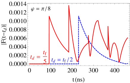
Figure 9: Illustration of the back-reflected field $|F(t-t_{\rm d})|$ reaching the emitting resonator at time $t$, for the round-trip delay time $t_{\rm d}=t_{\rm f}/2$ (blue dashed curve) and $t_{\rm d}=t_{\rm f}/5$ (red solid curve), assuming the round-trip phase shift $\varphi=\pi/8$. The kinks represent multiple reflections of the field emitted at $t=0$. We assumed parameters of Fig. 2 ($\eta_{\rm d}=0.999$, $\tau=33.3$ ns, $t_{\rm f}=460$ ns).

As an example of the dynamics with multiple reflections, in Fig. 9 we show the absolute value of the reflected field $F(t-t_{\rm d})$ (at the emitting resonator) for the procedure shown in Fig. 2 ($\eta_{\rm d}=0.999$, $t_{\rm f}=460$ ns) for the round-trip delays $t_{\rm d}=t_{\rm f}/2$ (blue dashed curve) and $t_{\rm d}=t_{\rm f}/5$ (red solid curve), assuming $\varphi=\pi/8$. The kinks represent the successive reflections of the field emitted at $t=0$. Note that depending on the phase shift $\varphi$, the resulting contribution of the reflected field into $B(t_{\rm f})$ can either increase or decrease $|B(t_{\rm f})|^{2}$, thus either decreasing or increasing the transfer efficiency $\eta$ (recall that the efficiency $\eta$ is defined disregarding the resulting phase $\varphi_{\rm f}$, because it can be easily corrected in an experiment). The effect of multiple reflections should vanish if $t_{\rm d}\geq t_{\rm f}$, i.e. when the transmission line is sufficiently long.

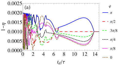
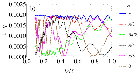
Figure 10: (a) Dependence of the inefficiency $1-\eta$ on the normalized delay $t_{\rm d}/\tau$ due to the round trip along the transmission line, for the design efficiency $\eta_{\rm d}=0.999$ and several values of the phase shift $\varphi$ accumulated in this round trip. The kinks at $t_{\rm d}/\tau=13.8/n$ correspond to the integer number $n$ of the round trips within the procedure time $t_{\rm f}$. (b) The same as in (a) for a smaller range of $t_{\rm d}/\tau$ (the results for $t_{\rm d}/\tau<0.1$ were not calculated). Notice that the inefficiency accounting for multiple reflections does not exceed twice the design inefficiency, $1-\eta\leq 2(1-\eta_{\rm d})$.

Figure 10 shows the numerically calculated inefficiency $1-\eta$ of the state transfer as a function of the round-trip delay time $t_{\rm d}$, normalized by the buildup/leakage time $\tau_{\rm e}=\tau_{\rm r}=\tau$. Different curves represent different values of the phase $\varphi$. The design efficiency is $\eta_{\rm d}=0.999$. (In the simulations we also used $\omega_{0}/2\pi=6$ GHz, and $\textbf{t}_{\rm e,max}=\textbf{t}_{\rm r,max}=0.05$; however, the presented results do not depend on these parameters). We see that the inefficiency shows an oscillatory behavior as a function of the delay time, but it is always within the range $0\leq 1-\eta\leq 2(1-\eta_{\rm d})$. This important fact was proved in Ref. Kor11 in the following way. In the case with the circulator, the losses are $1-\eta_{\rm d}=l_{G}^{\rm circ}+l_{F}^{\rm circ}$, where $l_{G}^{\rm circ}=|G^{\rm circ}(t_{\rm f})|^{2}$ is due to the untransmitted field [we assume here $G(0)=1$] and $l_{F}^{\rm circ}$ is the dimensionless energy carried away by the reflected field $F^{\rm circ}(t)$. In the case without circulator, we can simply add the multiple reflections of the field $F^{\rm circ}(t)$ to the evolution with the circulator. At the final time $t_{\rm f}$ the field $F^{\rm circ}(t)$ will linearly contribute to $B(t_{\rm f})$, $G(t_{\rm f})$, and the field within the transmission line [$F(t)$ for $t_{\rm f}-t_{\rm d}\leq t\leq t_{\rm f}$]. In the worst-case scenario the whole energy $l_{F}^{\rm circ}$ is added in-phase to the untransmitted field $G^{\rm circ}(t_{\rm f})$, resulting in $1-\eta=(\sqrt{l_{G}^{\rm circ}}+\sqrt{l_{F}^{\rm circ}})^{2}$. Since $(\sqrt{l_{G}^{\rm circ}}+\sqrt{l_{F}^{\rm circ}})^{2}\leq 2(l_{G}^{\rm circ}+l_{F}^{\rm circ})$ always, we obtain the upper bound for the inefficiency, $1-\eta\leq 2(1-\eta_{\rm d})$. The lower bound $1-\eta\geq 0$ is obvious. Figure 10 shows that both bounds can be reached (at least approximately) with multiple reflections at certain values of $t_{\rm d}/\tau$ and $\varphi$ (this fact is not obvious and is even somewhat surprising).

The dependence $\eta(t_{\rm d})$ shown in Fig. 10 is quite complicated and depends on the phase $\varphi$. We show only phases $0\leq\varphi\leq\pi$, while for $\pi\leq\varphi\leq 2\pi$ the results can be obtained from the symmetry $\eta(t_{\rm d},\varphi)=\eta(t_{\rm d},2\pi-\varphi)$. As we see from Fig. 10, the oscillations of $\eta(t_{\rm d})$ generally decrease in amplitude when $t_{\rm d}/\tau\rightarrow 0$, so that we expect a saturation of the dependence at $t_{\rm d}/\tau\rightarrow 0$. The exception is the case $\varphi=0$, when the oscillation amplitude does not significantly decrease at small $t_{\rm d}/\tau$ (numerical simulations become increasingly more difficult at smaller $t_{\rm d}/\tau$). This can be understood as due to the fact that for $\varphi=0$ the transmission line is a resonator, which is resonant with the frequency $\omega_{\rm e}=\omega_{\rm r}$ of the resonators.

Note that for an experiment with on-chip state transfer between superconducting resonators, the round-trip delay time $t_{\rm d}$ is comparable to $\omega_{\rm e(r)}^{-1}$ and therefore much smaller than $\tau$, $t_{\rm d}/\tau\sim 10^{-2}$. This regime is outside of the range accessible to our direct simulation method, which works well only when $t_{\rm d}/\tau\gtrsim 10^{-1}$. Nevertheless, we expect that the results presented in Fig. 10(b) can be approximately used in this case as well, because of the apparent saturation of $\eta(t_{\rm d})$ at $t_{\rm d}\rightarrow 0$, except when the phase $\varphi$ is close to zero.

The most important result of this section is that multiple reflections cannot increase the inefficiency $1-\eta$ by more than twice compared with the design inefficiency $1-\eta_{\rm d}$ (as obtained analytically and confirmed numerically).

V Mismatch of the resonator frequencies

The main idea of the state transfer protocol analyzed in this paper is to use destructive interference to suppress the back-reflection into the transmission line, thus providing a high-efficiency transfer. This is why it is crucial that the emitting and receiving resonators have almost the same frequency. Therefore, a mismatch between the two resonator frequencies should strongly decrease the transfer efficiency. In this section we analyze the effect of the frequency mismatch using two models. First, we assume a constant-in-time mismatch. Second, we consider the time-dependent detuning of the resonator frequencies due to the changing transmission amplitudes of the couplers, which lead to a changing complex phase of the reflection amplitudes (see Appendix B) and thus to the resonator frequency change.

V.1 Constant in time frequency mismatch

We first consider the case when the two resonator frequencies are slightly different, $\Delta\omega\equiv\omega_{\rm e}-\omega_{\rm r}\neq 0$, and they do not change in time. Everything else is assumed to be ideal. It is easy to understand the effect of detuning by using the evolution equations (1)–(3) and choosing $\omega_{0}=\omega_{r}$, so that $\Delta\omega_{\rm e}=\Delta\omega$ and $\Delta\omega_{\rm r}=0$. Then, compared with the case $\Delta\omega=0$, the emitting resonator field $G(t)$ acquires the phase factor $e^{-i\Delta\omega t}$; the same phase factor is acquired by the transmitted field $A(t)$ in Eq. (2), and this changing phase destroys the perfect phase synchronization between $A(t)$ and $B(t)$ that is needed to cancel the back-reflection.

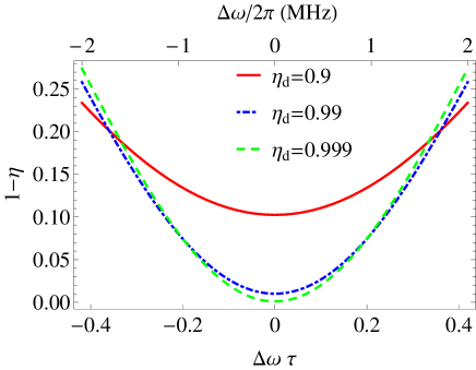
Figure 11: Inefficiency $1-\eta$ as a function of normalized detuning $\Delta\omega\,\tau$ (lower horizontal axis) for three design efficiencies, $\eta_{\rm d}=0.9,$ $0.99$, and $0.999$. The upper horizontal axis shows the unnormalized detuning $\Delta\omega/2\pi$ in MHz, using the values $\omega/2\pi=6$ GHz and $|\textbf{t}_{\rm e,max}|=|\textbf{t}_{\rm r,max}|=0.05$, so that $\tau=33.3$ ns.

The numerically calculated inefficiency $1-\eta$ is shown in Fig. 11 as a function of the detuning $\Delta\omega$, normalized by the inverse buildup/leakage time $\tau^{-1}$ (we assumed $\tau_{\rm e}=\tau_{\rm r}=\tau$). We show the lines for the design inefficiencies $\eta_{\rm d}=0.9$, 0.99, and 0.999. The results do not depend on $\omega_{\rm r}$ and $|\textbf{t}_{\rm e(r),max}|$. However, to express $\Delta\omega/2\pi$ in MHz on the upper horizontal axis, we use a particular example of $\omega_{\rm r}/2\pi=6$ GHz and $|\textbf{t}_{\rm e(r),max}|=0.05$, for which $\tau=33.3$ ns (as in Fig. 2).

For small $|\Delta\omega\,\tau|$ and $\eta_{\rm d}\approx 1$, the additional inefficiency due to frequency mismatch can be fitted as

$$-\delta\eta\approx c_{\rm fm}\,(\Delta\omega\,\tau)^{2},\,\,\,c_{\rm fm}\approx 2.$$ (47)

For smaller $\eta_{\rm d}$ the coefficient $c_{\rm fm}$ decreases, so that $c_{\rm fm}\approx 1.94$ for $\eta_{\rm d}=0.999$, $c_{\rm fm}\approx 1.68$ for $\eta_{\rm d}=0.99$, and $c_{\rm fm}\approx 0.81$ for $\eta_{\rm d}=0.9$.

It is interesting that the value $c_{\rm fm}=2$ for $\eta_{\rm d}\approx 1$ exactly coincides with the estimate derived in Ref. Kor11 , which we rederive here. Comparing the case $\Delta\omega\neq 0$ with the ideal case $\Delta\omega=0$, we can think that $A(t)$ acquires the extra phase factor $e^{-i\Delta\omega(t-t_{\rm m})}$, where $t_{\rm m}$ is the mid-time of the procedure (see Fig. 2); the overall factor $e^{i\Delta\omega t_{\rm m}}$ is not important, affecting only the final phase $\varphi_{\rm f}$. Then we can think that at $t=t_{\rm m}$ we still have an almost perfect cancellation of the back-reflection, $F(t_{\rm m})\approx 0$; however, at $t\neq t_{\rm m}$ the extra phase causes the back-reflected wave $|F(t)|\approx|A(t)(e^{-i\Delta\omega(t-t_{\rm m})}-1)|$. Now using $|A(t)|=|A(t_{\rm m})|e^{-|t-t_{\rm m}|/2\tau}$ and assuming $|\Delta\omega|\tau\ll 1$ (so that we can expand the exponent in the relevant time range), we find $|F(t)|\approx|A(t_{\rm m})|\,e^{-|t-t_{\rm m}|/2\tau}|\Delta\omega(t-t_{\rm m})|$. Finally integrating the loss, $\int|F(t)|^{2}dt$, and normalizing it by the transferred “energy” $\int|A(t_{\rm m})|^{2}e^{-|t-t_{\rm m}|/\tau}dt$, we obtain the added inefficiency $-\delta\eta\approx 2\,(\Delta\omega\,\tau)^{2}$.

Using this derivation, it is easy to understand why the coefficient $c_{\rm fm}$ in Eq. (47) decreases with decreasing $\eta_{\rm d}$. This occurs because the integration of $|F(t)|^{2}$ is limited by the range $0<t<t_{\rm f}=-2\tau\ln(1-\eta_{\rm d})$, which becomes shorter for smaller $\eta_{\rm d}$. Thus we can estimate $c_{\rm fm}$ as $c_{\rm fm}\approx\int_{0}^{-\ln(1-\eta_{\rm d})}x^{2}e^{-x}dx=2-(1-\eta_{\rm d})[2-2\ln(1-\eta_{\rm d})+\ln^{2}(1-\eta_{\rm d})]$, which fits the numerical results very well.

As expected, even small detuning significantly decreases the transfer efficiency. For example, to keep the added inefficiency under 1%, $-\delta\eta<0.01$, we need the detuning to be less than 0.4 MHz in the above example ($\tau=33.3$ ns), which is not very easy to achieve in an experiment.

V.2 Time-dependent detuning due to changing coupling

In an actual experimental coupler, the parameters are interrelated, and a change of the coupling strength by varying $|\textbf{t}|$ may lead to a change of other parameters. In particular, for the coupler realized experimentally in Refs. Yin13 ; Wen14 , the change of $|\textbf{t}|$ causes a small change of the complex phases of the transmission and reflection amplitudes t and $\textbf{r}^{\rm in(out)}$. The phase change of $\textbf{r}^{\rm in}$ (from the resonator side) causes a change of the resonator frequency. Thus, changing the coupling causes the frequency detuning, as was observed experimentally Yin13 . Since the frequency mismatch between the two resonators strongly decreases the efficiency of the state transfer, this is a serious problem for the protocol discussed in our paper. Here we analyze this effect quantitatively and discuss with which accuracy the detuning should be compensated (e.g. by another tunable element) to preserve the high-efficiency transfer.

Physically, the resonator frequency changes because the varying coupling changes the boundary condition at the end of the coplanar waveguide resonator (see Fig. 16 in Appendix B). Note that a somewhat similar frequency change due to changing coupling with a transmission line was studied in Ref. Goppl-08 .

As discussed in Appendix B, if we use the tunable couplers of Ref. Yin13 ; Wen14 , then the transmission and refection amplitudes $\textbf{t}_{j}$ and $\textbf{r}_{j}^{\rm in(out)}$ for the two resonators ($j=\rm e,\,r$) are given by the formulas

$$\textbf{t}_{j}=-i\frac{2\omega_{j}M_{j}}{1+b_{j}}\sqrt{\frac{R_{j}}{R_{\rm tl}}}\left(\frac{1}{R_{j}}+\frac{-ib_{j}}{\omega_{j}L_{e,j}}\right)\frac{1}{1-i\omega_{j}L_{2,j}/R_{\rm tl}},$$ (48)

$$\textbf{r}_{j}^{\rm in}=-\frac{1-b_{j}}{1+b_{j}},\,\,\,\textbf{r}_{j}^{\rm out}=-(\textbf{r}_{j}^{\rm in})^{*}\frac{\textbf{t}_{j}}{\textbf{t}_{j}^{*}},$$ (49)

where

$$b_{j}=\frac{i\omega L_{1,j}/R_{j}}{\displaystyle\frac{L_{1,j}}{L_{e,j}}+\left[1-\frac{i\omega_{j}M_{j}^{2}}{R_{\rm tl}L_{1,j}(1+i\omega_{j}L_{2,j}/R_{\rm tl})}\right]^{-1}},$$ (50)

$M_{j}$ is the effective mutual inductance in $j$th coupler (the main tunable parameter controlled by magnetic flux in the SQUID loop), $R_{j}$ and $R_{\rm tl}$ are the wave impedances of the resonators and the transmission line, $\omega_{j}$ are the resonator frequencies, and $L_{1,j}$, $L_{2,j}$, and $L_{e,j}$ are the effective inductances used to describe the coupler (see details in Appendix B). Note that Eqs. (48) and (50) are slightly different from the equations in the Supplementary Information of Ref. Yin13 and the derivation in Appendix B: the difference is that the imaginary unit $i$ is replaced with $-i$ to conform with the chosen rotating frame definition $e^{-i\omega t}$ in Eqs. (1) and (2).

For the typical experimental parameters, $|b_{j}|\ll 1$, so that $\textbf{r}_{j}^{\rm in}\approx-1$, while $\textbf{t}_{j}$ is mostly imaginary. Note that $\omega_{\rm e}\approx\omega_{\rm r}\approx\omega_{0}$, so in Eqs. (48) and (50) we can replace $\omega_{j}$ with $\omega_{0}$. Also note that there is no coupling, $\textbf{t}_{j}=0$, when $M_{j}=0$, and the coupling changes sign when $M_{j}$ crosses zero.

Tuning $M_{j}$, we control $|\textbf{t}_{j}|$. However, the complex phase of $\textbf{t}_{j}$ slightly changes with changing $M_{j}$ because $b_{j}$ in Eq. (48) depends on $M_{j}$ and also $L_{1,j}$ and $L_{2,j}$ depend on $M_{j}$ – see Appendix B. Changing the phase of $\textbf{t}_{j}$ leads to the phase mismatch in the state transfer protocol, degrading its efficiency. However, this is a relatively minor effect, while a much more serious effect is the dependence of the complex phase of $\textbf{r}_{j}^{\rm in}$ on $M_{j}$ via its dependence on $b_{j}$ in Eq. (49), leading to the resonator frequency change.

For the rotating frame $e^{-i\omega t}$ and quarter-wavelength resonator (which we assume here) the change $\delta(\arg\textbf{r}_{j}^{\rm in})$ of the phase of $\textbf{r}_{j}^{\rm in}$ changes the resonator frequency by

$$\delta\omega_{j}\approx-(\omega_{0}/\pi)\,\delta(\arg\textbf{r}_{j}^{\rm in}),$$ (51)

where we used $\omega_{j}\approx\omega_{0}$. Assuming for simplicity that the resonators are exactly on resonance ($\omega_{\rm e}=\omega_{\rm r}=\omega_{0}$) when there is no coupling ($M_{\rm e}=M_{\rm r}=0$), we can write the variable detunings to be used in the evolution equations (1) and (2) as

$$\Delta\omega_{j}=\omega_{j}-\omega_{0}=-\frac{\omega_{0}}{\pi}\left[\arg\textbf{r}_{j}^{\rm in}(M_{j})-\arg\textbf{r}_{j}^{\rm in}(0)\right],$$ (52)

where $\textbf{r}_{j}^{\rm in}(M_{j})$ describes dependence on $M_{j}$. Since $|\textbf{t}_{j}|$ also depends on $M_{j}$ (linearly to first approximation), we have an implicit dependence $\Delta\omega_{j}(|\textbf{t}_{j}|)$, which is linear for small $|\textbf{t}_{j}|$ [see Eq. (84) in Appendix B] and becomes nonlinear for larger $|\textbf{t}_{j}|$ .

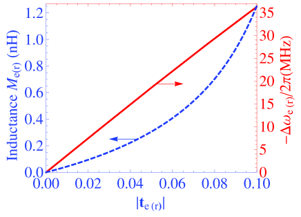
Figure 12: Red solid line: the resonator frequency detuning $-\Delta\omega_{\rm e(r)}/2\pi$ caused by changing $|\textbf{t}_{\rm e(r)}|$ for a particular set of parameters of the coupler (see text). Blue dashed line: the corresponding value of the coupler mutual inductance $M_{\rm e(r)}$. The arrows indicate the corresponding vertical axes.

This dependence $\Delta\omega_{\rm e(r)}(|\textbf{t}_{\rm e(r)}|)$ is shown in Fig. 12 by the solid line for the parameters of the coupler similar (though not equal) to the parameters of the experimental coupler Yin13 : $R_{\rm e(r)}=80\,\Omega$, $R_{\rm tl}=50\,\Omega$, $\omega_{0}/2\pi=6\,\rm GHz$, $L_{1,j}-M_{j}=L_{2,j}-M_{j}=620\,\rm pH$, and $L_{e,j}=180\,\rm pH$ (see Appendix B). In particular, Fig. 12 shows that $|\textbf{t}_{\rm e(r)}|=0.05$ corresponds to the frequency change by $-18.6$ MHz, which is a very big change compared to what is tolerable for a high-efficiency state transfer (see Fig. 11). The same detuning normalized by $\kappa_{\rm e(r)}=|\textbf{t}_{\rm e(r)}|^{2}\omega_{\rm e(r)}/\pi$ is shown in Fig.  13 by the dashed line.

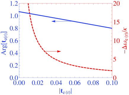
Figure 13: Solid line: the phase of the transmission amplitude, $\arg(\textbf{t}_{\rm e(r)})$, as a function of its absolute value $|\textbf{t}_{\rm e(r)}|$ for a particular set of coupler parameters (see text). Dashed line: the normalized detuning $-\Delta\omega_{\rm e(r)}/\kappa_{\rm e(r)}=-\pi\Delta\omega_{\rm e(r)}/\omega_{\rm e(r)}|\textbf{t}_{\rm e(r)}|^{2}$.

The value of $M_{\rm e(r)}$ needed to produce a given $|\textbf{t}_{\rm e(r)}|$ is shown in Fig. 12 by the dashed line. It is interesting that the dependence $M(|\textbf{t}|)$ is significantly more nonlinear than the dependence $\Delta\omega(|\textbf{t}|)$, indicating that the nonlinearities of $|\textbf{t}(M)|$ and $\Delta\omega(M)$ in Eqs. (48) and (52) partially cancel each other (see Appendix B).

The solid line in Fig. 13 shows dependence of the phase $\arg[\textbf{t}_{\rm e(r)}]$ on the absolute value $|\textbf{t}_{\rm e(r)}|$. Even though the phase change looks significant, it produces a relatively minor decrease in the protocol inefficiency (as we will see later) because the loss is quadratic in the phase mismatch.

We numerically simulate the state transfer protocol, accounting for the frequency change of the resonators and phase change of $\textbf{t}_{\rm e(r)}$ in the following way. First, we use the ideal pulse shapes $|\textbf{t}_{\rm e}(t)|$ and $|\textbf{t}_{\rm r}(t)|$ from Eqs. (22)–(25), assuming a symmetric setup ($\tau_{\rm e}=\tau_{\rm r}$). Then we calculate the corresponding dependences $M_{\rm e}(t)$ and $M_{\rm r}(t)$ using Eq. (48) and find $\textbf{t}_{\rm e}(t)$ and $\textbf{t}_{\rm r}(t)$ (now with time-dependent phases) using the same Eq. (48), and also find the detunings $\Delta\omega_{\rm e}(t)$ and $\Delta\omega_{\rm r}(t)$ using Eq. (52). After that we solve the evolution equations (1)–(3), neglecting multiple reflections. Note that we convert $|\textbf{t}_{j}(t)|$ into $M_{j}(t)$ by first numerically calculating $|\textbf{t}_{j}(M_{j})|$ from Eq. (48), then fitting the inverse dependence $M_{j}(|\textbf{t}_{j}|)$ with a polynomial of 40th order, and then using this polynomial for the conversion.

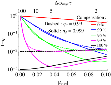
Figure 14: Inefficiency $1-\eta$ as a function of $|\textbf{t}_{\rm e,max}|=|\textbf{t}_{\rm r,max}|$ for the couplers with parameters described in the text. The solid lines are for the design efficiency $\eta_{\rm d}=0.999$, while the dashed lines are for $\eta_{\rm d}=0.99$. The red lines show the results without compensation of the frequency detuning $\Delta\omega_{\rm e(r)}(t)$ caused by changing $|\textbf{t}_{\rm e(r)}(t)|$ and correspondingly changing $\arg(\textbf{r}_{\rm e(t)}^{\rm in})$. The blue lines assume 90% compensation of this detuning, 95% compensation for the green lines, 99% compensation for the magenta lines, and full 100% compensation for the black lines. For the black lines the extra inefficiency is caused only by changing phases of $\textbf{t}_{\rm e(r)}$. The upper horizontal axis shows the product $\Delta\omega_{\rm max}\,\tau$, corresponding to $|\textbf{t}_{\rm max}|$.

Figure 14 shows the numerically calculated inefficiency $1-\eta$ of the transfer protocol as a function of the maximum transmission amplitude $|\textbf{t}_{\rm e,max}|=|\textbf{t}_{\rm r,max}|$ for the above example of the coupler parameters and design efficiencies $\eta_{\rm d}=0.99$ and 0.999. Besides showing the results for the usual protocol (red lines), we also show the results for the cases when the frequency detuning [Eq. (52)] is reduced by a factor of 10 (90% compensation, blue lines), 20 (95% compensation, green lines), 100 (99% compensation, magenta lines) and fully eliminated (100% compensation, black lines). Such compensation can be done experimentally by using another circuit element, affecting the resonator frequency, e.g., tuning the phase of the reflection amplitude at the other end of the resonator by a SQUID-controlled inductance.

We see that without compensation of the frequency detuning the state transfer protocol cannot provide a high efficiency: $\eta=0.33$ for $|\textbf{t}_{\rm max}|=0.05$ and $\eta=0.58$ for $|\textbf{t}_{\rm max}|=0.1$. However, with the detuning compensation the high efficiency may be restored. As we see from Fig. 14, the state transfer efficiency above 99% requires the detuning compensation at least within 90%–95% range (depending on $|\textbf{t}_{\rm max}|$). Note that even with 100% compensation, the efficiency is less than in the ideal case. This is because of the changing phases of $\textbf{t}_{\rm e}(t)$ and $\textbf{t}_{\rm r}(t)$. However, this effect is minor in comparison with the effect of detuning.

It is interesting that the curves in Fig. 14 decrease with increasing $|\textbf{t}_{\rm max}|$ when $|\textbf{t}_{\rm max}|$ is not too large. This may seem counterintuitive, since larger $|\textbf{t}|$ leads to larger detuning, and so we would naively expect larger inefficiency at larger $|\textbf{t}_{\rm max}|$. The numerical result is opposite because the duration of the procedure decreases, scaling as $\tau\propto|\textbf{t}_{\rm max}|^{-2}$. Therefore if the largest detuning scales linearly, $|\Delta\omega_{\rm max}|\propto|\textbf{t}_{\rm max}|$, then the figure of merit $|\Delta\omega_{\rm max}\tau|$ scales as $|\textbf{t}_{\rm max}|^{-1}$, thus explaining the decreasing part of the curves in Fig. 14. The upper horizontal axis in Fig. 14 shows $|\Delta\omega_{\rm max}\tau|$, which indeed decreases with increasing $|\textbf{t}_{\rm max}|$ (see also the dashed line in Fig. 13).

More quantitatively, let us assume a linear detuning, $\Delta\omega_{\rm e(r)}=k\,|\textbf{t}_{\rm e(r)}|$, where the coefficient $k$ is given by Eq. (84) multiplied by the uncompensated fraction of the detuning. Assuming a small deviation from the ideal protocol, the transmitted wave is $|A(t)|=|A(t_{m})|\,e^{-|\Delta t|/2\tau}$, where $\Delta t=t-t_{\rm m}$. At the mid-time $t_{\rm m}$ the resonator frequencies coincide, but at $t>t_{\rm m}$ the receiving resonator frequency changes so that $\Delta\omega=\omega_{\rm e}-\omega_{\rm r}=k(|\textbf{t}_{\rm r}(t_{\rm m})|-|\textbf{t}_{\rm r}(t)|)$. Using Eq. (24) we find $\Delta\omega=k\,|\textbf{t}_{\rm max}|\,[1-(2e^{\Delta t/\tau}-1)^{-1/2}]$. The accumulated phase mismatch is then $\phi(t)=\int_{t_{m}}^{t}\Delta\omega(t^{\prime})\,dt^{\prime}$, which produces the reflected wave $|F|\approx|A\phi|$, assuming small $\phi$. The inefficiency due to the reflected wave loss is then $1-\eta\approx\int_{t_{m}}^{\infty}|F(t)|^{2}\,dt/\int_{t_{m}}^{\infty}|A(t)|^{2}\,dt$ (note that due to symmetry the same relative loss is before and after $t_{\rm m}$). Therefore $1-\eta\approx\tau^{-1}k^{2}|\textbf{t}_{\rm max}|^{2}\int_{0}^{\infty}\{\int_{0}^{x}[1-(2e^{\Delta t/\tau}-1)^{-1/2}]\,d\Delta t\}^{2}e^{-x/\tau}dx$, and calculating the integral numerically we obtain $1-\eta=0.63\,k^{2}\tau^{2}|\textbf{t}_{\rm max}|^{2}$ [the numerical value of the integral is somewhat smaller than 0.63 if we limit the outer integration by $-\tau\ln(1-\eta_{\rm d})$]. Finally using $\tau=\pi/\omega_{0}|\textbf{t}_{\rm max}|^{2}$, we obtain $1-\eta\approx 0.6\,(k\pi/\omega_{0}|\textbf{t}_{\rm max}|)^{2}$.

Numerical results in Fig. 14 reproduce the scaling $1-\nobreak\eta\propto(k/|\textbf{t}_{\rm max}|)^{2}$ for the significant part of the curves for $\eta_{\rm d}=0.999$ (when plotted in log-log scale); however, the prefactor in the numerical fitting is somewhat different from what we obtained above: $1-\eta\approx 0.4\,(k\pi/\omega_{0}|\textbf{t}_{\rm max}|)^{2}$. Note that at sufficiently large $|\textbf{t}_{\rm max}|$ the green and red curves in Fig. 14 reach a minimum and then start to increase. This occurs because the inefficiency due to changing phase of $\textbf{t}_{\rm e(r)}$ increases with increasing $|\textbf{t}_{\rm max}|$, in contrast to the effect of frequency detuning.

Actually, our analysis of the transfer process in the case of complete compensation of detuning is not fully accurate. The reason is that in the evolution equations (1)–(3) we took into account the frequency change due to changing $\textbf{r}^{\rm in}_{\rm e(r)}$, but we did not take into account another (very small) effect due to changing $\textbf{r}^{\rm in}_{\rm e(r)}$. It is easy to understand the origin of this effect in the following way. There is a phase difference $\arg(\textbf{r}^{\rm in}_{\rm r})$ between the field $B$ propagating away from the transmission line and the similar field propagating towards the transmission line [see Eq.  (13) and discussion below it]. Changing $\arg(\textbf{r}^{\rm in}_{\rm r})$ alters this phase difference, thus affecting both fields and correspondingly leading to an extra term, neglected in Eq. (2). Similarly, changing $\arg(\textbf{r}^{\rm in}_{\rm e})$ leads to an extra term in Eq. (1) for $G$. However, as can be seen from Fig. 12 and Eq. (51), the change of $\arg(\textbf{r}^{\rm in}_{\rm e(r)})$ is less than 0.02 for $|\textbf{t}_{\rm e(r)}|$ varying between 0 and 0.1, which is much less than the change of $\arg(\textbf{t}_{\rm e(r)})$ in Fig. 13. Therefore, the neglected effect is much less than the effect due to changing $\arg(\textbf{t}_{\rm e(r)})$, which by itself is almost negligible, as seen in Fig. 14. Note that the compensation for changing phases can be done experimentally in the same way as the compensation for the detuning, so that in principle the efficiency decrease analyzed in this section can be fully avoided.

Overall, we see that the detuning of the resonator frequencies due to a changing coupling is a serious problem for the state transfer protocol. A high-efficiency state transfer is possible only with additional experimental effort to compensate for this detuning. The required compensation accuracy is crudely within 90%–95% range. The use of a shorter protocol (by using a stronger coupling) helps to increase the efficiency. Note that the frequency compensation is done routinely for the tunable coupler of Refs. Hoffman-11 ; Sri14 ; similarly, the phase compensation can be naturally realized in the tunable coupler of Refs. Pechal2014 ; Zeytinoglu2015 .

VI Conclusion

In this paper we have analyzed the robustness of the quantum state transfer protocol of Ref. Kor11 for the transfer between two superconducting resonators via a transmission line. The protocol is based on destructive interference, which cancels the back-reflection of the field into the transmission line at the receiving end (we believe this explanation is more natural than the terminology of time reversal, introduced in Ref. Cir97 ). This is achieved by using tunable couplers for both resonators and properly designed time-dependences (pulse shapes) of the transmission amplitudes $\textbf{t}_{\rm e}(t)$ and $\textbf{t}_{\rm r}(t)$ for these couplers. Nearly-perfect transfer efficiency $\eta$ can be achieved in the ideal case. We have focused on analyzing additional inefficiency due to deviations from the ideal case.

The ideal pulse shapes of the transmission amplitudes [Eqs. (22)–(25)] depend on several parameters; we have studied additional inefficiency due to deviations of these parameters from their design values. Below, we summarize our results by presenting the tolerable deviations for a fixed additional inefficiency of $-\delta\eta=0.01$ (because of quadratic scaling, the tolerable inaccuracies for $-\delta\eta=0.001$ are about 3.2 times smaller). For the relative deviations of the maximum transmission amplitudes $|\textbf{t}_{\rm e,max}|$ and $|\textbf{t}_{\rm r,max}|$, the tolerable ranges are $\pm 10\%$ if only one of them is changing and $\pm 5\%$ if both of them are changing simultaneously [see Fig. 3 and Eq. (34)]. For the relative deviations of the time scale parameters $\tau_{\rm e}$ and $\tau_{\rm r}$ describing the exponential increase/decrease of the transmitted field, the tolerable ranges are $\pm 17\%$ if only one of them is changing and $\pm 11\%$ if both of them are changing simultaneously [see Fig. 4 and Eq. (35)]. For the mismatch between the mid-times $t_{\rm m}$ of the procedure in the two couplers, the tolerable range is $\pm 0.2\tau\simeq\pm 6$ ns [see Fig. 5 and Eq. (36)]. For a nonlinear distortion described by warping parameters $\alpha_{\rm e}$ and $\alpha_{\rm r}$ [see Eq. (37)], the tolerable parameter range is $\pm 0.2$ if the distortion affects only one coupler and $\pm 0.13$ if the distortion affects both couplers. Our results show that smoothing of the pulse shapes by a Gaussian filter practically does not affect the inefficiency; even filtering with the width $\sigma\simeq\tau\simeq 30$ ns is still tolerable. When the pulse shapes are distorted by an additional (relatively high-frequency) noise, the tolerable range for the standard deviation of $|\textbf{t}_{\rm e(r)}|$ is 7% of the instantaneous value and 3% of the maximum value [see Fig. 8 and Eq. (42)]. Overall, we see that the state transfer procedure is surprisingly robust to various distortions of the pulse shapes.

We have also analyzed the effect of multiple reflections and found that it can both increase or decrease the transfer efficiency. However, even in the worst case, this effect cannot increase the inefficiency $1-\eta$ by more than a factor of 2 (see Fig. 10). The energy dissipation in the transmission line or in the resonators can be a serious problem for the state transfer protocol. The description of the effect is simple [see Eq. (43)]; for a high-efficiency transfer we can tolerate only a weak dissipation $1-\eta_{\rm tl}$ in the transmission line, and we also need the procedure duration $t_{\rm f}$ to be much shorter than the energy relaxation time $T_{1}$. In particular, for $-\delta\eta=0.01$ we need $\eta_{\rm tl}>0.99$ and $T_{1}>100\,t_{\rm f}$.

The major problem in realizing the state transfer protocol is the frequency mismatch between the two resonators, since the destructive interference is very sensitive to the frequency mismatch. For a fixed detuning, the tolerable frequency mismatch $(\omega_{\rm e}-\omega_{\rm r})/2\pi$ for $-\delta\eta=0.01$ is only $\pm 0.01/\tau\simeq\pm 0.4$ MHz [see Fig. 11 and Eq. (47)]; the tolerable range is a factor of $\sqrt{10}$ smaller for $-\delta\eta=0.001$. An even more serious problem is the change of the resonator frequencies caused by changing couplings, which for the coupler of Ref. Yin13 is on the order of 20 MHz [see Fig. 12 and Eq. (84) in Appendix B]. Without active compensation for this frequency change, a high-efficiency state transfer is impossible. Our numerical results show (see Fig. 14) that to realize efficiency $\eta=0.99$, the accuracy of the compensation should be at least 90% (i.e., the frequency change should be decreased by an order of magnitude). It is somewhat counterintuitive that a better efficiency can be obtained by using a higher maximum coupling, which increases the frequency mismatch but decreases duration of the procedure (see Fig. 14). Another effect that decreases the efficiency is the change of the phase of the transmission amplitude with changing coupling. However, this effect produces a relatively minor decrease of the efficiency (see Fig. 14).

In most of the paper we have considered a classical state transfer, characterized by the (energy) efficiency $\eta$. However, all the results have direct relation to the transfer of a quantum state (see Appendix A). In particular, for a qubit state transfer, the quantum process fidelity $F_{\chi}$ is $F_{\chi}\approx 1-(1-\eta)/2$ for $\eta\approx 1$ [see Eq. (12)].

The quantum state transfer protocol analyzed in this paper has already been partially realized experimentally. In particular, the realization of the proper (exponentially increasing) waveform for the quantum signal emitted from a qubit has been demonstrated in Ref. Sri14 (a reliable frequency compensation has also been demonstrated in that paper). The capture of such a waveform with 99.4% efficiency has been demonstrated in Ref. Wen14 . We hope that the full protocol that combines these two parts will be realized in the near future.

Appendix A Quantum state transfer using the beam splitter theory

In this Appendix we discuss the quantum theory of state transfer using the optical language of beam splitters. The starting point is Eq. (7), in which the resulting classical field $B(t_{\rm f})$ has the contribution $\sqrt{\eta}\,e^{i\varphi_{\rm f}}G(0)$ from the transferred field $G(0)$ and also contributions from other fields. This equation describes a unitary transformation, which can be modeled as a result of adding the (infinite number of) fields [$B(0)$ and time-binned $V(t)$] by using a system of (infinite number of) beam splitters. Then using linearity of the evolution, we can simply replace the classical fields with the corresponding annihilation operators for quantum fields, thus developing the quantum theory of the state transfer.

In the case when all other fields in Eq. (7) except $G(0)$ correspond to vacuum, it is sufficient to consider one beam splitter because a linear combination of vacua is still vacuum. This is why in this Appendix we mainly discuss one beam splitter (characterized by the amplitude $\sqrt{\eta}$ and phase $\varphi_{\rm f}$ in the main path), with the initial state to be transferred at one arm and vacuum state at the other arm. Note that notations in this Appendix are different from the notations in the main text.

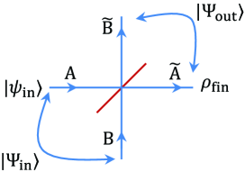
Figure 15: A beam splitter with input classical fields $A$ and $B$ transformed into the output fields $\tilde{A}$ and $\tilde{B}$, with the main transformation $A\rightarrow\tilde{A}$ characterized by the amplitude $\sqrt{\eta}$ and phase shift $\varphi_{\rm f}$. In the quantum formulation the input state $|\Psi_{\rm in}\rangle$ is transformed into the output state $|\Psi_{\rm out}\rangle$. In particular, in Sec. A.1 we consider the input state $|\Psi_{\rm in}\rangle=|\psi_{\rm in}\rangle|0\rangle$, calculate $|\Psi_{\rm out}\rangle$, and then reduce it to the density matrix $\rho_{\rm fin}$ of the main output arm, by tracing over the other output arm.

Let us start with revisiting the quantum theory of a beam splitter Ger06 (Fig. 15). The quantum theory follows the classical description of the beam splitter, which is characterized by the following relations between the input classical fields $A$ and $B$, and the output classical fields $\tilde{A}$ and $\tilde{B}$:

$$\tilde{A}=\sqrt{\eta}\,e^{i\varphi_{1}}A+\sqrt{1-\eta}\,e^{i\varphi_{2}}B,$$ (53)

$$\tilde{B}=\sqrt{\eta}\,e^{i\varphi_{3}}B-\sqrt{1-\eta}\,e^{i(\varphi_{1}-\varphi_{2}+\varphi_{3})}A,$$ (54)

where $\varphi_{1}=\varphi_{\rm f}$ and other phases are introduced to describe a general unitary transformation (these phases can include phase shifts in all four arms). Exactly the same relations also apply in the quantum case for the annihilation operators $\tilde{a}$ and $\tilde{b}$ of the fields at the output arms and the annihilation operators $a$ and $b$ of the fields at the input arms.

In general, we want to find an output quantum state $|\Psi_{\rm out}\rangle$ for a given input state $|\Psi_{\rm in}\rangle$, which in principle can be an entangled state of the two input modes. This can be done Ger06 by applying the following steps:

1. Express the input state $|\Psi_{\rm in}\rangle$ in terms of the input creation operators $a^{\dagger}$ and $b^{\dagger}$, and vacuum.

2. Using Eqs. (53) and (54), express $A$ and $B$ via $\tilde{A}$ and $\tilde{B}$. These are the equations expressing $a$ and $b$ in terms of $\tilde{a}$ and $\tilde{b}$. Conjugate these equations to express $a^{\dagger}$ and $b^{\dagger}$ in terms of $\tilde{a}^{\dagger}$ and $\tilde{b}^{\dagger}$.

3. Substitute the operators $a^{\dagger}$ and $b^{\dagger}$ used in the step 1 by their expressions in terms of $\tilde{a}^{\dagger}$ and $\tilde{b}^{\dagger}$ obtained in step 2. This substitution gives $|\Psi_{\rm out}\rangle$.

Now let us apply this substitution method to find the resulting state in the receiving resonator when an arbitrary quantum state is transferred from the emitting resonator.

A.1 Transfer of an arbitrary quantum state

Let us assume that the initial state $|\psi_{\rm in}\rangle$ in the emitting resonator is

$$|\psi_{\rm in}\rangle=\sum_{n}\alpha_{n}|n\rangle=\sum_{n}\frac{\alpha_{n}(a^{\dagger})^{n}}{\sqrt{n!}}|0\rangle,\,\,\,\sum_{n}|\alpha_{n}|^{2}=1,$$ (55)

while all other fields involved in the transfer procedure are vacua (in particular, this assumes zero temperature). Then the two-arm input state $|\Psi_{\rm in}\rangle$ for the beam splitter is the same, except the vacuum $|0\rangle$ in Eq. (55) is now understood as the vacuum $|\bf{0}\rangle$ for all possible modes.

The transfer procedure is characterized only by the efficiency $\eta$ and the phase $\varphi_{\rm f}=\varphi_{1}$, while other phases $\varphi_{2}$ and $\varphi_{3}$ in Eqs. (53) and (54) are undefined. However, even though the resulting state $|\Psi_{\rm out}\rangle$ will depend on $\varphi_{2}$ and $\varphi_{3}$, the resulting density matrix $\rho_{\rm fin}$, obtained from $|\Psi_{\rm out}\rangle$ by tracing over the other output arm, will not depend on $\varphi_{2}$ and $\varphi_{3}$. This is because arbitrary $\varphi_{2}$ and $\varphi_{3}$ can be produced by placing phase shifters in the ancillary input and output arms ($B$-arm and $\tilde{B}$-arm in Fig. 15); shifting the phase of vacuum in the $B$-arm does not produce any effect, while shifting the phase in the $\tilde{B}$-arm cannot affect $\rho_{\rm fin}$ by causality. We have also checked independence of $\rho_{\rm fin}$ on $\varphi_{2}$ and $\varphi_{3}$ by explicit calculations. Therefore, we can choose any values of $\varphi_{2}$ and $\varphi_{3}$. For convenience, let us choose $\varphi_{2}=\pi$ and $\varphi_{3}=0$. Then using step 2 of the substitution method we obtain

$$a^{\dagger}=\sqrt{\eta}\,e^{i\varphi_{\rm f}}\tilde{a}^{\dagger}+\sqrt{1-\eta}\,e^{i\varphi_{\rm f}}\tilde{b}^{\dagger},$$ (56)

$$b^{\dagger}=\sqrt{\eta}\,\tilde{b}^{\dagger}-\sqrt{1-\eta}\,\tilde{a}^{\dagger},$$ (57)

while step 1 was Eq. (55). Now substituting $a^{\dagger}$ in Eq. (55) with the expression in Eq. (56) (step 3), we obtain

$$|\Psi_{\rm out}\rangle =\sum_{n,k}\alpha_{n+k}\sqrt{(n+k)!/(n!k!)}\,\eta^{n/2}(1-\eta)^{k/2}$$

$$\times e^{i(n+k)\varphi_{\rm f}}|n\rangle|k\rangle,$$ (58)

where in the notation $|n\rangle|k\rangle=[(\tilde{a}^{\dagger})^{n}(\tilde{b}^{\dagger})^{k}/\sqrt{n!k!}\,]\,|{\bf 0}\rangle$ the second state corresponds to the ancillary second arm (upper arm in Fig. 15).

The final state at the receiving resonator can be calculated by tracing $|\Psi_{\rm out}\rangle\langle\Psi_{\rm out}|$ over the ancillary state $|k\rangle$, thus obtaining the density matrix

$$\rho_{\rm fin} =\sum_{j,n,m}\alpha_{n+j}\alpha^{*}_{m+j}\sqrt{(n+j)!(m+j)!}/(j!\sqrt{n!m!})$$

$$\hskip 22.76228pt\times\eta^{(n+m)/2}(1-\eta)^{j}e^{i(n-m)\varphi_{\rm f}})\,|n\rangle\langle m|,\quad$$ (59)

where the sums over $j$, $n$, and $m$ are all from 0 to $\infty$. Note that this result has been derived for a pure initial state (55) in the emitting resonator. However, it is easy to generalize Eq. (59) to an arbitrary initial state $\rho_{\rm in}$ by replacing $\alpha_{n+j}\alpha^{*}_{m+j}$ with $(\rho_{\rm in})_{n+j,m+j}$.

To find the fidelity of the quantum state transfer for the initial state (55), we calculate the overlap $\langle\psi_{\rm in}|\rho_{\rm fin}|\psi_{\rm in}\rangle$, thus obtaining

$$F_{\rm st} =\sum_{j,n,m}\frac{\sqrt{(n+j)!(m+j)!}}{j!\sqrt{n!m!}}\,\alpha_{n}^{*}\alpha_{m}\alpha_{n+j}\alpha^{*}_{m+j}$$

$$\hskip 25.6073pt\times\eta^{(n+m)/2}(1-\eta)^{j}e^{i(n-m)\varphi_{\rm f}},$$ (60)

which is Eq. (9) in the main text. For a mixed input state $\rho_{\rm in}$ we can find the resulting state $\rho_{\rm fin}$ as discussed above and then use the Uhlmann fidelity definition N-C-book $F_{\rm st}=[\mbox{Tr}\sqrt{\sqrt{\rho_{\rm in}}\,\rho_{\rm fin}\sqrt{\rho_{\rm in}}}]^{2}$.

If instead of an arbitrary state (55) we transfer a qubit state $|\psi_{\rm in}\rangle=\alpha_{0}|0\rangle+\alpha_{1}|1\rangle$, then in Eq. (58) there are only three terms because $\alpha_{n+k}=0$ if $n+k>1$. This reduces Eq. (58) to Eq. (10) in the main text. Similarly, Eq. (59) reduces to Eq. (11) and Eq. (60) reduces to

$$F_{\rm st}=|\alpha_{0}|^{4}+\eta|\alpha_{1}|^{2}+|\alpha_{0}|^{2}|\alpha_{1}|^{2}(1-\eta+2\sqrt{\eta}\cos\varphi_{\rm f}).$$ (61)

To average this fidelity over the Bloch sphere of the initial state, we can either average it over 6 points at the ends of the three axes ($\pm$X, $\pm$Y, $\pm$Z) or use the averaging formulas $\overline{|\alpha_{0}|^{4}}=\overline{|\alpha_{1}|^{4}}=1/3$, $\overline{|\alpha_{0}|^{2}|\alpha_{1}|^{2}}=1/6$, thus obtaining average state fidelity

$$\overline{F}_{\rm st}=\frac{3+\eta+2\sqrt{\eta}\cos{\varphi_{\rm f}}}{6},$$ (62)

which can be converted into the process fidelity $F_{\chi}$ using the standard rule, $F_{\chi}=1-(3/2)(1-\overline{F}_{\rm st})$.

A.2 Decrease of the average state fidelity due to photons in the environment

So far we have assumed the initial state of the receiving resonator and all environmental modes in Eq. (7) to be vacuum. A natural question is what happens when there are some photons in the environment (including the initial state of the receiving resonator). In particular, it is interesting to determine whether the average fidelity $\overline{F}_{\rm st}$ of the qubit state transfer can increase, or always decreases. Below we show that the average fidelity always decreases due to a non-vacuum state of the environment.

We consider a simplified model, in which the main input of the beam splitter in Fig. 15 is in a qubit state $|\psi_{\rm in}\rangle=\alpha_{0}|0\rangle+\alpha_{1}|1\rangle$, while the second input (modeling the environment) is in an arbitrary state, so that the total state is

$$|\Psi_{\rm in}\rangle=(\alpha_{0}|0\rangle+\alpha_{1}|1\rangle)\sum_{n}\beta_{n}|n\rangle,$$ (63)

where $|\alpha_{0}|^{2}+|\alpha_{1}|^{2}=1$ and $\sum_{n}|\beta_{n}|^{2}=1$. Neglecting for simplicity the transfer phase, $\varphi_{\rm f}=0$, choosing the other phases as $\varphi_{2}=\pi$ and $\varphi_{3}=0$, and using the substitution method described above, we find the output state

$$|\Psi_{\rm out}\rangle =\sum_{k,m}\frac{\sqrt{(k+m)!}}{\sqrt{k!m!}}\,\beta_{k+m}(-\sqrt{1-\eta})^{m}(\sqrt{\eta})^{k}$$

$$\times\Big{[}\alpha_{0}|m\rangle|k\rangle+\alpha_{1}\sqrt{\eta}\,\sqrt{m+1}\,|m+1\rangle|k\rangle$$

$$\hskip 14.22636pt+\alpha_{1}\sqrt{1-\eta}\,\sqrt{k+1}\,|m\rangle|k+1\rangle\Big{]}.\,\,\,$$ (64)

We then trace over the ancillary arm state to find the resulting density matrix $\rho_{\rm fin}$, which can now contain non-zero elements $(\rho_{\rm fin})_{mn}$ for arbitrary $m$ and $n$. However, the state fidelity for the qubit transfer depends only on the elements within the qubit subspace, $F_{\rm st}=|\alpha_{0}|^{2}(\rho_{\rm fin})_{00}+|\alpha_{1}|^{2}(\rho_{\rm fin})_{11}+2\,\mbox{Re}[\alpha_{0}^{*}\alpha_{1}(\rho_{\rm fin})_{01}]$. Averaging $F_{\rm st}$ over the initial qubit state Nie02 ; Hor99 ; Kea12 , we obtain after some algebra

$$\overline{F}_{\rm st}=\frac{1}{6}(3+\eta+2\sqrt{\eta})-\sum_{n=1}^{\infty}C_{n}(\eta)\,|\beta_{n}|^{2},$$ (65)

$$C_{n}(\eta)=\frac{1}{6}\big{\{}(3+\eta+2\sqrt{\eta})(1-\eta^{n})$$

$$+n(1-\eta)\eta^{n-1}[2\eta+2\sqrt{\eta}-(1-\eta)(2n+1)]\big{\}}.\quad\,\,\,.$$ (66)

The first term in Eq. (65) is the average fidelity when there are no photons in the environment [see Eq. (62) with $\varphi_{\rm f}=0$], while the second term is due to the environmental photons ($|\beta_{n}|^{2}$ is the probability of having $n$ photons). We numerically checked that the coefficients $C_{n}(\eta)$ are always positive for $n\geq 1$ and $\eta\in[0,1]$. Therefore, the presence of photons in the environment always decreases the average fidelity of a qubit transfer. Note that Eq. (65) does not depend on the choice of $\varphi_{2}$ and $\varphi_{3}$, since these phases can be produced by phase shifters in the ancillary $B$-arm and $\tilde{B}$-arm in Fig. 15. The phase shifter in the $\tilde{B}$-arm cannot affect $\rho_{\rm fin}$, while the phase shifter in the $B$-arm changes only the phase of the ancillary input state and therefore does not change $|\beta_{n}|^{2}$ in Eq. (65).

In the case when $\eta\approx 1$, we can approximate Eq. (66) as $C_{n}(\eta)\approx(5/3)(1-\eta)\,n$. The average fidelity is then

$$\overline{F}_{\rm st}\approx 1-\frac{1-\eta}{3}-\frac{5}{3}\,(1-\eta)\,\overline{n}_{\rm e},\,\,$$ (67)

where $\overline{n}_{\rm e}=\sum_{n}n|\beta_{n}|^{2}$ is the average number of photons in the environmental mode. Note that the effect of non-zero $\overline{n}_{\rm e}$ is suppressed at $1-\eta\ll 1$. Equation (67) can be used for an estimate of the effect of finite temperature. However, we emphasize that modeling of the environmental noise with a single beam splitter is an oversimplification, so Eq. (67) gives a qualitative description, but is not intended to accurately describe the effect of environmental noise on the quantum state transfer protocol.

Appendix B Tunable coupler theory

In this Appendix we consider the tunable coupler realized experimentally in Refs. Yin13 ; Wen14 , and derive formulas for the transmission and refection amplitudes t and $\textbf{r}^{\rm in}$ used in Sec. V.2. We also discuss the change of the resonator frequency due to the changing complex phase of $\textbf{r}^{\rm in}$. Since the theory is the same for both resonators, we omit the resonator index, assuming, e.g., the receiving resonator. The discussion in this Appendix follows the discussion in Sec. III of the Supplementary Information of Ref. Yin13 .

There will be a difference in the choice of rotating frame between the main text and this Appendix. In the main text we use the rotating frame $e^{-i\omega t}$, which is standard in optics. However, in this Appendix we will need a language of impedances, which traditionally assumes the rotating frame $e^{i\omega t}$. Therefore, we will have to derive formulas for t and r in the rotating frame $e^{i\omega t}$, and then we will need to conjugate the final results to convert them into for t and r for the rotating frame $e^{-i\omega t}$.

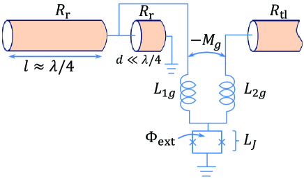
Figure 16: Schematic of the tunable coupler of Refs. Yin13 ; Wen14 between the $\lambda/4$ microwave resonator (at the left) and the transmission line (at the right). A voltage taken at the distance $d$ from the resonator end is applied to a transformer with a negative mutual inductance $-M_{g}$ and a SQUID providing positive Josephson inductance $L_{J}$. External flux $\Phi_{\rm ext}$ controls $L_{J}$, thus controlling the effective mutual inductance $M=-M_{g}+L_{J}$. The wave impedances of the lines are $R_{\rm r}$ and $R_{\rm tl}$.

The schematic of the tunable coupler is shown in Fig. 16. A quarter-wavelength ($\lambda/4$) microwave resonator is divided into two unequal parts, and the voltage signal for the coupler is taken at the distance $d$ ($d\ll\lambda/4$) from the end, which is shorted to the ground, while the other end is terminated with a break so that the total length is $l+d\approx\lambda/4$. The coupler consists of a transformer with geometrical inductances $L_{1g}$ and $L_{2g}$ and negative mutual inductance $-M_{g}$, which is in series with a dc SQUID, providing a positive Josephson inductance $L_{J}$. This inductance is controlled by an external magnetic flux $\Phi_{\rm ext}$, $L_{J}=\Phi_{0}/[2\pi\sqrt{I_{c1}^{2}+I_{c2}^{2}+2I_{c1}I_{c2}\cos(2\pi\Phi_{\rm ext}/\Phi_{0})}]$, where $\Phi_{0}=h/2e$ is the magnetic flux quantum and $I_{c1}$, $I_{c2}$ are the critical currents of two Josephson junctions, forming the SQUID. Thus the external flux controls the total mutual inductance $M=-M_{g}+L_{J}$, which determines the coupling between the resonator and transmission line; in particular, there is no coupling when $M=0$. Note that the wave impedance $R_{\rm r}$ of the resonator may be different from the impedance $R_{\rm tl}$ of the transmission line.

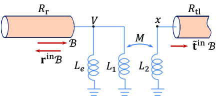
Figure 17: The simplified schematic of Fig. 16, with the $d$-long piece of the resonator replaced by inductance $L_{e}$, and the transformer in series with SQUID replaced by an effective transformer with mutual inductance $M$. An incident wave with voltage amplitude $\mathcal{B}$ creates voltages $V$ and $x$ across the inductors $L_{1}$ and $L_{2}$. The wave is reflected as $\textbf{r}^{\rm in}\mathcal{B}$ and transmitted as $\tilde{\bf t}^{\rm in}\mathcal{B}$ (the superscript “in” indicates the wave coming from inside the resonator and the tilde sign indicates the actual transmission amplitude, as opposed to the effective amplitude t). In our case ${\textbf{r}}^{\rm in}\approx-1$ and $|\tilde{\bf t}^{\rm in}|\ll 1$.

For the analysis let us first reduce the schematic of Fig. 16 to the schematic of Fig. 17 by replacing the $d$-long part of the resonator with an effective inductance $L_{e}$ and also replacing the transformer and SQUID with an effective transformer with inductances $L_{1}$, $L_{2}$, and mutual inductance $M$,

$$L_{1}=L_{1g}+L_{J},\,\,\,L_{2}=L_{2g}+L_{J},\,\,\,M=-M_{g}+L_{J}.$$ (68)

We emphasize that $M$ can be both positive and negative, so the coupling changes sign when $M$ crosses zero (the coupler is OFF when $M=0$). Note that by varying $M$ we also slightly change $L_{1}$ and $L_{2}$,

$$L_{1}=L_{1g}+M_{g}+M,~{}~{}L_{2}=L_{2g}+M_{g}+M.$$ (69)

It is easy to calculate the effective inductance $L_{e}$. If there is no coupler ($L_{1}=\infty$) and a voltage wave $\mathcal{B}e^{i\omega t}$ comes from the resonator side (from the left in Fig. 16), then it is reflected as $-\mathcal{B}e^{i\omega t}$, and the voltage at a distance $d$ is then $V=\mathcal{B}e^{i\omega t}[\exp(i\omega d/v)-\exp(-i\omega d/v)]=2i\mathcal{B}e^{i\omega t}\sin(\omega d/v)$, where $v$ is the speed of light in the resonator. The current (to the right) at this point is $I=(\mathcal{B}/R_{\rm r})e^{i\omega t}[\exp(i\omega d/v)+\exp(-i\omega d/v)]=2(\mathcal{B}/R_{\rm r})\cos(\omega d/v)$. Therefore, the wave impedance is $Z=V/I=iR_{\rm r}\tan(\omega d/v)$, which is the same, $Z=i\omega L_{e}$, as for an inductance

$$L_{e}=\frac{R_{\rm r}}{\omega}\tan\frac{\omega d}{v}=\frac{R_{\rm r}}{\omega}\tan\frac{2\pi d}{\lambda}.$$ (70)

Next, let us calculate the transmission and reflection amplitudes $\tilde{\bf t}^{\rm in}$ and ${\textbf{r}}^{\rm in}$ for the effective circuit shown in Fig. 17. (Here the superscript “in” reminds us that the wave is incident from inside of the resonator, and the tilde sign in $\tilde{\bf t}^{\rm in}$ means that we consider the actual transmission amplitude, which is different from the effective amplitude t). Assume that a voltage wave with amplitude $\mathcal{B}$ is incident onto the coupler from the resonator (we omit the exponential factor $e^{i\omega t}$). The wave is reflected as $\textbf{r}^{\rm in}\mathcal{B}$ and transmitted as $\tilde{\bf t}^{\rm in}\mathcal{B}$. For a weak coupling, which we consider in this paper, $\textbf{r}^{\rm in}\approx-1$ and $|\tilde{\bf t}^{\rm in}|\ll 1$. The voltage across $L_{1}$ is $V=(1+{\textbf{r}}^{\rm in})\mathcal{B}$, while the voltage across $L_{2}$ is denoted by $x$. The current flowing into $L_{1}$ is $I_{1}=(1-{\textbf{r}}^{\rm in})\mathcal{B}/R_{\rm r}-V/(i\omega L_{e})$, while the current flowing (down) into $L_{2}$ is $I_{2}=-x/R_{\rm tl}$. Using the currents $I_{1}$ and $I_{2}$, we write transformer equations for voltages $x$ and $V$ as

$$x=i\omega M\left[\frac{(1-{\textbf{r}}^{\rm in})\mathcal{B}}{R_{\rm r}}-\frac{(1+{\textbf{r}})^{\rm in}\mathcal{B}}{i\omega L_{e}}\right]-i\omega L_{2}\frac{x}{R_{\rm tl}},\,\,\,\,\qquad$$ (71)

$$(1+{\textbf{r}}^{\rm in})\mathcal{B}=i\omega L_{1}\left[\frac{(1-{\textbf{r}}^{\rm in})\mathcal{B}}{R_{\rm r}}-\frac{(1+{\textbf{r}}^{\rm in})\mathcal{B}}{i\omega L_{e}}\right]$$

$$\hskip 54.06006pt-i\omega M\frac{x}{R_{\rm tl}}.\,\,\qquad$$ (72)

From these two equations we can find the reflection amplitude ${\textbf{r}}^{\rm in}$ and the transmission amplitude $\tilde{\bf t}^{\rm in}=x/\mathcal{B}$ (note that $|\tilde{\bf t}^{\rm in}|^{2}R_{\rm r}/R_{\rm tl}+|{\textbf{r}}^{\rm in}|^{2}=1$):

$${\textbf{r}}^{\rm in}=-\frac{1-b}{1+b},$$ (73)

$$\tilde{\bf t}^{\rm in}=i\frac{2\omega M}{1+b}\left(\frac{1}{R_{\rm r}}+\frac{ib}{\omega L_{e}}\right)\frac{1}{1+i\omega L_{2}/R_{\rm tl}},$$ (74)

where

$$b=\frac{\displaystyle\frac{i\omega L_{1}}{R_{\rm r}}+\frac{\omega^{2}M^{2}}{R_{\rm r}R_{\rm tl}(1+i\omega L_{2}/R_{\rm tl})}}{\displaystyle 1+\frac{L_{1}}{L_{e}}-\frac{i\omega M^{2}}{R_{\rm tl}L_{e}(1+i\omega L_{2}/R_{\rm tl})}}$$ (75)

$$\hskip 8.5359pt=\frac{i\omega L_{1}/R_{\rm r}}{\displaystyle\frac{L_{1}}{L_{e}}+\left[1-\frac{i\omega M^{2}}{R_{\rm tl}L_{1}(1+i\omega L_{2}/R_{\rm tl})}\right]^{-1}}.\qquad$$ (76)

Note that the transmission and reflection amplitudes for the wave incident from outside of the resonator are

$$\tilde{\bf t}^{\rm out}=\frac{R_{\rm r}}{R_{\rm tl}}\,\tilde{\bf t}^{\rm in},\,\,\,{\textbf{r}}^{\rm out}=-\frac{\tilde{\bf t}^{\rm in}}{(\tilde{\bf t}^{\rm in})^{*}}\,{\textbf{r}}^{\rm in}.$$ (77)

Since the transmission amplitude depends on the direction, it is convenient to introduce the effective amplitude t, which does not depend on the direction,

$${\textbf{t}}=\sqrt{\frac{R_{\rm r}}{R_{\rm tl}}}\,\tilde{\bf t}^{\rm in}=\sqrt{\frac{R_{\rm tl}}{R_{\rm r}}}\,\tilde{\bf t}^{\rm out},\,\,\,|{\textbf{t}}|^{2}+|{\textbf{r}}^{\rm in(out)}|^{2}=1.$$ (78)

Equations (73)–(76) and (78) give us t and r in the rotating frame $e^{i\omega t}$. For the rotating frame $e^{-i\omega t}$ we need to conjugate t and r (and $b$), thus obtaining Eqs. (48)–(50) in the main text.

For an estimate let us use the following parameters (similar to the parameters of Ref. Yin13 ): $R_{\rm r}=80\,\Omega$, $R_{\rm tl}=50\,\Omega$, $L_{1g}=L_{2g}=480$ pH, $M_{g}=140$ pH, $\omega/2\pi=6$ GHz, and $L_{e}=180$ pH (corresponding to $d/\lambda=0.013$). Then Eqs. (73)–(76) and (78) for small $M$ give $b\approx 0.066i$, ${\textbf{r}}^{\rm in}\approx-e^{-0.13i}$, and ${\bf t}\approx 0.034ie^{-0.5i}M/M_{g}$. The resonator leakage time is then $\tau\approx(M_{g}/M)^{2}\times 72$ ns.

Note that in the case when $\omega M\ll R_{\rm tl}$, we can replace the denominator of Eq. (76) with $L_{1}/L_{e}+1$. Then

$$b\approx i\,\frac{\omega L_{e}/R_{\rm r}}{1+L_{e}/L_{1}},$$ (79)

and if $\omega L_{e}\ll R_{\rm r}$ (which means $d\ll\lambda/4$), then $|b|\ll 1$. In this case the reflection and effective transmission amplitudes (73) and (78) can be approximated (for the rotating frame $e^{i\omega t}$) as

$${\textbf{r}}^{\rm in}\approx-\exp\left[-\frac{2\omega L_{e}L_{1}}{R_{\rm r}(L_{1}+L_{e})}\,i\right]$$ (80)

$${\textbf{t}}\approx i\,\frac{2\omega L_{e}M}{\sqrt{R_{\rm r}R_{\rm tl}}\,(L_{1}+L_{e})}\,\frac{1}{1+i\omega L_{2}/R_{\rm tl}}.\qquad$$ (81)

The latter equation shows that in the first approximation the phase of t does not change with $M$, and for the case $\omega L_{2}\ll R_{\rm tl}$ the value of t is close to being purely imaginary. Note that Eq. (81) uses the approximation $1+b\approx 1$ in the denominator of the first factor in Eq. (74). Without this approximation (still using the above formula for $b$), the factor $L_{1}+L_{e}$ in the denominator of Eq. (81) should be replaced with a more accurate term $L_{1}+L_{e}+i\omega L_{1}L_{e}/R_{\rm r}$. As we checked numerically, this gives a much better approximation for small $M$ (mostly for the phase of t), but there is no significant improvement of accuracy for intermediate values of $M$, corresponding to $|\textbf{t}|\simeq 0.05$.

The resonator frequency $\omega_{\rm r}$ slightly changes when the mutual inductance $M$ is varied, because this slightly changes the phase of the reflection amplitude $\textbf{r}^{\rm in}$. The frequency change can be calculated as

$$\delta\omega_{\rm r}\approx 2\,\omega_{0}\,\frac{\delta(\arg{\textbf{r}}^{\rm in})}{2\pi},$$ (82)

where the factor of 2 comes from the assumption of a $\lambda/4$ resonator, and as $\omega_{0}$ we choose the resonator frequency at $M=0$. [Note the sign difference compared with Eq. (51) because of the different rotating frame.]

To estimate the frequency change $\Delta\omega_{\rm r}=\omega_{\rm r}(M)-\omega_{\rm r}(0)$ to first order, we can expand Eq. (76) to linear order in $M$ [which comes from changing $L_{1}$ in Eq. (79) – see Eq. (69)] and then use $\delta(\arg{\textbf{r}}^{\rm in})=-[2/(1+|b|^{2})]\,\delta|b|$, which follows from Eq. (73) for a positive-imaginary $b$. Thus we obtain

$$\Delta\omega_{\rm r}\approx-\frac{\omega_{0}}{\pi}\,\frac{2}{1+|b|^{2}}\,\frac{\omega_{0}L_{e}^{2}}{R_{\rm r}(L_{1}+L_{e})^{2}}\,M,$$ (83)

where $b$ is given by Eq. (79), and $L_{1}$ should be evaluated at $M=0$. Since t is also proportional to $M$ in the first order [see Eq. (74)], the ratio $\Delta\omega_{r}/|\textbf{t}|$ is approximately constant,

$$\frac{\Delta\omega_{\rm r}}{|\textbf{t}|}\approx-\frac{\omega_{0}}{\pi}\,\frac{\sqrt{1+(\omega_{0}L_{2}/R_{\rm tl})^{2}}}{\sqrt{1+|b|^{2}}}\sqrt{\frac{R_{\rm tl}}{R_{\rm r}}}\,\frac{L_{e}}{L_{1}+L_{e}},$$ (84)

where $L_{1}$ and $L_{2}$ should be evaluated at $M=0$, and for typical experimental parameters $|b|^{2}$ can be neglected [we keep the very small terms with $|b|^{2}$ in Eqs. (83) and (84) to have exact formulas at $M\rightarrow 0$]. This formula describes the numerical dependence $\Delta\omega_{\rm r}(|\textbf{t}|)$ shown in Fig. 12 very well, giving an exact result at $|{\textbf{t}}|\rightarrow 0$ and a relative deviation of 3.2% at $|{\textbf{t}}|=0.1$. It is interesting that the dependences of $|\textbf{t}|$ and $\Delta\omega_{\rm r}$ on $M$ are both significantly nonlinear (see, e.g., the dashed line in Fig. 12); however, these nonlinearities partially compensate each other to produce a smaller nonlinearity in $\Delta\omega_{\rm r}(|\textbf{t}|)$.

While Eq. (83) gives only the linear component of the dependence $\Delta\omega_{\rm r}(M)$, a better approximation can be based on using Eq. (79) to find $b(M)-b(0)$ and then convert it into $\Delta\omega_{\rm r}$ via Eq. (82). In this way we obtain

$$\Delta\omega_{\rm r}\approx-\,\frac{2\omega_{0}^{2}L_{e}^{2}/(1+|b|^{2})}{\pi R_{\rm r}(L_{1g}+M_{g}+L_{e})(L_{1g}+M_{g}+L_{e}+M)}\,M,$$ (85)

in which the term $|b|^{2}$ can be neglected. This formula gives a nonlinear dependence $\Delta\omega_{\rm r}(M)$ due to the presence of $M$ in the denominator. We checked that this formula correctly describes about 80% of the numerical nonlinearity of the $\Delta\omega_{\rm r}(M)$ dependence for the parameters of Fig. 12. There is a similar dependence on $M$ in the denominator of Eq. (81) for $\textbf{t}(M)$ dependence, thus explaining why the two nonlinearities partially cancel each other to produce a much more linear dependence $\Delta\omega_{\rm r}(|\textbf{t}|)$ in Fig. 12.

References

- (1) H. J. Kimble, Nature 453, 1023 (2008).
- (2) D. P. DiVincenzo, Fortschr. Phys. 48, 771 (2000).
- (3) J. I. Cirac, P. Zoller, H. J. Kimble, and H. Mabuchi, Phys. Rev. Lett. 78, 3221 (1997).
- (4) S. L. Braunstein and H. J. Kimble, Phys. Rev. Lett. 80, 869 (1998).
- (5) A. Furusawa, J. L. Sørensen, S. L. Braunstein, C. A. Fuchs, H. J. Kimble, and E. S. Polzik, Science 282, 706 (1998).
- (6) S. Lloyd, M. S. Shahriar, J. H. Shapiro, and P. R. Hemmer, Phys. Rev. Lett. 87, 167903 (2001).
- (7) L. M. Duan, M. D. Lukin, J. I. Cirac, and P. Zoller, Nature (London) 414, 413 (2001).
- (8) M. D. Lukin, Rev. Mod. Phys. 75, 457 (2003).
- (9) C. W. Chou, H. de Riedmatten, D. Felinto, S. V. Polyakov, S. J. van Enk, and H. J. Kimble, Nature (London) 438, 828 (2005).
- (10) M. Razavi and J. H. Shapiro, Phys. Rev. A 73, 042303 (2006).
- (11) S. Ritter, C. Nölleke, C. Hahn, A. Reiserer, A. Neuzner, M. Uphoff, M. Mücke, E. Figueroa, J. Bochmann, and G. Rempe, Nature 484, 195 (2012).
- (12) A. Stute, B. Casabone, B. Brandstätter, K. Friebe, T. E. Northup, and R. Blatt, Nature Phon. 7, 219 (2013).
- (13) K. Jahne, B. Yurke, and U. Gavish, Phys. Rev. A 75, 010301(R)(2007)
- (14) A.N. Korotkov, Phys. Rev. B 84, 014510 (2011).
- (15) T. Hime, P. A. Reichardt, B. L. T. Plourde, T. L. Robertson, C. E. Wu, A. V. Ustinov, and J. Clarke, Science 314, 1427 (2006).
- (16) A. O. Niskanen, K. Harrabi, F. Yoshihara, Y. Nakamura, S. Lloyd, and J. S. Tsai, Science 316, 723 (2007).
- (17) M. S. Allman, F. Altomare, J. D. Whittaker, K. Cicak, D. Li, A. Sirois, J. Strong, J. D. Teufel, and R. W. Simmonds, Phys. Rev. Lett. 104, 177004 (2010).
- (18) R. C. Bialczak, M. Ansmann, M. Hofheinz, M. Lenander, E. Lucero, M. Neeley, A. D. O’Connell, D. Sank, H. Wang, M. Weides, J. Wenner, T. Yamamoto, A. N. Cleland, and J. M. Martinis, Phys. Rev. Lett. 106, 060501 (2011).
- (19) A. J. Hoffman, S. J. Srinivasan, J. M. Gambetta, and A. A. Houck, Phys. Rev. B 84, 184515 (2011).
- (20) Yi Yin, Y. Chen, D. Sank, P. J. J. O’Malley, T. C. White, R. Barends, J. Kelly, E. Lucero, M. Mariantoni, A. Megrant, C. Neill, A. Vainsencher, J. Wenner, A. N. Korotkov, A. N. Cleland, and J. M. Martinis, Phys. Rev. Lett. 110, 107001 (2013).
- (21) S. J. Srinivasan, N. M. Sundaresan, D. Sadri, Y. Liu, J. M. Gambetta, T. Yu, S. M. Girvin, and A. A. Houck, Phys. Rev. A 89, 033857 (2014).
- (22) J. Wenner, Y. Yin, Yu Chen, R. Barends, B. Chiaro, E. Jeffrey, J. Kelly, A. Megrant, J. Y. Mutus, C. Neill, P. J. J. O’Malley, P. Roushan, D. Sank, A. Vainsencher, T. C. White, A. N. Korotkov, A. N. Cleland, and J. M. Martinis, Phys. Rev. Lett. 112, 210501 (2014).
- (23) Yu Chen, C. Neill, P. Roushan, N. Leung, M. Fang, R. Barends, J. Kelly, B. Campbell, Z. Chen, B. Chiaro, A. Dunsworth, E. Jeffrey, A. Megrant, J. Y. Mutus, P. J. J. O’Malley, C. M. Quintana, D. Sank, A. Vainsencher, J. Wenner, T. C. White, Michael R. Geller, A. N. Cleland, and J. M. Martinis, Phys. Rev. Lett. 113, 220502(2014).
- (24) J. D. Whittaker, F. C. S. da Silva, M. S. Allman, F. Lecocq, K. Cicak, A. J. Sirois, J. D. Teufel, J. Aumentado, and R. W. Simmonds, Phys. Rev. B 90, 024513 (2014).
- (25) M. Pierre, I.-M. Svensson, S. R. Sathyamoorthy, G. Johansson, and P. Delsing, Appl. Phys. Lett. 104, 232604 (2014).
- (26) J. Clarke and F. K. Wilhelm, Nature 453, 1031 (2008).
- (27) J. M. Gambetta, A. A. Houck, and A. Blais, Phys. Rev. Lett. 106, 030502 (2011).
- (28) E. A. Sete, A. Galiautdinov, E. Mlinar, J. M. Martinis, and A.N. Korotkov, Phys. Rev. Lett. 110, 210501 (2013).
- (29) J. Q. You, Z. D. Wang, W. Zhang, and F. Nori, Sci. Rep. 4, 5535 (2014).
- (30) R. Barends, J. Kelly, A. Megrant, A. Veitia, D. Sank, E. Jeffrey, T. C. White, J. Mutus, A. G. Fowler, B. Campbell, Y. Chen, Z. Chen, B. Chiaro, A. Dunsworth, C. Neill, P. O’Malley, P. Roushan, A. Vainsencher, J. Wenner, A. N. Korotkov, A. N. Cleland, and J. M. Martinis, Nature 508, 500 (2014).
- (31) J. M. Chow, J. M. Gambetta, E. Magesan, D. W. Abraham, A. W. Cross, B. R. Johnson, N. A. Masluk, C. A. Ryan, J. A. Smolin, S. J. Srinivasan, J. Srikanth, and M. Steffen, Nature Commun. 5, 4015 (2014).
- (32) S. J. Weber, A. Chantasri, J. Dressel, A. N. Jordan, K. W. Murch, and I. Siddiqi, Nature 511 570 (2014).
- (33) L. Sun, A. Petrenko, Z. Leghtas, B. Vlastakis, G. Kirchmair, K. M. Sliwa, A. Narla, M. Hatridge, S. Shankar, J. Blumoff, L. Frunzio, M. Mirrahimi, M. H. Devoret, and R. J. Schoelkopf, Nature 511, 7510 (2014).
- (34) Z. R. Lin, K. Inomata, K. Koshino, W. D. Oliver, Y. Nakamura, J. S. Tsai, and T. Yamamoto, Nature Comm. 5, 4480 (2014).
- (35) M. Stern, G. Catelani, Y. Kubo, C. Grezes, A. Bienfait, D. Vion, D. Esteve, and P. Bertet, Phys. Rev. Lett. 113, 123601 (2014).
- (36) L. Steffen, Y. Salathe, M. Oppliger, P. Kurpiers, M. Baur, C. Lang, C. Eichler, G. Puebla-Hellmann, A. Fedorov, and A. Wallraff, Nature 500, 319 (2013).
- (37) S. Gustavsson, O. Zwier, J. Bylander, F. Yan, F. Yoshihara, Y. Nakamura, T. P. Orlando, and W. D. Oliver, Phys. Rev. Lett. 110, 040502 (2013).
- (38) D. Riste, M. Dukalski, C. A. Watson, G. de Lange, M. J. Tiggelman, Y. M. Blanter, K. W. Lehnert, R. N. Schouten, and L. DiCarlo, Nature 502, 350 (2013).
- (39) N. Roch, M. E. Schwartz, F. Motzoi, C. Macklin, R. Vijay, A. W. Eddins, A. N. Korotkov, K. B. Whaley, M. Sarovar, and I. Siddiqi, Phys. Rev. Lett. 112, 170501 (2014).
- (40) M. Pechal, L. Huthmacher, C. Eichler, S. Zeytinoglu, A. A. Abdumalikov, Jr., S. Berger, A. Wallraff, and S. Filipp, Phys. Rev. X 4, 041010 (2014).
- (41) S. Zeytinoglu, M. Pechal, S. Berger, A. A. Abdumalikov Jr., A. Wallraff, S. Filipp, arXiv:1502.03692.
- (42) M. Keller, B. Lange, K. Hayasaka, W. Lange, and H. Walther, Nature 431, 1075 (2004).
- (43) P. Kolchin, C. Belthangady, S. Du, G. Y. Yin, and S. E. Harris, Phys. Rev. Lett. 101, 103601 (2008).
- (44) A. G. Fowler, M. Mariantoni, J. M. Martinis, and A. N. Cleland, Phys. Rev. A 86, 032324 (2012).
- (45) D. F. Walls and G. J. Milburn, Quantum optics (Springer, Berlin, 2008)
- (46) C. Gerry and P. Knight, Introductory Quantum Optics, (Cambridge University Press, Cambridge, UK, 2006)
- (47) B. Yurke and J. S. Denker, Phys. Rev. A 29, 1419 (1984).
- (48) M. A. Nielsen, Phys. Lett. A 303, 249 (2002).
- (49) M. Horodecki, P. Horodecki, and R. Horodecki, Phys. Rev. A 60, 1888 (1999).
- (50) K. Keane and A. N. Korotkov, Phys. Rev. A 86, 012333 (2012).
- (51) M. Hofheinz, H. Wang, M. Ansmann, R. C. Bialczak1, E. Lucero, M. Neeley, A. D. O’Connell, D. Sank, J. Wenner, J. M. Martinis, and A. N. Cleland, Nature 459, 546 (2009); Suppl. Information, Sec. 4.1.2.
- (52) M. Göppl, A. Fragner, M. Baur, R. Bianchetti, S. Filipp, J. M. Fink, P. J. Leek, G. Puebla, L. Steffen, and A. Wallraff, J. Appl. Phys. 104, 113904 (2008).
- (53) M. A. Nielsen and I. L. Chuang, Quantum Computation and Quantum Information (Cambridge University Press, Cambridge, UK, 2000).