Adaptive Optimal PMU Placement Based on Empirical Observability Gramian

Abstract

In this paper, we compare four measures of the empirical observability gramian, including the determinant, the trace, the minimum eigenvalue, and the condition number, which can be used to quantify the observability of system states and to obtain the optimal PMU placement for power system dynamic state estimation. An adaptive optimal PMU placement method is proposed by automatically choosing proper measures as the objective function. It is shown that when the number of PMUs is small and thus the observability is very weak, the minimum eigenvalue and the condition number are better measures of the observability and are preferred to be chosen as the objective function. The effectiveness of the proposed method is validated by performing dynamic state estimation on an Northeast Power Coordinating Council (NPCC) 48-machine 140-bus system with the square-root unscented Kalman filter.

1 Introduction

Increasing integration of intermittent renewable energy and current effort of developing smart grid will make electric power systems more and more dynamic. However, the most widely studied power system static state estimation (SSE) (Schweppe-Wildes (1970); Abur (2004); Monticelli (2000); Irving (2008); He (2011); Qi (2012)) cannot capture the dynamics of power systems well due to its dependency on slow update rates of Supervisory Control and Data Acquisition (SCADA) systems.

By contrast, real-time dynamic state estimation (DSE) enabled by phasor measurement units (PMUs), which has high update rates and high global positioning system (GPS) synchronization accuracy, can provide accurate dynamic states of the system and thus will play a critical role in achieving real-time wide-area monitoring, protection, and control (Begovic (2005); Qi (2015b)). Until now DSE has been implemented by extended Kalman filter (Huang (2007); Ghahremani (2011)), unscented Kalman filter (Wang (2012); Singh (2014)), square-root unscented Kalman filter (Qi (2015a, c)), extended particle filter (Zhou (2013)), cubature Kalman filter(Qi (2016a)), and observers (Taha (2015); Qi (2016a)).

The well-known optimal PMU placement (OPP) problem was originally developed for SSE. It is mainly based on the topological observability criterion, which only specifies that the power system states should be uniquely estimated with the minimum number of PMUS but neglects important parameters such as transmission line admittances by only focusing on the binary connectivity graph (Baldwin (1993); Li (2013)). Under this framework, many approaches have been proposed, such as mixed integer programming (Xu (2004); Gou (2008)), binary search (Chakrabarti (2008a)), metaheuristics (Milosevic (2003); Aminifar (2009)), particle swarm optimization (Chakrabarti (2008b)), and eigenvalue-eigenvector based approaches (Almutairi (2009); Korba (2003)). An information-theoretic criterion is also proposed to generate highly informative PMU configurations (Li (2013)).

However, not much research has been done on OPP for DSE. In (Kamwa (2002)) numerical PMU configuration algorithms are proposed to maximize the overall sensor response while minimizing the correlation among sensor outputs based on the system response under many contingencies. In (Sun (2011)) an OPP strategy is proposed to ensure a satisfactory state tracking performance but it depends on a specific Kalman filter. In (Qi (2015c)) the empirical observability gramian (Lall (1999, 2002); Hahn (2002); Singh (2006)) is applied to quantify the degree of observability of the system states and OPP is achieved by maximizing the determinant of the empirical observability gramian. Compared with (Kamwa (2002)) and (Sun (2011)), (Qi (2015c)) has a quantitative measure of observability, which makes it possible to optimize PMU locations from the point view of the observability of nonlinear systems. Besides, it only needs to deal with the system under typical power flow conditions and also does not depend on the specific realization of any Kalman filter.

As in (Qi (2015c)), there are various measures of the empirical observability gramian that can be used to quantify the observability of the system state. In this paper, we compare these measures and further propose an adaptive OPP method for power system dynamic state estimation by automatically choosing proper measures as the objective function to guarantee best observability.

The remainder of this paper is organized as follows. Section 2 briefly introduces power system dynamic state estimation. Section 3 discusses the definition and implementation of empirical observability gramian. Section 4 introduces the OPP method based on the empirical observability gramian and proposes an adaptive OPP method by making full use of different measures. The results are presented in Section 5 in order to test and validate the proposed method. Finally the conclusion is drawn in Section 6.

2 Power System Dynamic State Estimation

Different from SSE, DSE estimates the dynamic states (internal states of generators), rather than the static states (voltage magnitude and phase angles of buses). In order to perform DSE, the nonlinear dynamics and the outputs of a power system is described in the following form:

$$~{}\left\{\begin{array}[]{ll}\dot{\boldsymbol{x}}=\boldsymbol{f}(\boldsymbol{x},\boldsymbol{u})\\ \boldsymbol{y}=\boldsymbol{h}(\boldsymbol{x},\boldsymbol{u})\end{array}\right.$$ (1)

where $\boldsymbol{f}(\cdot)$ and $\boldsymbol{h}(\cdot)$ are the state transition and output functions, $\boldsymbol{x}\in\mathbb{R}^{n}$ is the state vector, $\boldsymbol{u}\in\mathbb{R}^{v}$ is the input vector, and $\boldsymbol{y}\in\mathbb{R}^{p}$ is the output vector.

We consider two types of generator models, the fourth-order transient model and second-order classical model. For generator with transient model, the fast sub-transient dynamics and saturation effects are ignored and the generator is described by fourth-order differential equations:

$$~{}\left\{\begin{array}[]{ll}\dot{\delta_{i}}=\omega_{i}-\omega_{0}\\ \dot{\omega}_{i}=\frac{\omega_{0}}{2H_{i}}\Big{(}T_{mi}-T_{ei}-\frac{K_{Di}}{\omega_{0}}(\omega_{i}-\omega_{0})\Big{)}\\ \dot{e}^{\prime}_{qi}=\frac{1}{T^{\prime}_{d0i}}\Big{(}E_{fdi}-e^{\prime}_{qi}-(x_{di}-x^{\prime}_{di})\,i_{di}\Big{)}\\ \dot{e}^{\prime}_{di}=\frac{1}{T^{\prime}_{q0i}}\Big{(}-e^{\prime}_{di}+(x_{qi}-x^{\prime}_{qi})\,i_{qi}\Big{)}\end{array}\right.$$ (2)

where $i$ is the generator serial number, $\delta_{i}$ is the rotor angle, $\omega_{i}$ is the rotor speed in rad/s, and $e^{\prime}_{qi}$ and $e^{\prime}_{di}$ are the transient voltage along $q$ and $d$ axes; $i_{qi}$ and $i_{di}$ are stator currents at $q$ and $d$ axes; $T_{mi}$ is the mechanical torque, $T_{ei}$ is the electric air-gap torque, and $E_{fdi}$ is the internal field voltage; $\omega_{0}$ is the rated value of angular frequency, $H_{i}$ is the inertia constant, and $K_{Di}$ is the damping factor; $T^{\prime}_{q0i}$ and $T^{\prime}_{d0i}$ are the open-circuit time constants for $q$ and $d$ axes; $x_{qi}$ and $x_{di}$ are the synchronous reactance and $x^{\prime}_{qi}$ and $x^{\prime}_{di}$ are the transient reactance at the $q$ and $d$ axes.

Generators with classical model are described by the first two equations of (2) and $e^{\prime}_{qi}$ and $e^{\prime}_{di}$ are kept unchanged.

$T_{mi}$ and $E_{fdi}$ are considered as inputs and are assumed to be constant and known. Let $\mathcal{G}_{P}$ denote the set of generators where PMUs are installed. For generator $i\in\mathcal{G}_{P}$, the terminal voltage phaosr $E_{ti}=e_{Ri}+je_{Ii}$ and the terminal current phasor $I_{ti}=i_{Ri}+ji_{Ii}$ can be measured, and are used as the outputs.

The dynamic model (2) can be rewritten in a general state space form in (1) and the state vector $\boldsymbol{x}$, input vector $\boldsymbol{u}$, and output vector $\boldsymbol{y}$ can be written as

$$\boldsymbol{x} =\begin{bmatrix}\boldsymbol{\delta}^{\top}\quad\boldsymbol{\omega}^{\top}\quad\boldsymbol{e^{\prime}_{q}}^{\top}\quad\boldsymbol{e^{\prime}_{d}}^{\top}\end{bmatrix}^{\top}$$ (3)

$$\boldsymbol{u} =\begin{bmatrix}\boldsymbol{T_{m}}^{\top}\quad\boldsymbol{E_{fd}}^{\top}\end{bmatrix}^{\top}$$ (4)

$$\boldsymbol{y} =\begin{bmatrix}\boldsymbol{e_{R}}^{\top}\quad\boldsymbol{e_{I}}^{\top}\quad\boldsymbol{i_{R}}^{\top}\quad\boldsymbol{i_{I}}^{\top}\end{bmatrix}^{\top}.$$ (5)

The $i_{qi}$, $i_{di}$, and $T_{ei}$ in (2) are actually functions of $\boldsymbol{x}$:

$$\it\Psi_{Ri} =e^{\prime}_{di}\sin\delta_{i}+e^{\prime}_{qi}\cos\delta_{i}$$

$$\it\Psi_{Ii} =e^{\prime}_{qi}\sin\delta_{i}-e^{\prime}_{di}\cos\delta_{i}$$

$$I_{ti} =\overline{\boldsymbol{Y}}_{i}(\boldsymbol{\it\Psi}_{R}+j\boldsymbol{\it\Psi}_{I})$$

$$i_{Ri} =\operatorname{Re}(I_{ti})$$

$$i_{Ii} =\operatorname{Im}(I_{ti})$$

$$i_{qi} =\frac{S_{B}}{S_{Ni}}(i_{Ii}\sin\delta_{i}+i_{Ri}\cos\delta_{i})$$

$$i_{di} =\frac{S_{B}}{S_{Ni}}(i_{Ri}\sin\delta_{i}-i_{Ii}\cos\delta_{i})$$

$$e_{qi} =e^{\prime}_{qi}-x^{\prime}_{di}i_{di}$$

$$e_{di} =e^{\prime}_{di}+x^{\prime}_{qi}i_{qi}$$

$$P_{ei} =e_{qi}i_{qi}+e_{di}i_{di}$$

$$T_{ei} =\frac{S_{B}}{S_{Ni}}P_{ei}$$

where $\it\Psi_{i}=\Psi_{Ri}+j\Psi_{Ii}$ is the voltage source, $\boldsymbol{\it\Psi}_{R}$ and $\boldsymbol{\it\Psi}_{I}$ are column vectors of all generators’ $\it\Psi_{Ri}$ and $\it\Psi_{Ii}$, $e_{qi}$ and $e_{di}$ are the terminal voltage at $q$ and $d$ axes, and $\overline{\boldsymbol{Y}}_{i}$ is the $i$th row of the admittance matrix of the reduced network $\boldsymbol{\overline{Y}}$ whose elements are constant if the difference between $x^{\prime}_{d}$ and $x^{\prime}_{q}$ is ignored (Wang (2015)), $P_{ei}$ is the electrical active output power, and $S_{B}$ and $S_{Ni}$ are the system base MVA and the base MVA for generator $i$, respectively.

The outputs $i_{R}$ and $i_{I}$ have been written as functions of $\boldsymbol{x}$. Similarly, the outputs $e_{Ri}$ and $e_{Ii}$ can also be written as function of $\boldsymbol{x}$:

$$e_{Ri} =e_{di}\sin\delta_{i}+e_{qi}\cos\delta_{i}$$

$$e_{Ii} =e_{qi}\sin\delta_{i}-e_{di}\cos\delta_{i}.$$

The continuous model in (1) can be discretized as

$$~{}\left\{\begin{array}[]{ll}\boldsymbol{x}_{k}=\boldsymbol{f}_{d}(\boldsymbol{x}_{k-1},\boldsymbol{u}_{k-1})\\ \boldsymbol{y}_{k}=\boldsymbol{h}(\boldsymbol{x}_{k},\boldsymbol{u}_{k})\end{array}\right.$$ (6)

where the state transition functions $\boldsymbol{f}_{d}$ can be obtained by the modified Euler method as

$$\tilde{\boldsymbol{x}}_{k} =\boldsymbol{x}_{k-1}+\boldsymbol{f}(\boldsymbol{x}_{k-1},\boldsymbol{u}_{k-1})\Delta t$$ (7)

$$\tilde{\boldsymbol{f}} =\frac{\boldsymbol{f}(\tilde{\boldsymbol{x}}_{k},\boldsymbol{u}_{k})+\boldsymbol{f}(\boldsymbol{x}_{k-1},\boldsymbol{u}_{k-1})}{2}$$ (8)

$$\boldsymbol{x}_{k} =\boldsymbol{x}_{k-1}+\tilde{\boldsymbol{f}}\Delta t.$$ (9)

3 Empirical Observability Gramian

Empirical observability gramian (Lall (1999, 2002); Hahn (2002); Singh (2006)) provide a computable tool for empirical analysis of the state-output behavior of nonlinear systems, which can be used to quantify the observability of the system state under some specific sensor placement.

The following sets are defined for empirical observability gramian:

$$T^{n}=\{\boldsymbol{T}_{1},\cdots,\boldsymbol{T}_{r};\;\;\;\boldsymbol{T}_{l}\in\mathbb{R}^{n\times n},\;\boldsymbol{T}_{l}^{\top}\boldsymbol{T}_{l}=\boldsymbol{I}_{n},\;l=1,\ldots,r\}$$

$$M=\{c_{1},\cdots,c_{s};\;\;\;\;c_{m}\in\mathbb{R},\;c_{m}>0,\;m=1,\ldots,s\}$$

$$E^{n}=\{\boldsymbol{e}_{1},\cdots,\boldsymbol{e}_{n};\;\;\;\textrm{standard unit vectors in}\;\mathbb{R}^{n}\}$$

where $T^{n}$ defines initial state perturbation directions, $r$ is the number of matrices for perturbation directions, $\boldsymbol{I}_{n}$ is an $n\times n$ identity matrix; $M$ defines perturbation sizes and $s$ is the number of different perturbation sizes for each direction, and $E^{n}$ defines the state to be perturbed and $n$ is the number of states.

For the nonlinear system described by (1), the empirical observability gramian can be defined as (Lall (1999))

$$\boldsymbol{W}_{o}^{con}=\sum_{l=1}^{r}\sum_{m=1}^{s}\frac{1}{rsc_{m}^{2}}\int_{0}^{\infty}\boldsymbol{T}_{l}\boldsymbol{\Psi}^{lm}(t)\boldsymbol{T}_{l}^{\top}dt$$ (10)

where $\boldsymbol{\Psi}^{lm}(t)\in\mathbb{R}^{n\times n}$ is given by $\boldsymbol{\Psi}_{ij}^{lm}(t)=(\boldsymbol{y}^{ilm}(t)-\boldsymbol{y}^{ilm,0})^{\top}(\boldsymbol{y}^{jlm}(t)-\boldsymbol{y}^{jlm,0})$, $\boldsymbol{y}^{ilm}(t)$ is the output of the nonlinear system corresponding to the initial condition $\boldsymbol{x}(0)=c_{m}\boldsymbol{T}_{l}\boldsymbol{e}_{i}+\boldsymbol{x}_{0}$, and $\boldsymbol{y}^{ilm,0}$ refers to the output measurement corresponding to the unperturbed initial state $\boldsymbol{x}_{0}$, which is usually chosen as the steady state under typical power flow conditions.

The discrete form of empirical observability gramian can be defined as (Hahn (2002))

$$\boldsymbol{W}_{o}=\sum_{l=1}^{r}\sum_{m=1}^{s}\frac{1}{rsc_{m}^{2}}\sum_{k=0}^{K}\boldsymbol{T}_{l}\boldsymbol{\Psi}^{lm}_{k}\boldsymbol{T}_{l}^{\top}\Delta t_{k}$$ (11)

where $\boldsymbol{\Psi}^{lm}_{k}\in\mathbb{R}^{n\times n}$ is given by ${\boldsymbol{\Psi}^{lm}_{k}}_{ij}=(\boldsymbol{y}^{ilm}_{k}-\boldsymbol{y}^{ilm,0})^{\top}(\boldsymbol{y}^{jlm}_{k}-\boldsymbol{y}^{jlm,0})$, $\boldsymbol{y}^{ilm}_{k}$ is the output at time step $k$ corresponding to initial condition $\boldsymbol{x}(0)=c_{m}\boldsymbol{T}_{l}\boldsymbol{e}_{i}+\boldsymbol{x}_{0}$, $\boldsymbol{y}^{ilm,0}$ is the output for unperturbed initial state $\boldsymbol{x}_{0}$, $K$ is the number of points, and $\Delta t_{k}$ is the time interval.

4 Adaptive Optimal PMU Placement

Based on the empirical observability gramian in (11), the OPP for dynamic state estimation can be formulated as

$$\max\limits_{\boldsymbol{z}}F\big{(}\,\boldsymbol{W}_{o}(\boldsymbol{z})\big{)}$$

s.t. $$\;\;\;\sum_{i=1}^{g}z_{i}=\bar{g}$$

$$z_{i} \in\{0,1\},\;\;i=1,\ldots,g$$ (12)

where $F$ is a function (measure) of the gramian $\boldsymbol{W}_{o}$, $\boldsymbol{z}$ is the vector of binary control variables determining PMU placement, and $g$ and $\bar{g}$ are, respectively, the number of generators and PMUs.

It has been shown that the empirical observability gramian for a system with $p$ outputs is the summation of the empirical gramians computed for each of the $p$ outputs individually (Singh (2006); Qi (2015c)). Obviously, the empirical observability gramian calculated from placing $\bar{g}$ PMUs individually adds to be the identical gramian calculated from placing the $\bar{g}$ PMUs simultaneously. Therefore, the optimization problem (4) can be rewritten as

$$\max\limits_{\boldsymbol{z}}F\Big{(}\,\sum_{i=1}^{g}z_{i}\boldsymbol{W}_{o,i}(\boldsymbol{z})\Big{)}$$

s.t. $$\qquad\sum_{i=1}^{g}z_{i}=\bar{g}$$

$$\qquad z_{i}\in\{0,1\},\;\;i=1,\ldots,g$$ (13)

where $\boldsymbol{W}_{o,i}$ is the empirical observability gramian by only placing one PMU at generator $i$.

The objective function $F$ quantifies the observability of the system state and can be the determinant ($\det$) (Qi (2015c, 2016b)), the trace ($\operatorname{Tr}$) (Singh (2006)), the smallest eigenvalue ($\sigma_{\min}$) (Kang (2009a, b, 2012); Sun (2014); Krener (2009)), or the opposite of the condition number ($-\kappa$) (Krener (2009)). By solving (4) an OPP can be obtained for each $\bar{g}$ and each $F$.

Different measures of the observability gramian reflect various aspects of observability. The determinant and the trace measure the overall observability in all directions in noise space. However, the trace cannot tell the existence of a zero eigenvalue and an unobservable system may still have a large trace. The smallest eigenvalue defines the worst scenario of observability while the condition number emphasizes the numerical stability in state estimation.

Although the determinant is a good measure that reflects the overall observability in all directions in noise space, it can be too small to be able to indicate the degree of observability, especially when the number of PMUs is small, in which case the observability for some states can be very weak and the determinant of the empirical observability gramian (the product of all eigenvalues) can be very small. When this is the case, the smallest eigenvalue or the condition number are better measures for quantifying the observability.

Based on this, we propose an adaptive OPP method by making use of the advantages of different measures as:

$$\boldsymbol{z}^{*}(\bar{g})=\left\{\begin{array}[]{ll}\boldsymbol{z}_{\det}^{*}(\bar{g})&\textrm{if $\det\big{(}\boldsymbol{z}_{\det}^{*}(\bar{g})\big{)}\geq\epsilon$}\\ \boldsymbol{z}_{-\kappa}^{*}(\bar{g})&\textrm{if $\det\big{(}\boldsymbol{z}_{\det}^{*}(\bar{g})\big{)}<\epsilon$ and $R_{-\kappa}\geq R_{\sigma_{\min}}$}\\ \boldsymbol{z}_{\sigma_{\min}}^{*}(\bar{g})&\textrm{if $\det\big{(}\boldsymbol{z}_{\det}^{*}(\bar{g})\big{)}<\epsilon$ and $R_{-\kappa}<R_{\sigma_{\min}}$}\end{array}\right.$$

where $\boldsymbol{z}^{*}(\bar{g})$ is the adaptive OPP for placing $\bar{g}$ PMUs, $\boldsymbol{z}_{F}^{*}(\bar{g})$ is the optimal placement of $\bar{g}$ PMUs by using $F\in\{\det,\sigma_{\min},-\kappa\}$ as the objective function in (4), and

$$R_{-\kappa}=\frac{\kappa\big{(}\boldsymbol{z}_{\det}^{*}(\bar{g})\big{)}}{\kappa\big{(}\boldsymbol{z}_{-\kappa}^{*}(\bar{g})\big{)}}\;,$$ (14)

$$R_{\sigma_{\min}}=\frac{\sigma_{\min}\big{(}\boldsymbol{z}_{\sigma_{\min}}^{*}(\bar{g})\big{)}}{\sigma_{\min}\big{(}\boldsymbol{z}_{\det}^{*}(\bar{g})\big{)}}$$ (15)

are used to indicate the improvement of the condition number using $-\kappa$ objective function or the minimum eigenvalue using $\sigma_{\min}$ objective function compared with using $\det$ objective function, and we write $F\Big{(}\sum_{i=1}^{g}z_{F,i}^{*}\boldsymbol{W}_{o,i}\big{(}\boldsymbol{z}^{*}_{F}(\bar{g})\big{)}\Big{)}$ in short as $F\big{(}\boldsymbol{z}^{*}_{F}(\bar{g})\big{)}$, which denotes the function value of $F\in\{\det,\sigma_{\min},\kappa\}$ for $\sum_{i=1}^{g}z_{F,i}^{*}(\bar{g})\boldsymbol{W}_{o,i}\big{(}\boldsymbol{z}^{*}_{F}(\bar{g})\big{)}$. When the determinant is less than $\epsilon$, the observability is too weak and the determinant is too small to be a good measure of observability. In this paper $\epsilon$ is chosen as $1$.

In the proposed adaptive optimal PMU placement method, the optimization problem in (4) has to be solved for three times. Compared with the method in Qi (2015c), this will increase the computational burden. However, since the PMU placement problem is used for planning and is solved offline, the calculation time is not a concern.

5 Case Study

The proposed method is tested on the NPCC 48-machine 140-bus system (Chow (1992)), which represents the northeast region of the Eastern Interconnection system. Among the 48 generators, 27 of them have fourth-order transient model and the others have second-order classical model. The map of this system is shown in Fig. 1.

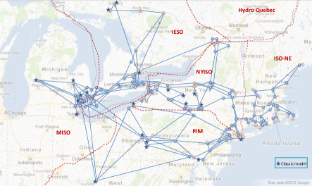
Figure 1: Map of the NPCC 48-machine 140-bus system. The stars indicates generators with classical model.

The empirical observability gramian calculation in (11) is implemented based on emgr (Empirical Gramian Framework) (Himpe (2013)) on time interval $[0,t_{f}]$. In this paper $t_{f}$ is chosen as 5 seconds.

The mixed-integer optimization problem in (4) is solved by NOMAD solver (Digabel (2011)), which is a derivative-free global mixed integer nonlinear programming solver and is called by the OPTI toolbox (Currie (2012)). NOMAD implements the Mesh Adaptive Direct Search (MADS) algorithm (Audet (2006)), a derivative-free direct search method with a rigorous convergence theory based on nonsmooth calculus (clarke (1990)), and aims for the best possible solution with a small number of evaluations.

DSE is performed by using square-root unscented Kalman filter (Merwe (2001); Qi (2015c, a)) for 50 times under OPP for different $F$ and random PMU placements to estimate the state trajectory on $[0,5s]$. For each case a three-phase fault is applied at the from bus of one of the 50 branches with highest line flows. Measurements are voltage phasors and current phasors from PMUs at generator terminal buses with a sampling rate of 60 frames/s. All the other settings are the same as (Qi (2015c)).

5.1 Comparing PMU Placements Using Different Measures of the Empirical Observability Gramian

In Fig. 2 we show the average error of rotor angles

$$\bar{e}_{\delta}=\sqrt{\frac{\sum\limits_{i=1}^{g}\sum\limits_{t=1}^{T_{s}}\big{(}\delta_{i,t}^{\textrm{est}}-\delta_{i,t}^{\textrm{true}}\big{)}^{2}}{g\,T_{s}}}$$ (16)

where $\delta_{i,t}^{\textrm{est}}$ and $\delta_{i,t}^{\textrm{true}}$ are the estimated and true rotor angles of the $i$th generator at time step $t$ and $T_{s}$ is the number of time steps.

Fig. 3 shows the average number of convergent angles, $\overline{N}_{\delta}$, for which the differences between the estimated and true values in the last one second are less than 2% of the absolute value of true values.

From these figures it is seen that:

1. Optimal placements are better than random placements in terms of guaranteeing better observability that can be indicated by smaller estimation error and greater number of convergent states.

2. $\operatorname{Tr}$ is not a good measure, mainly due to its being unable to tell the existence of a zero eigenvalue.

3. $\det$ is a good measure if the number of PMUs is not too small and the observability is not too weak; otherwise it has too small values to indicate observability.

4. $\sigma_{\min}$ and $-\kappa$ work better than $\det$ for small number of PMUs, in which case they have more reasonable values to indicate observability.

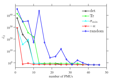
Figure 2: Average error for different PMU placements

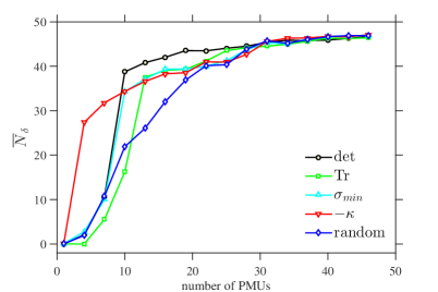
Figure 3: Number of convergent angles under different PMU placements.

5.2 Results for Adaptive Optimal PMU Placement

Fig. 4 illustrates the proposed method. When the number of PMUs $\bar{g}\geq 10$, $\det(\boldsymbol{z}_{\det}^{*})\geq 1$ ($\log\det(\boldsymbol{z}_{\det}^{*})\geq 0$) and thus the determinant is big enough to be used as objective function. When $\bar{g}<10$, $\sigma_{\min}$ or $-\kappa$ is considered. Since the improvement for condition number is higher ($R_{-\kappa}>R_{\sigma_{\min}}$), $-\kappa$ is chosen as the objective function.

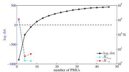
Figure 4: Illustration of the adaptive OPP method. The dash line denotes that the maximum determinant of the empirical observability gramian equals 1 (or equivalently the corresponding $\log\det$ equals 0).

In Fig. 5 we show the average numbers of convergent angles for adaptive OPP, which are much greater than those under random placements and are also better than those only using one measure as the objective function.

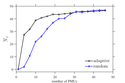
Figure 5: Number of convergent angles for adaptive OPP compared with random OPP.

6 Conclusion

In this paper, different measures of the empirical observability gramian that can quantify the degree of observability of a power system under a specific PMU configuration are compared and an adaptive optimal PMU placement method for dynamic state estimation is proposed by automatically choosing proper measures as the objective function to guarantee best observability. For systems with a relatively small number of PMUs, the observabiity measured by condition number and smallest eigenvalue are more reliable, i.e. the numerical stability and the worst case scenario have higher impact on the observability. On the other hand, if the number of PMUs is not too small, the determinant is a better overall measure of observability.

The proposed method is tested on the NPCC 48-machine 140-bus system by performing dynamic state estimation with square-root unscented Kalman filter. Compared with only using one measure to quantify observability, the proposed method can guarantee smaller estimation errors and larger number of convergent states.

The discussion on different measures of the empirical observability gramian should be valid for the empirical controllability gramian. The idea based on which the adaptive optimal PMU placement method is proposed should also work for other placement problems related to either observability or controllability, such as the dynamic var sources placement discussed in Qi (2016b).

References

- Abur (2004) A. Abur and A. Gómez Expósito (2004). Power System State Estimation: Theory and Implementation, CRC Press, 2004.
- Almutairi (2009) A. Almutairi and J. Milanovi (2009). Comparison of different methods for optimal placement of PMUs. Proc. IEEE Bucharest Power Tech Conf., Bucharest, Romania, pp. 1–6, Jun. 2009.
- Taha (2015) A. F. Taha, J. Qi, J. Wang, and J. H. Panchal (2016). Risk mitigation for dynamic state estimation against cyber attacks and unknown inputs. IEEE Trans. Smart Grid, in press.
- Krener (2009) A. J. Krener and K. Ide (2009). Measures of unobservability. IEEE Conf. Decision and Control, Shanghai, China, Dec. 2009.
- Singh (2014) A. K. Singh and B. C. Pal (2014). Decentralized dynamic state estimation in power systems using unscented transformation. IEEE Trans. Power Syst., vol. 29, no. 2, pp. 794–804, Mar. 2014.
- Singh (2006) A. K. Singh and J. Hahn (2002). Sensor location for stable nonlinear dynamic systems: multiple sensor case. Ind. Eng. Chem. Res., vol. 45, no. 10, pp. 3615–3623, 2006.
- Monticelli (2000) A. Monticelli (2000). “Electric power system state estimation,” Proc. IEEE, vol. 88, no. 2, pp. 262–282, Feb. 2000.
- Gou (2008) B. Gou (2008). Optimal placement of PMUs by integer linear programming. IEEE Trans. Power Syst., vol. 23, no. 3, pp. 1525–1526, Aug. 2008.
- Milosevic (2003) B. Milosevic and M. Begovic (2003). Nondominated sorting genetic algorithm for optimal phasor measurement placement. IEEE Trans. Power Syst., vol. 18, no. 1, pp. 69–75, Feb. 2003.
- Wang (2015) B. Wang and K. Sun (2015). Power System Differential-Algebraic Equations. arXiv:1512.05185, Dec. 2015.
- Xu (2004) B. Xu and A. Abur (2004). Observability analysis and measurement placement for systems with PMUs. in IEEE Power Syst. Conf. Expo., vol. 2, pp. 943–946, Oct. 2004.
- Audet (2006) C. Audet and J. E. Dennis Jr. (2006). Mesh adaptive direct search algorithms for constrained optimization. SIAM J. Optimiz., vol. 17, pp. 188–217, 2006.
- Himpe (2013) C. Himpe and M. Ohlberger (2013). A unified software framework for empirical gramians. J. Math., vol. 2013, pp. 1–6, 2013.
- Ghahremani (2011) E. Ghahremani and I. Kamwa (2011). Dynamic state estimation in power system by applying the extended Kalman filter with unknown inputs to phasor measurements. IEEE Trans. Power Syst., vol. 26, no. 4, pp. 2556–2566, Nov. 2011.
- Aminifar (2009) F. Aminifar, C. Lucas, A. Khodaei, and M. Fotuhi-Firuzabad (2009). Optimal placement of phasor measurement units using immunity genetic algorithm. IEEE Trans. Power Del., vol. 24, no. 3, pp. 1014–1020, Jul. 2009.
- Schweppe-Wildes (1970) F. C. Schweppe and J. Wildes (1970). Power system static-state estimation, Part I: exact model. IEEE Trans. Power App. Syst., vol. PAS-89, no. 1, pp. 120–125, Jan. 1970.
- clarke (1990) F. H. Clarke (1990). Optimization and nonsmooth analysis. Wiley, New York, NY. Reissued in 1990 by SIAM Publications, Philadelphia, PA.
- He (2011) G. He, S. Dong, J. Qi, and Y. Wang (2011). Robust state estimator based on maximum normal measurement rate. IEEE Trans. Power Syst., vol. 26, no. 4, pp. 2058–2065, Nov. 2011.
- Kamwa (2002) I. Kamwa and R. Grondin (2002). PMU configuration for system dynamic performance measurement in large multiarea power systems. IEEE Trans. Power Syst., vol. 17, no. 2, pp. 385–394, May 2002.
- Currie (2012) J. Currie and D. I. Wilson (2012). OPTI: lowering the barrier between open source optimizers and the industrial MATLAB user. Foundations of Computer-Aided Process Operations, Georgia, USA, 2012.
- Hahn (2002) J. Hahn and T. F. Edgar (2002). Balancing approach to minimal realization and model reduction of stable nonlinear systems. Ind. Eng. Chem. Res., vol. 41, no. 9, pp. 2204–-2212, 2002.
- Chow (1992) J. H. Chow and K. W. Cheung (1992) A toolbox for power system dynamics and control engineering education and research. IEEE Trans. Power Syst., vol. 7, no. 4, pp. 1559–1564, 1992.
- Qi (2016a) J. Qi, A. F. Taha, and J. Wang (2016a). Comparing Kalman filters and observers for dynamic state estimation with model uncertainty and malicious cyber attacks. arXiv preprint arXiv:1605.01030, 2016.
- Qi (2012) J. Qi, G. He, S. Mei, and F. Liu (2012). Power system set membership state estimation. in IEEE Power and Energy Society General Meeting, pp. 1–7, San Diego, CA USA, Jul. 2012.
- Qi (2015a) J. Qi, K. Sun, J. Wang, and H. Liu (2015a). Dynamic state estimation for multi-machine power system by unscented Kalman filter with enhanced numerical stability. arXiv preprint arXiv:1509.07394.
- Qi (2015b) J. Qi, K. Sun, and S. Mei (2015b). An interaction model for simulation and mitigation of cascading failures. IEEE Trans. Power Syst., vol. 30, no. 2, pp. 804–819, Mar. 2015.
- Qi (2015c) J. Qi, K. Sun, and W. Kang (2015c). Optimal PMU placement for power system dynamic state estimation by using empirical observability gramian. IEEE. Trans. Power Syst., vol. 30, no. 4, Jul. 2015.
- Qi (2016b) J. Qi, W. Huang, K. Sun, and W. Kang (2016b) Optimal placement of dynamic var sources by using empirical controllability covariance. IEEE. Trans. Power Syst., in press, 2016.
- Sun (2014) K. Sun, J. Qi, and W. Kang (2016). Power system observability and dynamic state estimation for stability monitoring using synchrophasor measurements. Control Engineering Practice, in press, 2016.
- Begovic (2005) M. Begovic, D. Novosel, D. Karlsson, C. Henville, and G. Michel (2005). Wide-area protection and emergency control. Proc. IEEE, vol. 93, no. 5, pp. 876–891, May 2005.
- Irving (2008) M. R. Irving (2008). Robust state estimation using mixed integer programming. IEEE Trans. Power Syst., vol. 23, no. 3, pp. 1519–1520, Aug. 2008.
- Zhou (2013) N. Zhou, D. Meng, and S. Lu (2013). Estimation of the dynamic states of synchronous machines using an extended particle filter. IEEE Trans. Power Syst., vol. 28, no. 4, pp. 4152–4161, Nov. 2013.
- Korba (2003) P. Korba, M. Larsson and C. Rehtanz (2003). Detection of Oscillations in Power Systems using Kalman Filtering Techniques. Proc. IEEE Conf. Control Applications, Istanbul, Turkey, pp. 183–188, Jun. 2003.
- Li (2013) Q. Li, T. Cui, Y. Weng, R. Negi, F. Franchetti, and M. Ilić (2013). An information-theoretic approach to PMU placement in electric power systems. IEEE Trans. Smart Grid, vol. 4, pp. 446–456, Mar. 2013.
- Merwe (2001) R. Merwe and E. Wan (2001). The square-root unscented Kalman filter for state and parameter-estimation. in Proc. IEEE Int. Conf. Acoust., Speech, and Signal Process., vol. 6, pp. 3461–3464, 2001.
- Chakrabarti (2008a) S. Chakrabarti and E. Kyriakides (2008a). Optimal placement of phasor measurement units for power system observability. IEEE Trans. Power Syst., vol. 23, no. 3, pp. 1433–1440, Aug. 2008.
- Chakrabarti (2008b) S. Chakrabarti, G. K. Venayagamoorthy and E. Kyriakides (2008b). PMU placement for power system observability using binary particle swarm optimization. Australasian Universities Power Engineering Conference, Brisbane, Australia, pp. 1–5, Dec. 2008.
- Lall (1999) S. Lall, J. E. Marsden, and S. Glavaški (1999). Empirical model reduction of controlled nonlinear systems. 14th IFAC World Congress, Beijing China, 1999.
- Lall (2002) S. Lall, J. E. Marsden, and S. Glavaški (2002). A subspace approach to balanced truncation for model reduction of nonlinear control systems. Int. J. Robust and Nonlinear Control, vol. 12, pp. 519–535, 2002.
- Digabel (2011) S. Le Digabel (2011). Algorithm 909: NOMAD: Nonlinear optimization with the MADS algorithm. ACM Trans. Mathematical Software, vol. 37, Feb. 2011.
- Wang (2012) S. Wang, W. Gao, and A. P. Meliopoulos (2012). An alternative method for power system dynamic state estimation based on unscented transform. IEEE Trans. Power Syst., vol. 27, no. 2, pp. 942–950, May 2012.
- Baldwin (1993) T. Baldwin, L. Mili, J. Boisen, M.B., and R. Adapa (1993). Power system observability with minimal phasor measurement placement. IEEE Trans. Power Syst., vol. 8, no. 2, pp. 707–715, May 1993.
- Kang (2009a) W. Kang and L. Xu (2009a). Computational analysis of control systems using dynamic optimization. arXiv:0906.0215v2.
- Kang (2009b) W. Kang and L. Xu (2009b) A quantitative measure of observability and controllability. 48th IEEE CDC, Shanghai, China.
- Kang (2012) W. Kang and L. Xu (2012) Optimal placement of mobile sensors for data assimilations. Tellus A, vol. 64, pp. 17133, 2012.
- Sun (2011) Y. Sun, P. Du, Z. Huang, K. Kalsi, R. Diao, K. K. Anderson, Y. Li, and B. Lee (2011). PMU placement for dynamic state tracking of power systems. North American Power Symposium, pp. 1–7, Aug. 2011.
- Huang (2007) Z. Huang, K. Schneider, and J. Nieplocha (2007). Feasibility studies of applying Kalman filter techniques to power system dynamic state estimation. Power Engr. Conf., pp. 376–382, Dec. 2007.