Division polynomials with Galois group $SU_{3}(3).2\!\cong\!G_{2}(2)$

Abstract.

We use a rigidity argument to prove the existence of two related degree twenty-eight covers of the projective plane with Galois group $SU_{3}(3).2\cong G_{2}(2)$. Constructing corresponding two-parameter polynomials directly from the defining group-theoretic data seems beyond feasablity. Instead we provide two independent constructions of these polynomials, one from $3$-division points on covers of the projective line studied by Deligne and Mostow, and one from $2$-division points of genus three curves studied by Shioda. We explain how one of the covers also arises as a $2$-division polynomial for a family of $G_{2}$ motives in the classification of Dettweiler and Reiter. We conclude by specializing our two covers to get interesting three-point covers and number fields which would be hard to construct directly.

1. Introduction

Suppose $Y$ is a variety over ${\mathbb{Q}}$ with bad reduction at a set $S$ of primes. For any prime $\ell$, there are associated number fields coming from the mod $\ell$ cohomology of the topological space $Y({\mathbb{C}})$. On the one hand, these number fields are interesting because their Galois groups tend to be Lie-type groups and their bad reduction is constrained to be within $S\cup\{\ell\}$. On the other hand, defining polynomials for these number fields are often beyond computational reach, even for quite simple $Y$ and very small $\ell$. In this paper, we work out some remarkable examples in this framework, with our computations of defining polynomials being ad hoc and just within the limits of feasibility.

1.1. Section-by-section overview

Section 2 provides background on the theoretical context, presenting it as a generalization of the familiar passage from an elliptic curve to one of its division polynomials. It then gives information on the Lie-type group which plays the central role for us, namely $SU_{3}(3).2\cong G_{2}(2)$. Finally, the section reviews an earlier construction of a one-parameter polynomial for this Galois group due to Malle and Matzat [12, p. 412].

Section 3 explains how a rigidity argument gives two canonical degree twenty-eight covers of surfaces defined over ${\mathbb{Q}}$, each with Galois group $SU_{3}(3).2\cong G_{2}(2)$. In our notation, these covers are

$$\pi_{1}:X_{1} \rightarrow U_{3,1,1}, \pi_{2}:X_{2} \rightarrow U_{3,2}.$$

The bases are respectively $U_{3,1,1}=M_{0,5}/S_{3}$ and $U_{3,2}=M_{0,5}/(S_{3}\times S_{2})$, these being moduli spaces of five partially distinguishable points in the projective line. We explain how the covers are related by a cubic correspondance deduced from an exceptional isomorphism $U_{2,1,1,1}\cong U_{2,1,2}$ first studied by Deligne and Mostow [5, §10]. Standard methods, as illustrated in [15], might let one construct the covers $\pi_{i}$ directly if certain curves had genus zero. However these methods are obstructed by the fact that these curves have positive genus.

Sections 4, 5, and 6 concern varietal sources for our covers. Section 4 starts with two different two-parameter families of covers of the projective line considered by Deligne and Mostow [4]. Via the group $SU_{3}(3).2$, these families of curves yield $\pi_{1}$ and $\pi_{2}$ from $3$-division points. We use the second family to compute a defining polynomial $F_{2}(a,b,x)$ for $\pi_{2}$, and then transfer this knowledge to also obtain a polynomial $F_{1}(p,q,x)$ for $\pi_{1}$. Section 5 starts with a large family of genus three curves studied by Shioda [17]. This family already has an explicit $2$-division polynomial $S(r_{1},r_{3},r_{4},r_{5},r_{6},r_{7},r_{9},z)$ with Galois group $Sp_{6}(2)$. We find appropriate loci in the parameter space where the Galois group drops to the subgroup $G_{2}(2)$, and thereby independently get alternative polynomials $S_{1}(p,q,z)$ and $S_{2}(a,b,z)$ for the two covers. Section 6 explains how $F_{1}(p,q,z)$ also arises as the $2$-division polynomial of a family of motives with motivic Galois group $G_{2}$ studied by Dettweiler and Reiter [6]. Sections 4, 5, and 6 each close with subsection explicitly relating $L$-polynomials modulo the relevant prime $\ell$ to our division polynomials.

Section 7 shifts the focus away from varietal sources and onto specializations of our explicit polynomials. Specializing to suitable lines, we get fourteen new degree twenty-eight three-point covers with Galois group $SU_{3}(3).2\cong G_{2}(2)$. These covers all have positive genus, and it would be difficult to construct them directly by the standard techniques of three-point covers.

Section 8 specializes to points, finding 376 different degree $28$ number fields with Galois group $SU_{3}(3).2\cong G_{2}(2)$ and discriminant of the form $2^{a}3^{b}$. Again it would be difficult to construct these fields by techniques within algebraic number theory itself. We show that a thorough analysis of ramification in these fields is possible, despite the relatively large degree, by presenting such an analysis of the field with the smallest discriminant.

1.2. Computer platforms.

The bulk of the calculations for this paper were carried out in Mathematica [19]. However most calculations with number fields were done in Pari [13] while most calculations with $L$-functions were done in Magma [2].

Many of the statements in this paper can only be confirmed with the assistance of a computer. To facilitate verification and further exploration on the reader’s part, a commented Mathematica file on the author’s homepage accompanies this paper. It contains some of the formulas and data presented here.

1.3. Relation to a similar paper.

The polynomials $F_{1}(p,q,x)$ and $F_{2}(a,b,x)$ are similar in nature to the polynomials $g_{27}(u,v,x)$ and $g_{28}(u,v,x)$ of [15] which have Galois groups $W(E_{6})$ and $W(E_{7})^{+}$ respectively. However [15] and this paper focus on different theoretical topics to avoid duplication. The discussion of monodromy and the universality of specialization sets in [15] applies after modification to the new base schemes $U_{3,1,1}$ and $U_{3,2}$ here. Similarly, our general discussion of division polynomials here could equally well be illustrated by $g_{27}(u,v,x)$ and $g_{28}(u,v,x)$ .

1.4. Acknowledgements

It is a pleasure to thank Zhiwei Yun for a conversation about $G_{2}$-rigidity from which this paper grew. It is equally a pleasure to thank Michael Dettweiler and Stefan Reiter for helping to make the direct connections to their work [6]. We are also grateful to the Simons Foundation for research support through grant #209472.

2. Background

This section provides some context for our later considerations.

2.1. Division Polynomials

Classical formulas [18, p. 200] let one pass directly from an elliptic curve $X:y^{2}=x^{3}+ax+b$ to division polynomials giving $x$-coordinates of their $n$-torsion points. Initializing via $f_{1}=1$ and $f_{2}=2$, these division polynomials $f_{n}$ for $n\geq 3$ are computable by recursion:

$$f_{3} = 3x^{4}+6ax^{2}+12bx-a^{2},$$

$$f_{4} = 4x^{6}+20ax^{4}+80bx^{3}-20a^{2}x^{2}-16abx-4a^{3}-32b^{2},$$

$$f_{2m} = f_{m}\left(f_{m+2}f_{m-1}^{2}-f_{m-2}f_{m+1}^{2}\right)/2,$$

$$f_{4m+1} = (x^{3}+ax+b)^{2}f_{2m+2}f_{2m}^{3}-f_{2m-1}f_{2m+1}^{3},$$

$$f_{4m+3} = f_{2m+3}f_{2m+1}^{3}-(x^{3}+ax+b)^{2}f_{2m}f_{2m+2}^{3}.$$

Special cases give interesting number fields. For example, at $(a,b)=(-1/3,19/108)$ the degree sixty polynomial $f_{11}\in{\mathbb{Q}}[x]$ has Galois group $GL_{2}(11)/\{\pm 1\}$ and field discriminant $-11^{109}$.

On an abstract level, there are interesting number fields from $n$-torsion points on any abelian variety over ${\mathbb{Q}}$. More generally, from any variety $Y$ over ${\mathbb{Q}}$ there are interesting field extensions from the natural action of $\mbox{Gal}(\overline{{\mathbb{Q}}}/{\mathbb{Q}})$ on the cohomology groups $H^{m}(Y({\mathbb{C}}),{\mathbb{Z}}/n{\mathbb{Z}})$. However for most pairs $(X,n)$, there is nothing remotely as explicit as the above recursion relations. In fact, there is presently no way at all to produce explicit division polynomials describing these fields.

2.2. The group $SU_{3}(3).2\cong G_{2}(2)$

The Atlas [3] provides a wealth of group-theoretic information about the group $SU_{3}(3).2\cong G_{2}(2)$. In particular, this group has the form $\Gamma.2$, where $\Gamma$ has order $6048=2^{5}3^{3}7$ and is the $12^{\rm th}$ smallest non-abelian simple group.

$$\begin{array}[]{| lr ll |}\hline\cr\vrule\lx@intercol\hfil\mbox{Classes in $\Gamma$}\hfil\lx@intercol\vrule\lx@intercol\\ C&|C|&\lambda_{28}&\lambda_{36}\\ \hline\cr 1A&1&1^{28}&1^{36}\\ 2A&63&2^{12}1^{4}&2^{12}1^{12}\\ 3A&56&3^{9}1&3^{12}\\ 3B&672&3^{9}1&3^{11}1^{3}\\ 4AB&2\cdot 63&4^{6}1^{4}&4^{6}2^{6}\\ 4C&378&4^{6}2^{2}&4^{6}2^{4}1^{4}\\ 6A&504&6^{4}31&6^{4}3^{4}\\ 7AB&2\cdot 864&7^{4}&7^{5}1\\ 8AB&2\cdot 756&8^{3}2^{1}1^{2}&8^{3}4^{3}\\ 12AB&2\cdot 504&12^{2}31&12^{2}6^{2}\\ \hline\cr\end{array}\;\;\;\;\;\;\;\;\;\;\;\;\begin{array}[]{|lrll|}\hline\cr\vrule\lx@intercol\hfil\mbox{Classes in $\Gamma.2-\Gamma$}\hfil\lx@intercol\vrule\lx@intercol\\ C&|C|&\lambda_{28}&\lambda_{36}\\ \hline\cr&&&\\ 2b&252&2^{12}1^{4}&2^{16}1^{4}\\ &&&\\ &&&\\ 4d&252&4^{6}1^{4}&4^{6}2^{6}\\ &&&\\ 6b&2016&6^{4}31&6^{5}3^{1}2^{1}1\\ &&&\\ 8c&1512&8^{3}4&8^{3}4^{2}21^{2}\\ 12cd&2\cdot 1008&12^{2}31&12^{2}6^{2}\\ \hline\cr\end{array}$$

Table 2.1. Information about conjugacy classes in $\Gamma.2$

Table 2.1 presents some of the information that is most important to us. The left half corresponds to the $14$ conjugacy classes in $\Gamma$. The six classes $1A$, $2A$, $3A$, $3B$, $4C$, and $6A$ are rational, while the remaining classes are conjugate in pairs over the quadratic fields ${\mathbb{Q}}(i)$, ${\mathbb{Q}}(\sqrt{-7})$, ${\mathbb{Q}}(i)$, and ${\mathbb{Q}}(i)$ respectively. When one considers the full group $\Gamma.2$, these pairs collapse and one has $16$ conjugacy classes, ten in $\Gamma$ and six in $\Gamma.2-\Gamma$, with $12c$ and $12d$ two classes conjugate over ${\mathbb{Q}}(\sqrt{-3})$.

Of particular importance to us is that $\Gamma.2$ embeds as a transitive subgroup of the alternating group $A_{28}$. The cycle partition $\lambda_{28}$ associated to a conjugacy class is given in Table 2.1. The group $\Gamma.2$ also embeds as a transitive subgroup of $A_{36}$ and the corresponding $\lambda_{36}$ are given. We use the degree $36$ embedding only occasionally. For example, it is useful for distinguishing $3A$ from $3B$ via cycle partitions. As a convention, if we do not refer explicitly to degree we are working with the degree twenty-eight embedding.

As just discussed, Table 2.1 has information about permutation representations of $\Gamma.2$. We are also interested in linear representations, and some group-theoretic information is contained in the small tables at the end of §4.3 (for characteristic 3), at the end of §5.5 (for characteristic 2), and in Figure 6.1 (for characteristic zero).

2.3. Rigidity and covers

Some fundamental aspects of our general context are as follows. Let $G$ be a finite centerless group and let $C=(C_{1},\dots,C_{z})$ be a list of conjugacy classes in $G$. Define

$$\overline{\Sigma}(C) = \{(g_{1},\dots,g_{z})\in C_{1}\times\cdots\times C_{z}:g_{1}\dots g_{z}=1\},$$

$${\Sigma}(C) = \{(g_{1},\dots,g_{z})\in\overline{\Sigma}(C):\langle g_{1},\dots,g_{z}\rangle=G\}.$$

The group $G$ acts on these sets by simultaneous conjugation and the action is free on ${\Sigma}(C)$. The mass of $C$ is $\overline{\mu}(C):=|\overline{\Sigma}(C_{1},\dots,C_{z})|/|G|$. A classical formula, presented in e.g. [12, Theorem 5.8], gives the mass as a sum over irreducible characters of $G$,

(2.1) $$\overline{\mu}(C)=\frac{|C_{1}|\cdots|C_{z}|}{|G|^{2}}\sum_{\chi}\frac{\chi(C_{1})\cdots\chi(C_{z})}{\chi(1)^{z-2}}.$$

We say that $C$ is rigid if $\mu(C):=|\Sigma(C)|/|G|=1$ and strictly rigid if moreover $\overline{\mu}(C)=1$.

Let $G\subseteq S_{n}$ now be a transitive permutation realization of $G$ such that the centralizer of $G$ in $S_{n}$ is trivial. Let $\tau_{1}$, …, $\tau_{z}$ be distinct points in the complex projective line, connected by suitable paths to a fixed basepoint. A tuple $(g_{1},\dots,g_{z})\in\Sigma(C)$ then determines a degree $n$ cover of the projective line with monodromy group $G$ and local monodromy transformation $g_{i}$ about the point $\tau_{i}$. The genus $g_{n}$ of the degree $n$ cover is calculated via the cycle partitions $\lambda_{i}\vdash n$ by the general formula

(2.2) $$|\lambda_{1}|+\dots+|\lambda_{z}|=(z-2)n+2-2g_{n}.$$

Here $|\lambda_{i}|$ indicates the number of parts of $\lambda_{i}$.

Let $M_{0,w}$ be the moduli space of $w$ labeled distinct points in the projective line. This is a very explicit space, as $\tau_{1}$, $\tau_{2}$, and $\tau_{3}$ can be uniquely normalized to $0$, $1$, and $\infty$ respectively. The group $S_{w}$ acts on $M_{0,w}$ by permuting the points. If $\nu=(\nu_{1},\dots,\nu_{r})$ sums to $w$ then we let $S_{\nu}=S_{\nu_{1}}\times\cdots\times S_{\nu_{r}}$ and put $U_{\nu}=M_{0,w}/S_{\nu}$.

When $C=(C_{1},\dots,C_{z})$ is rigid and the $\tau_{i}$ move in $M_{0,z}$, all the covers of the projective line fit together into a single cover of $M_{0,z+1}$. Moreover, under simple conditions as exemplified below, this cover is guaranteed to be defined over ${\mathbb{Q}}$. When $z=3$, the space $M_{0,3}$ is just a single point and $M_{0,4}$ identified with ${\mathbb{P}}^{1}-\{0,1,\infty\}$, with $\tau_{4}$ serving as coordinate. This case has been extensively treated in the literature. When $z\geq 4$ the situation is more complicated and a primary purpose of [15] and the present paper is to give interesting examples. When some adjacent $C_{i}$ coincide, the cover descends to a cover of the corresponding quotient $U_{\nu}$ of $M_{0,z+1}$.

2.4. The Malle-Matzat cover

Malle and Matzat computed the cover coming from the strictly rigid genus zero triple $(4d,\,2b,12AB)$ belonging to the group $\Gamma.2$. This Malle-Matzat cover is similar, but much simpler, than the covers $\pi_{1}$ and $\pi_{2}$ that we are about to consider. Accordingly we discuss it here as a model, and use it later as well for comparison.

Identifying the degree twenty-eight covering curve $X$ with ${\mathbb{P}}_{x}^{1}$, the cover ${\mathbb{P}}_{x}^{1}\rightarrow{\mathbb{P}}_{t}^{1}$ is then given by the explicit degree twenty-eight rational function $t=$

$$\frac{-\!\left(x^{6}-6x^{5}-435x^{4}-308x^{3}+15x^{2}+66x+19\right)^{\!4}\!\left(x^{4}+20x^{3}+114x^{2}+68x+13\right)}{2^{2}3^{9}\left(x^{2}+4x+1\right)^{12}(2x+1)}.$$

The partitions $\lambda_{1}=4^{6}1^{4}$ and $\lambda_{3}=12^{2}3\,1$ are visible as root multiplicities of the numerator and denominator respectively. Rewriting the equation as

(2.3) $$m(t,x)=0,$$

the partition $\lambda_{2}=2^{12}1^{4}$ likewise appears as the root multiplicities of $m(1,x)$.

The discriminant of the monic polynomial $m(t,x)$ is

(2.4) $$D_{m}(t)=2^{576}3^{630}t^{18}(t-1)^{12}.$$

It is a perfect square, in conformity with the fact that $\Gamma.2$ lies in the alternating group $A_{28}$. Thus $D_{m}(t)$ is not useful in seeing how the $.2$ enters Galois-theoretically. In fact, the order two quotient group corresponds to the extension of ${\mathbb{Q}}(t)$ generated by $\sqrt{t(1-t)}$.

The general theory of three-point covers says that $X\rightarrow{\mathbb{P}}_{t}$ has bad reduction within the primes dividing $|\Gamma.2|$, namely $2$, $3$, and $7$. A particularly interesting feature of $D_{m}(t)$ is that it reveals that in fact the Malle-Matzat cover has good reduction at $7$. In [14, §8], we explained how the Malle-Matzat polynomial is a division polynomial for a family of varieties with bad reduction only in $\{2,3\}$, and this connection explains the good reduction at $7$.

3. Rigid covers of $U_{3,1,1}$ and $U_{3,2}$

This section explains how general theory gives the existence of our two main covers $\pi_{1}:X_{1}\rightarrow U_{3,1,1}$ and $\pi_{2}:X_{2}\rightarrow U_{3,2}$ and the cubic relation between them.

3.1. Five strictly rigid quadruples

For a fixed number of ramifying points $z$ and a fixed ambient group $G$, the mass formula (2.1) lets one find all $C$ with $\overline{\mu}(C)=1$. From any explicit tuple $(g_{1},\dots,g_{z})\in\overline{\Sigma}(C)$, one gets $\mu(C)=1$ or $0$ according to whether $\langle g_{1},\dots,g_{z}\rangle$ is all of $G$ or not. Carrying out this mechanical procedure for $z=3$ and $G=\Gamma.2$ gives several strictly rigid triples, with only the Malle-Matzat triple having genus zero. For $z=3$ and $G=\Gamma$, one gets yet more rigid triples. None of these have genus zero and some of them appear in Table 7.1 below.

Applying this mechanical procedure for $z=4$ yields the following result:

Proposition 3.1.

There are no strictly rigid quadruples in $\Gamma.2$. Up to reordering and conjugation by the outer involution of $\Gamma$, there are five strictly rigid quadruples in $\Gamma$:

$${\begin{array}[]{lllrl}(3A,&3A,&3A,&4B):&\mbox{(genus $9$),}\\ (4A,&4A,&4A,&4B):&\mbox{(genus $9$),}\\ (2A,&2A,&3A,&4A):&\mbox{(genus $3$),}\end{array}\;\;\;\;\;\;\;\;\begin{array}[]{lllrl}(4A,&4A,&4A,&2A):&\mbox{(genus $6$),}\\ &\\ (4A,&4A,&3A,&3A):&\mbox{(genus $9$).}\\ \end{array}}$$

Moreover, there are no other rigid quadruples $C$ with $\overline{\mu}(C)<4$. ∎

The list of all quadruples considered in the process of proving the proposition makes clear that the five quadruples presented stand quite apart from all the others. For the case $G=\Gamma.2$, the quadruples $C$ with the smallest $\overline{\mu}(C)$ are $(4d,2b,2A,2A)$, $(4d,2b,3A,2A)$, $(4d,3d,4AB,2A)$, $(2b,2b,3A,2A)$, and $(4d,4d,3A,2A)$. The corresponding $(\mu(C),\overline{\mu}(C))$ are $(0,2.750)$, $(3,3.000)$, $(0,3.375)$, $0,3.500)$, and $(3,3.\overline{666})$. For the case of $G=\Gamma$, there are fifteen other $C$ with $\overline{\mu}(C)\in[1,2)$; all have $\mu(C)=0$. Likewise, there are twelve $C$ with $\overline{\mu}(C)\in[2,3)$; four have $\mu(C)=0$ and eight have $\mu(C)=2$. Continuing the trend, there are eight $C$ with $\overline{\mu}(C)\in[3,4)$; two have $\mu(C)=0$ while six have $\mu(C)=3$. In particular, as asserted by the proposition, $\mu(C)=1$ does not otherwise occur in the range $\overline{\mu}(C)<4$; we expect that $\mu(C)=1$ does not occur either for $\overline{\mu}(C)\geq 4$.

3.2. The two covers

In this subsection, we explain how the left-listed quadruples in Proposition 3.1 all give rise to the same cover $\pi_{1}:X_{1}\rightarrow U_{3,1,1}$ while the right-listed quadruples both give rise to the same cover $\pi_{2}:X_{2}\rightarrow U_{3,2}$. Figure 3.1 provides a visual overview of our explanation.

The base variety $M_{0,5}$

Let

$$M_{0,5}=\mbox{Spec}\;{\mathbb{Q}}\!\!\left[s,t,\frac{1}{s(s-1)t(t-1)(s-t)}\right]$$

be the moduli space of five distinct ordered points in the projective line. The description on the right arises because the five points can be normalized to $0$, $1$, $\infty$, $s$, $t$ by a unique fractional linear transformation.

A naive completion of $M_{0,5}$ is $\overline{M}_{0,5}={\mathbb{P}}^{1}_{s}\times{\mathbb{P}}^{1}_{t}$. The top subfigure in each column on Figure 3.1 gives a schematic representation of the real torus $\overline{M}_{0,5}({\mathbb{R}})$. As usual, one should imagine the subfigure inscribed in a square, with the torus obtained by identifying left and right sides, and also top and bottom sides. Here and in the rest of Figure 3.1, coordinate axes are distinguished by darker lines and lines which are at infinity in our particular coordinates are indicated by dotting.

$$\begin{array}[]{ccc}\includegraphics[width=144.54pt]{pict11111a}&&\includegraphics[width=144.54pt]{pict11111b}\\ \;\;\;\;\;\;\;\searrow 2&&\;\swarrow 2\cdot 2\\ \end{array}$$

$$\begin{array}[]{c}\includegraphics[width=144.54pt]{pictu}\end{array}$$

$$\begin{array}[]{ccc}\;\;\;\;\;\;\;\;\swarrow 3&&\;\searrow 3\\ \includegraphics[width=144.54pt]{pict311a}&&\includegraphics[width=144.54pt]{pict32b}\end{array}$$

Figure 3.1. Base varieties, ramification divisors, and associated conjugacy classes

A more natural completion $\widehat{M}_{0,5}$ of ${M}_{0,5}$ is obtained from blowing up $\overline{M}_{0,5}$ at the three triple points $(0,0)$, $(1,1)$, and $(\infty,\infty)$. The natural action of $S_{5}$ on $M_{0,5}$ extends uniquely to $\widehat{M}_{0,5}$. Reflecting this equivariance, lines in $\widehat{M}_{0,5}-M_{0,5}$ are naturally labeled by two-element subsets of $\{0,1,\infty,s,t\}$. Another reflection of equivariance is that elements of $\{0,1,\infty,s,t\}$ index fibrations over genus zero curves. The fibrations $p_{s}$ and $p_{t}$ are projections to the $t$ and $s$ axes respectively. The smooth fibers of $p_{0}$ and $p_{1}$ are the lines going through $(1,1)$ and $(0,0)$ respectively of slope different from $0$, $1$, $\infty$. The smooth fibers of $p_{\infty}$ are certain hyperbolas going through both $(0,0)$, $(1,1)$. Note how each fibration partitions the ten lines of $\widehat{M}_{0,5}-M_{0,5}$ into four sections and six half-fibers, the latter coming in three pairs to form the singular fibers.

Consider $(01)$, $(st)$, and $(01\infty)$ in their action on $M_{0,5}$. The group $S_{3}\times S_{2}$ that they generate acts on the naive compactification $\overline{M}_{0,5}$. This action can be readily visualized in terms of our pictures of $M_{0,5}({\mathbb{R}})$: $(01)$ is a half-turn about the point $(1/2,1/2)$, $(st)$ is a reflection in the diagonal line, and $(01\infty)$ is a simultaneous one-third turn of the coordinate circles ${\mathbb{P}}^{1}_{s}({\mathbb{R}})$ and ${\mathbb{P}}^{1}_{t}({\mathbb{R}})$.

Quotients of $M_{0,5}$

Figure 3.1 schematically indicates five planes, each with their own coordinates, as indicated by axis-labeling. The maps between these planes have the degrees indicated in Figure 3.1, and are given by the following formulas:

$$(u,v) =\left(\frac{(s_{1}-1)s_{1}}{(t_{1}-1)t_{1}},\frac{(s_{1}-t_{1})^{2}}{(t_{1}-1)t_{1}}\right), (u,v) =\left((s_{2}-t_{2})^{2},(s_{2}+t_{2}-1)^{2}\right),$$

$$(p,q) =\left(\frac{3(2u-v+1)}{(u-v+2)^{2}},\frac{3u(u-v+2)}{(2u-v+1)^{2}}\right),\!\! (a,b) =\left(\frac{-768u^{3}}{W^{2}},\frac{9\Delta}{W}\right).$$

Here $\Delta=u^{2}+v^{2}+1-2u-2v-2uv$ is a quantity which will play a recurring role, while $W=u^{2}-10uv+6u+9v^{2}-18v+9$ is a quantity which appears explicitly here only. Two moduli interpretations of $(u,v)$, identifying $U$ with $U_{2,1,1,1}$ and $U_{2,1,2}$ respectively, are given in (4.3) and (4.4) below. The moduli interpretation of $(p,q)$ appears in (4.1) and (4.2) below. The moduli interpretation of $(a,b)$ is less direct, but arises from the relation (3.1) below. The four maps displayed above are consequences of these moduli relations.

Our considerations are mainly birational, and so it is not of fundamental importance how we complete the various planes. As the diagrams indicate, three times we complete to a product ${\mathbb{P}}^{1}\times{\mathbb{P}}^{1}$ of projective lines, while twice we complete to a projective plane ${\mathbb{P}}^{2}$. We are starting with two copies of the same variety, with $U^{i}_{1^{5}}$ having coordinates $s_{i}$ and $t_{i}$. The other varieties are quotients:

$$U =U^{1}_{1^{5}}/\langle(01)\rangle, U =U^{2}_{1^{5}}/\langle(01),(st)\rangle,$$

$$U_{3,1,1} =U^{1}_{1^{5}}/\langle(01),(01\infty)\rangle, U_{3,2} =U^{2}_{1^{5}}/\langle(01),(01\infty),(st)\rangle.$$

Blowing up some of the intersection points would yield more natural completions, but we will not be pursuing our covers at this level of detail.

The natural double cover $U_{3,1,1}\rightarrow U_{3,2}$ is given in our coordinates by

(3.1) $$(a,b)=\left(p^{2}q^{2}-6pq+4p+4q-3,pq\right).$$

Inserting this map on the bottom row of Figure 3.1 would of course make the bottom triangle not commute, as even degrees would be wrong. Because of this lack of commutativity, the behavior of $X_{1}$ over curves and points in Figure 7.1 is not directly related to the behavior of $X_{2}$ over the pushed-forward curves and points in Figure 7.2.

Covers of $M_{0,5}$.

The five rigid tuples of Proposition 3.1 enter Figure 3.1 through our associating conjugacy classes in $\Gamma$ to lines. On the top-left subfigure, from any fixed choice of $s\in{\mathbb{C}}-\{0,1\}$ one has a cover of ${\mathbb{P}}^{1}_{t}({\mathbb{C}})$ ramified at $0$, $1$, $\infty$, and $s$. The local monodromy classes associated to moving in a counter-clockwise loop in the $t$-plane about these singularities form the ordered quadruple $(3A,3A,3A,4B)$. On the top-right subfigure they form $(4A,4A,4A,2A)$.

But now by rigidity one has local monodromy classes associated to all ten lines of $\widehat{M}_{0,5}-M_{0,5}$. Using the monodromy considerations of [15], we have computed these classes. The classes are placed in the top two subfigures of Figure 3.1. Interchanging the roles of $s$ and $t$, one sees that the cover of $M_{0,5}$ indicated by the top-left subfigure also arises from $(4A,4A,4A,4B)$. However the top right cover now just arises in a new way from the original quadruple $(4A,4A,4A,2A)$. Via any of the three remaining projections $p_{0}$, $p_{1}$ $p_{\infty}$, the covers represented by the top-left and top-right subfigures arise respectively from $(2A,2A,3A,4A)$ and $(4A,4A,3A,3A)$.

Descent to covers of $U_{3,1,1}$ and $U_{3,2}$

The labeling by conjugacy classes on both the top-left and top-right copies of $M_{0,5}$ is visibly stable under the action of $S_{3}=\langle(01),(01\infty)\rangle$. Moreover on the top-right, the labeling is also stable under the diagonal reflection $(st)$. One therefore has descent, to a cover $\pi_{1}:X_{1}\rightarrow U_{3,1,1}$ on the left and a cover $\pi_{2}:X_{2}\rightarrow U_{3,2}$ on the right.

3.3. Summarizing diagram

We now shift attention from Figure 3.1 to Figure 3.2. The lowest varieties $U_{3,1,1}$, $U_{3,2}$ and their common cubic covering by $U$ from Figure 3.1 are redrawn in the left part of Figure 3.2. The two copies of $M_{0,5}$ from the top of Figure 3.1 now play a secondary role and are suppressed. In their place, the degree twenty-eight coverings $X_{1}$ and $X_{2}$ discussed above are now explicitly indicated. Also Figure 3.2 contains their common base change to $X_{0}\rightarrow U$.

Figure 3.2. Left: The covers $\pi_{1}$ and $\pi_{2}$, as related by the cover $\pi_{0}$. Right: Corresponding function fields.

The left part of Figure 3.2 commutes, and so the upper maps $\Sigma_{i}$, like the lower maps $\sigma_{i}$ from Figure 3.1, have degree three. Note that while the top-left part of Figure 3.2 has been canonically defined, we do not yet have an explicit description for any of the surfaces or maps. We do not yet have an explicit description of the vertical maps $\pi_{i}$ either. In particular, we have not yet discussed the coordinates $x_{i}$, $y_{i}$ from the top-right part of Figure 3.2.

4. $3$-division polynomials of Deligne-Mostow covers

Here we first recognize $\pi_{1}:X_{1}\rightarrow U_{3,1,1}$ and $\pi_{2}:X_{2}\rightarrow U_{3,2}$ as associated to $3$-division points on certain Deligne-Mostow covers. Using this connection, we compute $\pi_{2}$ directly and then deduce explicit formulas for $\pi_{0}$ and $\pi_{1}$. The last subsection calculates some sample $L$-polynomials and illustrates how their mod $3$ reductions are determined by our equations for the $\pi_{i}$.

4.1. Local monodromy agreement

Deligne and Mostow’s treatises [4, 5] concern curves presented in the form $y^{n}=f(\mbox{parameters},x)$ and the dependence of their period integrals on the parameters. Their table in §14.1 of [4] has thirty-six lines, each corresponding to a family. Their lines $3$ and $2$, written using our parameters $p$ and $q$ on $U_{3,1,1}$, are

(4.1) $$y^{4} = x^{2}(px^{3}+3x^{2}+3x+q),$$

(4.2) $$y^{4} = x(px^{3}+3x^{2}+3x+q)^{2}.$$

In both cases, the complex roots of $f(x)$ are the three roots $\alpha_{1}$, $\alpha_{2}$, and $\alpha_{3}$ of $px^{3}+3x^{2}+3x+q$ and $\alpha_{4}=0$. A series solution for each equation in the variable $x-\alpha_{4}=x$ is

$$y =q^{1/4}x^{1/2}\left(1+\frac{3x}{4q}-\frac{27x^{2}}{32q^{2}}+\cdots\right), y =q^{1/2}x^{1/4}\left(1+\frac{3x}{2q}-\frac{9x^{2}}{8q^{2}}+\cdots\right).$$

The important quantity for us is the leading exponent associated with $\alpha_{4}$, namely $\mu_{4}=1/2$ and $\mu_{4}=1/4$ in the two cases. Similarly, expanding in the local coordinates $x-\alpha_{i}$ for $i\in\{1,2,3\}$, one has $\mu_{1}=\mu_{2}=\mu_{3}$. In the two cases, these exponents are $1/4$ and $1/2$ respectively.

Corresponding to the title of [5] containing just $PU(1,n)$ rather than more general $PU(m,n)$, Deligne and Mostow are interested in the case when the sum of the $\mu_{j}$ corresponding to roots of $f(x)$ is in $(1,2)$. A leading exponent at $\infty$, here $\mu_{5}$, is then defined so that the sum of all $\mu_{i}$ is $2$. So, summarizing in the two cases, the exponent vector is

$$(\mu_{1},\mu_{2},\mu_{3},\mu_{4},\mu_{5}) =\left(\frac{1}{4},\frac{1}{4},\frac{1}{4},\frac{1}{2},\frac{3}{4}\right), (\mu_{1},\mu_{2},\mu_{3},\mu_{4},\mu_{5}) =\left(\frac{1}{2},\frac{1}{2},\frac{1}{2},\frac{1}{4},\frac{1}{4}\right).$$

These are the quantities actually presented on lines 3 and 2 of the Deligne-Mosow table. From $\mu_{4}=\mu_{5}$ one has descent from $U_{3,1,1}$ to $U_{3,2}$ in the second case, but not the first.

Switch notation to $(\mu_{0},\mu_{1},\mu_{\infty},\mu_{s},\mu_{t})$ to agree with the previous section. The local monodromies about the divisor of $D_{jk}$, as classes in $GL_{3}({\mathbb{C}})$, are represented by

$$m_{jk}=\left(\begin{array}[]{ccc}1&0&0\\ 0&1&1\\ 0&0&\exp(2\pi i(\mu_{j}+\mu_{k}))\end{array}\right).$$

Here the off-diagonal $1$ can be replaced by $0$, except in the case $\mu_{j}+\mu_{k}\in{\mathbb{Z}}$, i.e. $\mu_{j}+\mu_{k}=1$.

Global monodromy is in fact in a unitary subgroup of $GL_{3}({\mathbb{Z}}[i])$. The matrix $m_{jk}$ has infinite order if $\mu_{j}+\mu_{k}=1$, and otherwise has the finite order $\mbox{denom}(\mu_{j}+\mu_{k})\in\{2,4\}$. Reducing to $PU_{3}({\mathbb{F}}_{3})\subset PGL_{3}({\mathbb{F}}_{9})$, the infinite order $m_{jk}$ acquire order $3$ and the finite order $m_{jk}$ maintain their order. Moreover, not just the orders but even the conjugacy classes can be shown to agree with those presented at the top of Figure 3.1. Thus the rigid covers of the previous section are realized as $3$-division covers.

4.2. Explicit equations

The following theorem gives equations describing the three covers $\pi_{0}$, $\pi_{1}$, and $\pi_{2}$. A preliminary comment about the contrast between curves and surfaces in order. Requiring automorphisms to fix ${\mathbb{C}}$ pointwise, $\mbox{Aut}({\mathbb{C}}(x))$ is just $PGL_{2}({\mathbb{C}})$ while $\mbox{Aut}({\mathbb{C}}(x,y))$ is the infinite-dimensional Cremona group. A consequence is that any given $F:{\mathbb{P}}^{1}\rightarrow{\mathbb{P}}^{1}$ is already in a good form. Furthermore, one has only a total of six degrees of freedom in adjusting domain and target coordinates in order to get a particularly nice form, like that of the Malle-Matzat cover. However a given $F:{\mathbb{P}}^{2}\rightarrow{\mathbb{P}}^{2}$ may be in far from best form, and adjusting coordinates to improve the form seems to be more of an art than a science. The theorem gives the best form we could find in each case, but does not exclude the possibility that there are more concise forms.

Theorem 4.1.

The surfaces $X_{0}$, $X_{1}$, and $X_{2}$ are all rational. There are coordinate functions $(x_{i},y_{i})$ on $X_{i}$ so that the top five maps in the left half of Figure 3.2 are as follows:

The three covers with domain $X_{0}$. Abbreviate $(x,y)=(x_{0},y_{0})$ and

$$g_{4} = 15x^{2}-4yx-4x+5,$$

$$g_{6a} = 9xy^{2}+y^{2}+18xy-18y-66x+6,$$

$$g_{6b} = 225x^{2}-30yx-30x-2y^{2}+6y+33,$$

$$g_{7a} = 15yx^{2}+65x^{2}-2y^{2}x-4yx-2x+5y+5,$$

$$g_{7b} = 45yx^{2}-105x^{2}+6y^{2}x-8yx-14x-5y-5,$$

$$g_{9} = 225x^{3}-30yx^{2}-105x^{2}+y^{2}x+22yx+21x+y^{2}-8y-9,$$

$$g_{10} = 225x^{2}y^{2}+1200x^{2}y+2850x^{2}+250xy^{2}-1500x+2y^{4}+8y^{3}+37y^{2}$$

$$\qquad-192y+402,$$

$$g_{17} = 2025x^{3}y^{2}+24300x^{3}y+39150x^{3}+540x^{2}y^{3}+1845x^{2}y^{2}-180x^{2}y$$

$$\qquad-29610x^{2}-18xy^{4}+168xy^{3}-213xy^{2}-252xy+9522x+10y^{4}$$

$$\qquad+60y^{3}-105y^{2}+900y-2070,$$

$$g_{18} = 50625x^{5}-3375yx^{4}+30375x^{4}-675y^{2}x^{3}+2025yx^{3}+2700x^{3}+75y^{3}x^{2}$$

$$\qquad+2025yx^{2}+5850x^{2}-2y^{4}x-18y^{3}x+33y^{2}x-513yx+63x$$

$$\qquad+15y^{3}-30y^{2}+270y+315.$$

Then $\Sigma_{1}$, $\pi_{0}$, and $\Sigma_{2}$ are given by

$$x_{1} =-\frac{g_{17}}{g_{6a}g_{6b}}, y_{1} =\frac{45g_{10}(x+1)\left(9x^{2}-2x+1\right)}{g_{4}g_{6a}g_{6b}},$$

$$u =\frac{g_{6b}^{6}x^{4}(x+1)}{25g_{6a}^{3}g_{7a}^{2}\left(9x^{2}-2x+1\right)}, v =\frac{g_{18}^{2}g_{4}^{2}g_{9}}{25g_{6a}^{3}g_{7a}^{2}\left(9x^{2}-2x+1\right)},$$

$$x_{2} =\frac{1}{x+1}, y_{2} =\frac{g_{4}g_{7a}}{5g_{7b}(x+1)^{2}}.$$

The cover $\pi_{1}$. Abbreviate $(x,y)=(x_{1},y_{1})$ and

$$h_{11} = 2x^{5}+4x^{4}-12x^{3}y+8x^{3}+9x^{2}y+16x^{2}-24xy+8x+3y^{3}+18y+16,$$

$$h_{26} = 4x^{7}+48x^{6}y+7x^{6}-72x^{5}y^{2}+24x^{5}+48x^{4}y^{3}-63x^{4}y^{2}+288x^{4}y$$

$$+42x^{4}-12x^{3}y^{4}-288x^{3}y^{2}+48x^{3}-3x^{2}y^{4}+192x^{2}y^{3}-252x^{2}y^{2}$$

$$+576x^{2}y+84x^{2}-24xy^{4}-288xy^{2}+32x+3y^{6}-6y^{4}+192y^{3}-252y^{2}$$

$$+384y+56.$$

Then $\pi_{1}$ is given by

$$p =\frac{3h_{26}}{h_{11}^{2}}, q =\frac{3h_{11}y\left(3x^{2}-y^{2}+6\right)^{4}}{h_{26}^{2}}.$$

The cover $\pi_{2}$. Abbreviate $(x,y)=(x_{2},y_{2})$ and

$$f_{9} = 144x^{3}y-408x^{2}y-12x^{2}+8xy^{2}+388xy+20x-9y^{2}-126y-9,$$

$$f_{14} = 36x^{4}y^{2}-288x^{3}y^{2}-504x^{3}y+816x^{2}y^{2}+1236x^{2}y-12x^{2}+2xy^{3}$$

$$-840xy^{2}-1038xy+20x-9y^{3}+297y^{2}+297y-9.$$

Then $\pi_{2}$ is given by

$$a =\frac{3f_{9}^{3}}{f_{14}^{2}\left(12x^{2}-20x+9\right)}, b =\frac{36x^{4}y^{2}}{f_{14}}.$$

Proof.

We will sketch our construction only, as there were many complicated variable changes to reduce to the relatively concise formulation given in the theorem. We first found $\pi_{2}$ as follows. Via (4.2), the genus three curve $Y_{2}(p,q)$ is presented as a quartic cover of ${\mathbb{P}}^{1}_{x}$. Replacing $x$ by $t^{2}$ in (4.2) and factoring, one gets a presentation of $Y_{2}(p,q)$ as a double cover of the $t$-line ${\mathbb{P}}^{1}_{t}$:

$$y^{2}=pt^{7}+3t^{5}+3t^{3}+qt.$$

Three-torsion points on the Jacobian of $Y_{2}(p,q)$ are related to unramified abelian triple covers of $Y_{2}(p,q)$. Such a triple cover arises as a base-change of certain ramified non-abelian triple covers of ${\mathbb{P}}_{t}^{1}$.

Consider now a partially-specified triple cover of ${\mathbb{P}}^{1}_{t}$, given by

$$(at+\mu)z^{3}+(bt-\lambda\mu)z^{2}+t(c+t)z+t(d-t)=0.$$

The discriminant of this polynomial with respect to $z$ is a septic polynomial in $t$ with zero constant term. Setting it equal to $k(pt^{7}+3t^{5}+3t^{3}+qt)$ imposes the necessary ramification condition. It also gives seven equations in the seven unknowns $a$, $b$, $c$, $d$, $\lambda$, $\mu$, and $k$, all dependent on the two parameters $p$ and $q$.

The equations corresponding to the coefficients of $t^{2}$, $t^{4}$, and $t^{6}$ let one eliminate $d$ and $\mu$ and reduce the remaining equation to

$$-9a^{2}\lambda^{2}+162a^{2}\lambda-729a^{2}+18ab\lambda^{2}+180ab\lambda-486ab+120ac\lambda$$

$$\qquad\qquad\qquad-216ac+3b^{2}\lambda^{2}+34b^{2}\lambda+27b^{2}+24bc\lambda+72bc+32c^{2}=0.$$

The system consisting of this equation and the equations coming from the coefficients of $t^{1}$, $t^{3}$, $t^{5}$, and $t^{7}$ is very complicated to solve. Nonetheless, one can eliminate all the remaining variables, at the expense of putting in the new parameters $x_{2}$ and $y_{2}$. Conveniently, $p$ and $q$ enter the final formulas symmetrically and can then be replaced by $a$ and $b$ via (3.1), yielding our presentation of $\pi_{2}$.

Our formula for $\pi_{0}$ was then obtained via base-change. To get $\pi_{1}$ we first built a double cover $\tilde{X}_{0}$ of $X_{0}$ which is a Galois sextic cover of the yet-to-be explicitized $X_{1}$. Then we explicitized $X_{1}$ by taking invariants under the Galois action, $X_{1}=\tilde{X}_{0}/S_{3}$. ∎

In general, suppose given a cover of rational surfaces via say $u=A(x,y)/B(x,y)$ and $v=C(x,y)/D(x,y)$. Assuming $x$ indeed generates the field extension, one can express the cover in terms of $x$ alone via a resultant

$$F(u,v,x)=\mbox{Res}_{y}(A(x,y)-uB(x,y),C(x,y)-vD(x,y)).$$

Carrying this out in our context gives $F_{0}(u,v,x)$, $F_{1}(p,q,x)$ and $F_{2}(a,b,x)$. Expanded out, they have 1606, 772, and 209 terms respectively. Interchanging the roles of $x$ and $y$, one gets polynomials $G_{0}(u,v,y)$, $G_{1}(p,q,y)$, and $G_{2}(a,b,y)$ with 4941, 1469, and 951 terms respectively. Again the setting of surfaces is much more complicated than that of curves. In general, keeping either just $x$ or just $y$ is unlikely to minimize the number of terms. More likely the minimum can only be obtained by keeping some third variable $z\in{\mathbb{Q}}(x,y)$. There do not seem to be standard procedures to find these best variables.

4.3. $L$-polynomials of Deligne-Mostow covers and their reduction modulo $3$

To explicitly illustrate the $3$-division nature of the main polynomials $F_{1}(p,q,x)$ and $F_{2}(a,b,x)$, we pursue the polynomial $F_{0}(u,v,x)$ describing their common base-change. Cubically base-changed to the $u$-$v$ plane, the Deligne-Mostow covers in question after some twisting become as follows:

(4.3) $$Y_{1}(u,v): vy^{4} =x^{2}(x-1)^{3}(vx^{2}+(1-u-v)x+u) \mbox{(genus four)},$$

(4.4) $$Y_{2}(u,v): 4y^{4} =(x^{2}+2x+1-\frac{4}{v})^{2}(x^{2}-2x+1-\frac{4u}{v}) \mbox{(genus three)},$$

$$E(u,v): y^{2} =(x-1)(vx^{2}+(1-u-v)x+u) \mbox{(genus one)}.$$

The quadratic subcover of $Y_{1}(u,v)$ is the elliptic curve $E(u,v)$ while the quadratic subcover of $Y_{2}(u,v)$ has genus zero.

Our monodromy considerations give a relation between $Y_{1}(u,v)$ and $Y_{2}(u,v)$. The twisting factors $v$ and $4$ in the equations above are included so that we can give a clean statement of this relation on a more refined level:

(4.5) $$L_{p}(Y_{1}(u,v),x)=L_{p}(Y_{2}(u,v),x)L_{p}(E(u,v),x).$$

Here $u$ and $v$ are rational numbers and $p$ is any prime good for all three curves. Each $L$-polynomial $L_{p}(Y,x)$ is the numerator of the corresponding zeta-function $\zeta_{p}(Y,x)$, obtained by determining the point counts $|Y({\mathbb{F}}_{p^{f}})|$ for $f$ up through $\mbox{genus}(Y)$. Our computations below obtain this $L$-polynomial via Magma’s command ZetaFunction [2].

The factorization (4.5) has the following explicit form:

$$L_{p}(Y_{1}(u,v),x) = (1+ax+bx^{2}+cx^{3}+pbx^{4}+p^{2}ax^{5}+p^{3})(1+dx+px^{2}).$$

For $p\equiv 1\;(4)$, both factors in turn split over ${\mathbb{Q}}(i)$ as the product of two conjugate polynomials. For $p\equiv 3\;(4)$, the coefficients $a$, $c$, and $d$ all vanish, so that each factor is an even polynomial. Taking $(u,v)=(-4,-3)$ as a running example, these two cases are represented by the first two good primes:

$$L_{5}(Y_{1}(-4,-3),x) = \left(1-x^{2}-16x^{3}-5x^{4}+125x^{6}\right)\left(1-2x+5x^{2}\right),$$

$$= N\!\left(1+ix-(1-2i)x^{2}-(10+5i)x^{3}\right)N\!\left(1-(1+2i)x\right),$$

$$L_{7}(Y_{1}(-4,-3),x) = \left(1+5x^{2}+35x^{4}+343x^{6}\right)\left(1+7x^{2}\right).$$

Here and below, $N(f)=f\bar{f}$ is the product of a polynomial $f$ and its conjugate $\bar{f}$.

Consider now $L_{p}(Y_{2}(u,v),x)=N(1+\alpha x+\beta x^{2}+\gamma x^{3})$ in ${\mathbb{F}}_{3}[x]$ for varying $p\equiv 1\;(4)$. To twist into a situation governed by $SU_{3}(3)$ we replace $x$ by $-\gamma^{5}x$ to obtain the modified polynomial $\hat{L}_{p}(Y_{2}(u,v),x)=N(1-\alpha\gamma^{5}x+\beta\gamma^{2}x-x^{3})\in{\mathbb{F}}_{3}[x]$. Similarly consider $L_{p}(Y_{2}(u,v),x)=1+bx^{2}+bpx^{4}+p^{3}x^{3}$ in ${\mathbb{F}}_{3}[x]$. To twist into a situation governed by $SU_{3}(3).2-SU_{3}(3)$, we replace $x^{2}$ by $px^{2}$ obtaining $\hat{L}_{p}(Y_{2}(u,v),x)=1+bpx^{2}+bx^{4}+x^{6}\in{\mathbb{F}}_{3}[x]$. For $5\leq p\leq 97$, the polynomials $\hat{L}_{p}(Y_{2}(-4,-3),x)$ are calculated directly by ZetaFunction to be

$$\begin{array}[]{llll}\mbox{Class$(p)$}&\lambda_{28}(p)&\hat{L}_{p}(Y_{2}(-4,-3),x)\in{\mathbb{F}}_{3}[x]&\mbox{Primes $p$}\\ \hline\cr 3B&3^{9}1&N\!\left(1-x^{3}\right)&89\\ 7AB&7^{4}&N\!\left(1-(1+i)x+(1-i)x^{2}-x^{3}\right)&5,13,29,53,61,73,97\\ 8AB&8^{3}2\,1^{2}&N\!\left(1-ix-ix^{2}-x^{3}\right)&37,41\\ 12AB&12^{2}3\,1&N\!\left(1+(1-i)x-(1+i)x^{2}-x^{3}\right)&17\\ 6b&6^{4}3\,1&\left(1+x^{2}\right)^{3}&11,19\\ 8c&8^{3}4&\left(1+x^{2}\right)\left(1+2x+2x^{2}\right)\left(1+x+2x^{2}\right)&43,67,79,83\\ 12c,12d&12^{2}3\,1&(1+x)^{2}(1+2x)^{2}\left(1+x^{2}\right)&7,23,31,47,59,71.\\ \end{array}$$

For general $(u,v)$, the fact that $F_{0}(u,v,x)$ functions as a 3-division polynomial is seen by the fact that $\hat{L}_{p}(Y_{2}(u,v),x)\in{\mathbb{F}}_{3}[x]$ depends only the conjugacy class in $\Gamma.2$ determined by $p$. Up to small ambiguities, as described in Table 2.1, this conjugacy class is determined by the class of $p$ modulo $4$ and the factorization partition $\lambda_{28}(p)$ of $F_{0}(u,v,x)\in{\mathbb{F}}_{p}[x]$.

5. $2$-division polynomials of Shioda quartics

In this section, we recognize $\pi_{1}:X_{1}\rightarrow U_{3,1,1}$ and $\pi_{2}:X_{2}\rightarrow U_{3,2}$ as $2$-division polynomials for certain genus three Shioda curves. The last subsection calculates some sample $L$-polynomials and illustrates how their mod $2$ reductions are determined by our equations for the $\pi_{i}$.

5.1. The Shioda $W(E_{7})^{+}$ polynomial

In [16], Shioda exhibits multiparameter polynomials for the Weyl groups $W(E_{6})$, $W(E_{7})$, and $W(E_{8})$. He proves in Theorem 7.2 that these polynomials are generic, in the sense that any $W(E_{n})$ extension of a characteristic zero field $F$ is given by some specialization of the parameters.

The case of $W(E_{7})\cong W(E_{7})^{+}\times C_{2}$ is explained in greater detail in [17] and goes as follows. Fix a parameter vector $r=(r_{1},r_{3},r_{4},r_{5},r_{6},r_{7},r_{9})\in{\mathbb{C}}^{7}$ and consider the equation

(5.1) $$y^{2}=x^{3}+(w^{3}+r_{4}w+r_{6})x+(r_{1}w^{4}+r_{3}w^{3}+r_{5}w^{2}+r_{7}w+r_{9}).$$

The vanishing of the right side defines a quartic curve $Q_{r}$ in the $w$-$x$ plane. The equation itself defines a $K3$ surface in $x$-$y$-$w$ space mapping to the $w$-line with elliptic curves as fibers. Now consider the substitutions

$$x =zw+b, y =cw+dw+e,$$

which make each side of (5.1) a quartic polynomial in $w$. Equating like coefficients, (5.1) then becomes five equations in the five unknowns $z$, $b$, $c$, $d$, and $e$. There are fifty-six solutions, paired according to the negation operator $(z,b,c,d,e)\mapsto(z,b,-c,-d,-e)$. Much of the interest in Shioda’s theory comes from regarding these solutions as generators for the rank seven Mordell-Weil group of the generic fiber.

Our interest instead is that the twenty-eight lines $x=zw+b$ are exactly the twenty-eight bitangents of $Q_{r}$. The variables $b$, $c$, $d$, and $e$ can be very easily eliminated and one gets Shioda’s degree twenty-eight generic polynomial for the rotation subgroup $W(E_{7})^{+}$:

$$S(r,z)=$$

$$z^{28}-8r_{1}z^{27}+72r_{3}z^{25}+60r_{4}z^{24}+(-504r_{5}+432r_{1}r_{4})z^{23}+$$

$$(384r_{1}^{2}r_{4}-1248r_{1}r_{5}+540r_{3}^{2}-540r_{6})z^{22}+\cdots$$

Expanded out as an element of ${\mathbb{Z}}[r,z]:={\mathbb{Z}}[r_{1},r_{3},r_{4},r_{5},r_{6},r_{7},r_{9},z]$, there are 1784 terms. The polynomial is weighted homogeneous when the variable $z$ is given weight $1$ and each parameter $r_{i}$ is given weight $i$. The polynomial discriminant of $S(r,z)$ factors over ${\mathbb{Q}}$ as $\Delta(r)=D(r)C(r)^{2},$ with $D(r)$ a source of ramification and $C(r)$ an irrelevant artifact of our coordinates.

5.2. Using $\Gamma.2\subset W(E_{7})^{+}$

The group $\Gamma.2$ is a subgroup of $W(E_{7})^{+}$. Since genericity implies descent-genericity [11], any degree $28$ extension $K/F$ with Galois group $\Gamma.2$ is of the form $F[x]/S(r,z)$ for suitable $r\in F^{7}$. For the Malle-Matzat polynomial $m(t,z)$, we considered various $t\in{\mathbb{Q}}$ and conducted a very modest search over different polynomials of small height defining the same field as ${\mathbb{Q}}[x]/m(t,z)$. For a few $t$, we found a polynomial of the form $S(r,z)$ for certain $r\in{\mathbb{Q}}^{7}$. Some of these seven-tuples had similar shapes, and interpolating these only we found that the Malle-Matzat family seemed also to be given by

(5.2) $$S(0,-27t^{2},-81t^{2},243t^{3},243t^{3},-729t^{4},729t^{5},z)=0.$$

The correctness of this alternative equation is algebraically confirmed by eliminating $t$ from the pair of equations (2.3), (5.2), to obtain the relation

(5.3) $$z=\frac{\begin{array}[]{c}(x-1)^{2}\left(x^{4}+20x^{3}+114x^{2}+68x+13\right)\cdot\\ \left(x^{6}-6x^{5}-435x^{4}-308x^{3}+15x^{2}+66x+19\right)^{2}\end{array}}{243\left(x^{2}+4x+1\right)^{8}}.$$

Thus Equation (5.2) realizes the Malle-Matzat polynomial as a $2$-division polynomial for an explicit family of genus three curves.

The simplicity of the equational form (5.2) is striking, especially taking into account that all the positive integers printed are powers of $3$. Expanding the family out as a polynomial in ${\mathbb{Z}}[t,z]$ hides the simplicity, as there are $75$ terms.

5.3. A search for $\Gamma.2$ specializations

Given the simplicity of (5.2), we searched for similar families as follows. We considered one-parameter polynomials of the form $S(r,z)$ with $r_{i}=a_{i}t^{e_{i}}$. Here the $e_{i}\in{\mathbb{Z}}_{\geq 0}$ are fixed and the constants $a_{i}$ yet unspecified. We looked at many $(e_{1},e_{3},e_{4},e_{5},e_{6},e_{7},e_{9})$ near-proportional to $(1,3,4,5,6,7,9)$ so as to ensure that $D(a_{1}t^{e_{1}},\dots,a_{9}t^{e_{9}})$ has the form $t^{a}d(t)$ with $d(t)$ of small degree. When a particular exponent $e_{i}$ made a proportionality $(e_{1},\dots,e_{9})\propto(1,\dots,9)$ not so close, we set $a_{i}$ equal to zero, rendering $e_{i}$ irrelevant.

We then worked modulo $5$, letting $(a_{1},\dots,a_{9})$ run over relevant possibilities in ${\mathbb{F}}_{5}^{7}$. If $k$ of the $a_{i}$ are set equal to zero, we looked at just $4^{5-k}$ possibilities: we keep the other $a_{i}$ nonzero, and homogeneity and the scaling $t\mapsto ut$ each save a factor of $4$. We examined each one-parameter family $S(a_{1}t^{e_{1}},\dots,a_{9}t^{e_{9}},x)$ by specializing to $t\in{\mathbb{F}}_{5^{j}}$ and factoring in ${\mathbb{F}}_{5^{j}}[x]$. In the rare cases when all factorization patterns $\lambda_{28}$ for $j=1$, $2$, and $3$ correspond to elements of $\Gamma.2$, as on Table 2.1, we proceeded under the expectation that $S(a_{1}t^{e_{1}},\dots,a_{9}t^{e_{9}},x)=0$ defines a cover with Galois group in $\Gamma.2$.

For fifteen $(e_{1},\dots,e_{9})$ we found exactly one $(a_{1},\dots,a_{9})$ which works. For five $(e_{1},\dots,e_{9})$ we found several $(a_{1},\dots,a_{9})$ which work, suggestive of a two-parameter family. We then reinspected these five $(e_{1},\dots,e_{9})$ in characteristic seven, imposing also that the covers sought be tame. The case $(e_{1},e_{3},e_{4},e_{5},e_{6},e_{7},e_{9})=(0,1,1,\star,2,2,2)$ seemed to give a two-parameter family in both characteristics, satisfying the tameness condition at $7$; here the $\star$ means that we are setting $a_{5}=0$. Standardizing coordinates, the two-parameter families seemed to match well, and there remained the task of lifting to characteristic zero.

We first found that $S(1,0,3t,0,0,0,-t^{2},z)\in{\mathbb{Q}}[v,z]$ defines a $3$-point cover, giving us hope that coefficients might be even simpler than in (5.2). Finally we found a good two-parameter family $S_{0}(u,v,z)=0$ where

(5.4) $$S_{0}(u,v,z)=S(1,u-v+1,-3u,0,u(-u+v-1),u(-u+v-1),-u^{2},z).$$

The discriminant of $S_{0}(u,v,z)$ is

$$D(u,v)=2^{216}3^{108}u^{42}v^{24}(u^{2}-2uv-2u+v^{2}-2v+1)^{2}$$

times the square of a large-degree irreducible polynomial in ${\mathbb{Z}}[u,v]$.

5.4. Explicit polynomials

Our computation of $S_{0}(u,v,z)$, as just described, is completely independent of the considerations of the previous section. In fact we found $S_{0}(u,v,z)$ before we found its analog $F_{0}(u,v,x)$ from the previous section. It might have been possible to directly desecnd $S_{0}(u,v,z)$ to $S_{1}(p,q,z)$ and $S_{2}(a,b,z)$ below. However instead we obtained these new $S_{i}$ from the corresponding $F_{i}$: we took lots of specialization points, applied Pari’s polred to obtain alternate polynomials, selected those that are of the form $S(r_{1},r_{3},r_{4},r_{5},r_{6},r_{7},r_{9},z)$, and interpolated those that seemed to fit a common pattern.

Theorem 5.1.

Abbreviate $d=p^{2}q^{2}-6pq+4p+4q-3$, $A=256/a$, and $B=(b-1)/8$. The covers $\pi_{0}$, $\pi_{1}$, and $\pi_{2}$ are also given respectively via the polynomials $S_{0}(u,v,z)$,

$$S_{1}(p,q,z) = S(\begin{array}[]{r}0,\\ d^{2}p,\\ 3d^{2}p^{2}(q-1),\\ 3d^{3}p^{2},\\ -d^{3}p^{2}\left(3p^{2}q^{2}-9pq+4q+2p\right),\\ -3d^{4}p^{3}(q-1),\\ d^{5}p^{4}\left(2pq^{2}-3q+1\right),\end{array}z),$$

$$S_{2}(a,b,z) = S(\begin{array}[]{r}1,\\ 3\left(AB^{2}+2\right),\\ -3\left(8AB^{2}+AB+1\right),\\ -3\left(5AB^{2}+AB-4\right),\\ -8A^{2}B^{4}-A^{2}B^{3}-184AB^{2}-31AB-A-2,\\ -56A^{2}B^{4}-7A^{2}B^{3}-199AB^{2}-58AB-4A+10,\\ \!\!\!\!\!\!\!\!\!\!\!\!\!\!\!\!\!\!\!-440A^{2}B^{4}-103A^{2}B^{3}-6A^{2}B^{2}-693AB^{2}-183AB-12A+3,\end{array}z).$$

Proof.

We describe Case 0, as the other cases are similar except that the analog of (5.7) is much more complicated. Analogously to (5.3), One needs to find $z$ in the function field ${\mathbb{Q}}(x,y)$ of $X_{0}$ satisfying $S_{0}(u,v,z)=0$. To find a candidate $z$, one takes a sufficiently large collection of $\{(x_{i},y_{i})\}$ of ordered pairs in ${\mathbb{Q}}^{2}$. One next obtains the pairs $(u_{i},v_{i})=\pi_{0}(x_{i},y_{i})$. Discarding the very rare cases where $S_{0}(u_{i},v_{i},z)\in{\mathbb{Q}}[z]$ has more than one rational root, one defines $z_{i}$ to be the unique rational root of $S_{0}(u_{i},v_{i},z)$. The desired $z$ is then obtained by interpolation, being

(5.7) $$z=\frac{(3x-1)f_{6}}{g_{6}}=\frac{(3x-1)\left(9xy^{2}+18xy-66x+y^{2}-18y+6\right)}{225x^{2}-30xy-30x-2y^{2}+6y+33}.$$

Correctness is confirmed by algebraically checking that $S_{0}(u(x,y),v(x,y),z(x,y))$ indeed simplifies to zero in ${\mathbb{Q}}(x,y)$. ∎

Fully expanded out, $S_{0}(u,v,z)$, $S_{1}(p,q,z)$, and $S_{2}(a,b,z)$ respectively have 551, 7299, and 1053 terms. Thus given Shioda’s master polynomial $S$, our $S_{i}$ admit the relatively concise presentations given in (5.4) and Theorem 5.1. Without $S$, the new $S_{i}$ are of comparable complexity to the previous $F_{i}$, in the sense of number of terms.

5.5. $L$-polynomials of Shioda quartics and their reduction modulo $2$

To illustrate the $2$-division nature of the polynomials $S_{0}(u,v,z)$, $S_{1}(p,q,z)$, and $S_{2}(a,b,z)$, one could take any parameter pair for which the corresponding polynomial is separable. As in §4.3, we work with $(u,v)=(-4,-3)$.

The images of $(u,v)$ in the lower planes are $(p,q)=\sigma_{1}(-4,-3)=(-12,-3/4)$ and $(a,b)=\sigma_{2}(-4,-3)=(192,9)$. By plugging into the three parts of Theorem 5.1, and scaling by $r_{i}\mapsto r_{i}/9^{i}$ in the middle case, one gets indices

$${\begin{array}[]{rcrrrrrrr}I_{0}(-4,-3)&\,=&(1,&0,&12,&0,&0,&0,&-16),\\ I_{1}(-12,-3/4)&\,=&(0,&-12,&-84,&-144,&720,&-1008,&7872),\\ I_{2}(192,9)&\,=&(1,&10,&-39,&-12,&-306,&-450,&-2157).\end{array}}$$

Taking these vectors as $(r_{1},r_{3},r_{4},r_{5},r_{6},r_{7},r_{9})$ and substituting into the right side of (5.1), one gets three quartic plane curves, to be denoted here simply $Q_{0}$, $Q_{1}$, and $Q_{2}$.

As in §4.3, each of the genus three curves $Q_{i}$ has good $L$-polynomials

$$L_{p}(Q_{i},x)=1+ax+bx+cx^{3}+pbx^{4}+p^{2}ax^{5}+p^{3}x^{6}.$$

Using Magma’s ZetaFunction again, and taking the first two good primes in each case, one gets

$$L_{5}(Q_{0},x) =1+x+3x^{2}+x^{3}+\cdots, L_{7}(Q_{0},x) =1-x+4x^{2}-11x^{3}+\cdots,$$

$$L_{5}(Q_{1},x) =1+x+3x^{2}+x^{3}+\cdots, L_{7}(Q_{1},x) =1-x+8x^{2}-x^{3}+\cdots,$$

$$L_{5}(Q_{2},x) =1+x+x^{2}+11x^{3}+\cdots, L_{7}(Q_{2},x) =1-x+8x^{2}-x^{3}+\cdots$$

One has coincidences $L_{5}(Q_{0},x)=L_{5}(Q_{1},x)$ and $L_{7}(Q_{1},x)=L(Q_{2},x)$, with the second polynomial being reducible: $(1-x+7x^{2})(1+x^{2}+49x^{4})$. The generic behavior is that all three $L_{p}(Q_{i},x)$ are different and their splitting fields are disjoint extensions of ${\mathbb{Q}}$, each with Galois group the wreath product $S_{2}\wr S_{3}$ of order $48$.

The behavior of the curves here differs sharply from the behavior of the curves in §4.3. To describe this difference, we will use the language of motives, referring to the unconditional theory of [1]. Note however, that the language of Jacobians would suffice for the current comparison. Similarly, one could use the alternative language of Artin representations for §6.3. But for uniformity, and certainly to include the general case as represented by §6.4, the language of motives is best.

The difference between they $Y_{i}$ of §4.3 and the ${\mathbb{Q}}_{i}$ here goes as follows. The two curves $Y_{i}$ from §4.3 give rise to a single rank six motive $M=H^{1}(Y_{2},{\mathbb{Q}})\subset H^{1}(Y_{1},{\mathbb{Q}})$. Moreover the potential automorphism $(x,y)\mapsto(x,iy)$ causes the motivic Galois group of $M$ to be the ten-dimensional conformal unitary group $CU_{3}.2$. In contrast, the motives $M_{i}=H^{1}(Q_{i},{\mathbb{Q}})$ here are all different, as is clear from their different $L$-polynomials. Moreover, their motivic Galois groups are all as big as possible, the full $22$-dimensional conformal symplectic group $CSp_{6}$.

While the different $L_{p}(Q_{i},x)\in{\mathbb{Z}}[x]$ have very little to do with each other, their reductions to ${\mathbb{F}}_{2}[x]$ coincide, as illustrated with primes $5\leq p\leq 97$:

$$\begin{array}[]{l lll}\mbox{Class}(p)&\lambda_{28}(p)&L_{p}(Q_{i},x)\in{\mathbb{F}}_{2}[x]&\mbox{Primes }p\\ \hline\cr 3B&3^{9}1&(x+1)^{2}\left(x^{2}+x+1\right)^{2}&89\\ 7AB&7^{4}&\left(x^{3}+x+1\right)\left(x^{3}+x^{2}+1\right)&5,13,29,53,61,73,97\\ 8AB&8^{3}21^{2}&(x+1)^{6}&37,41\\ 12AB&12^{2}31&\left(x^{2}+x+1\right)^{3}&17\\ 6b&6^{4}31&(x+1)^{2}\left(x^{2}+x+1\right)^{2}&11,19\\ 8c&8^{3}4&(x+1)^{6}&43,67,79,83\\ 12c,12d&12^{2}31&\left(x^{2}+x+1\right)^{3}&7,23,31,47,59,71.\\ \end{array}$$

This table shows very clearly how $S_{0}(-4,-3,z)$ functions as a $2$-division polynomial. All three $S_{i}$, arbitrarily specialized, similarly capture the mod $2$ behavior of corresponding $L$-polynomials.

6. $2$-division polynomials of Dettweiler-Reiter $G_{2}$ motives

This section explains how the cover $\pi_{1}:X_{1}\rightarrow U_{3,1,1}$ is related to rigidity in the algebraic group $G_{2}$ in two ways. The last subsection presents some sample analytic calculations with $L$-functions.

6.1. Rigidity in general

In the mid 1990s, Katz [10] developed a powerful theory of rigidity of tuples $(g_{1},\dots,g_{z})$ satisfying $g_{1}\cdots g_{z}=1$ in ambient groups of the form $GL_{n}(E)$, with $E$ being an algebraically closed field. There is presently developing a theory of rigidity of tuples in $G(E)$ for other ambient algebraic groups $G$; particularly relevant for us is [6], where $G$ is either $G_{2}$ or $SO_{7}$. In general, if $G$ is simple modulo its finite center we say that a tuple $(C_{1},\dots,C_{z})$ is numerically rigid if

(6.1) $$\sum_{i=1}^{z}\mbox{cd}_{G}(C_{i})=(n-2)\dim(G).$$

Here for $C_{i}$ a conjugacy class containing an element $g_{i}$, the integer $\mbox{cd}_{G}(C_{i})=\mbox{cd}_{G}(g_{i})$ is the dimension of the centralizer of $g_{i}$ in $G(E)$.

The Malle-Matzat case provides a convenient example in Katz’s original context. As explained in [14, §8], after a quadratic base change the class triple $(4b,2b,12AB)$ becomes $(12A,2A,12B)$ in $\Gamma=SU_{3}({\mathbb{F}}_{3})$. Pushed forward to $SL_{3}(\overline{{\mathbb{F}}}_{3})$, the classes $12A$ and $12B$ are regular and so have centralizer dimension $\mbox{rank}(SL_{3})=2$. The class $2A$ is a reflection and has centralizer $GL_{2}(\overline{{\mathbb{F}}}_{3})$ with dimension $4$. The rigidity condition (6.1) becomes $2+4+2=1\cdot 8$ and is thus satisfied.

6.2. Groups $G_{2}(2)$ and $G_{2}$-rigidity

Our group $\Gamma.2=G_{2}(2)$ embeds into the fourteen-dimensional compact Lie group $G^{c}_{2}$. Figure 6.1 illustrates the associated map $G_{2}(2)^{\natural}\rightarrow G_{2}^{c\natural}$ on the level of conjugacy classes, which is no longer injective. The fundamental characters $\chi$ and $\phi$ of $G_{2}$ have degrees $7$ and $14$ respectively, and the set $G_{2}^{c\natural}$ becomes the indicated triangular region in the $\chi$-$\phi$ plane. The unique class in $G_{2}(2)^{\natural}$ which is outside the window is the identity class $1A$ at the point $(\chi,\phi)=(7,14)$.

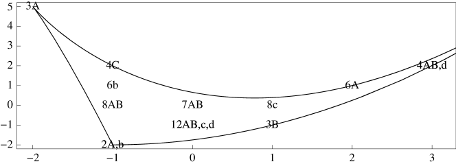
Figure 6.1. The image of the class-set $G_{2}(2)^{\natural}$ inside the class space $G_{2}^{c\natural}$.

We have drawn Figure 6.1 to facilitate the analysis of rigidity in $G_{2}({\mathbb{C}})$. First consider classes which intersect the compact group $G_{2}^{c}$, and are thus represented by points in the closed triangular region drawn in the figure. If $g$ represents one of the vertex classes labeled by $1A$, $3A$, and $2A,b$ respectively, its centralizer has type $G_{2}$, $SL_{3}$, and $SL_{2}\times SL_{2}$, thus dimension $14$, $8$, and $6$ respectively. For $g$ representing a class otherwise on the boundary, the centralizer has type $GL_{2}$ and hence dimension $4$. For $g$ in the interior, the class is regular and so the centralizer dimension is $\mbox{rank}(G_{2})=2$. For general semisimple elements in $G_{2}({\mathbb{C}})$ the situation is the same: centralizer dimensions are $14$, $8$, and $6$ for the three special classes already considered, $4$ for classes on the algebraic curve corresponding to the boundary, and $2$ otherwise.

6.3. $G_{2}$-rigidity of $(3A,3A,3A,4B)$

The first-listed quadruple for $\pi_{1}$ in Prop. 3.1 is $(3A,3A,3A,4B)$. Using the determinations associated to Figure 6.1, the left side of (6.1) becomes $8+8+8+4=28$ which agrees with the right side $(4-2)14=28$. Thus $(3A,3A,3A,4B)$ is $G_{2}$-rigid. We are not pursuing this connection here, but it seems possible to write down a corresponding rank seven differential equation with finite monodromy. From the algebraic solutions to this differential equation, one could perhaps construct the cover $X_{1}\rightarrow U_{3,1,1}$ in a third way.

6.4. Orthogonal rigidity of a lift of $(2A,2A,3A,4A)$

The last-listed quadruple for $\pi_{1}$ in Prop. 3.1 is $(2A,2A,3A,4A)$. This tuple fails to be $G_{2}$-rigid, as now the left side of (6.1) is $6+6+8+3=24$ which is less than $28$. However one does have rigidity of a lift as follows.

The following matrices were sent to me by Stefan Reiter in July 2013.

$$a =\left(\begin{array}[]{rrrrrrr}1&&&&&&\\ &1&&&&&\\ &&1&&&&\\ -3&1&&1&&&\\ 3&-1&&&1&&\\ 9&-3&&&&1&\\ -1&&3&-1&2&-1&1\\ \end{array}\right) \sim\left(\begin{array}[]{rrrrrrr}1&1&&&&&\\ &1&&&&&\\ &&1&1&&&\\ &&&1&&&\\ &&&&1&&\\ &&&&&1&\\ &&&&&&1\\ \end{array}\right)$$

$$b =\left(\begin{array}[]{rrrrrrr}1&&&&3&-1&\\ &1&&&9&-3&\\ &&-2&1&&&\\ &&-9&4&&&\\ &&&&1&&\\ &&&&&1&\\ &&-3&1&&&1\\ \end{array}\right) \sim\left(\begin{array}[]{rrrrrrr}1&1&&&&&\\ &1&&&&&\\ &&1&1&&&\\ &&&1&&&\\ &&&&1&&\\ &&&&&1&\\ &&&&&&1\\ \end{array}\right)$$

$$c =\left(\begin{array}[]{rrrrrrr}1&-1&&&&&-3\\ 3&-2&&&&&\\ &&1&-1&&&3\\ &&3&-2&&&6\\ &&&&1&-1&-3\\ &&&&3&-2&\\ &&&&&&1\\ \end{array}\right) \sim\left(\begin{array}[]{rrrrrrr}\!\omega&&&&&&\\ &\!\omega&&&&&\\ &&\!\omega&&&&\\ &&&\!\overline{\omega}&&&\\ &&&&\!\overline{\omega}&&\\ &&&&&\!\overline{\omega}&\\ &&&&&&1\\ \end{array}\right)$$

$$d =\left(\begin{array}[]{rrrrrrr}10&-5&&&9&-5&-6\\ 15&-8&&&18&-9&-9\\ &&1&&&&\\ -3&4&-3&1&-6&3&3\\ 9&-5&&&10&-5&-6\\ 18&-9&&&15&-8&-9\\ -2&1&&&-2&1&1\\ \end{array}\right) \sim\left(\begin{array}[]{rrrrrrr}1&1&&&&&\\ &1&1&&&&\\ &&1&&&&\\ &&&1&1&&\\ &&&&1&1&\\ &&&&&1&\\ &&&&&&1\\ \end{array}\right)$$

These matrices satisfy $abcd=1$ and they generate a subgroup of $GL_{7}({\mathbb{C}})$ with Zariski closure of the form $G_{2}({\mathbb{C}})$. On the one hand, reduced to $GL_{7}({\mathbb{F}}_{2})$, these matrices generate a copy of $G_{2}(2)^{\prime}$ with $a$, $b$, $c$, and $d$ respectively in $2A$, $2A$, $3A$ and $4A$. On the the other hand, considered in $GL_{7}({\mathbb{C}})$, the matrices have Jordan canonical forms as listed on the right, with $\omega=\exp(2\pi i/3)$.

Consider $a,b,c,d\in G_{2}({\mathbb{C}})\subset SO_{7}({\mathbb{C}})\subset SL_{7}({\mathbb{C}})$. Centralizer dimensions are calculated in [6, §3] and the numerics associated with (6.1) are as follows.

$$\begin{array}[]{c|ccccccccccccc}G&\mbox{cd}_{G}(a)&+&\mbox{cd}_{G}(b)&+&\mbox{cd}_{G}(c)&+&\mbox{cd}_{G}(d)&&&&2\dim(G)\\ \hline\cr G_{2}&8&+&8&+&8&+&4&=&28&=&28\\ SO_{7}&13&+&13&+&9&+&7&=&42&=&42\\ SL_{7}&28&+&28&+&28&+&16&=&90&<&96\end{array}$$

Thus the quadruple $([a],[b],[c],[d])$ is $G_{2}({\mathbb{C}})$- and $SO_{7}({\mathbb{C}})$-rigid. However it is not $SL_{7}({\mathbb{C}})$-rigid, and so does not fit into Katz’s original framework.

Dettweiler and Reiter classify tuples of classes in $G_{2}({\mathbb{C}})$ which are $SO_{7}({\mathbb{C}})$ rigid in [6]. Thus $([a],[b],[c],[d])$ is in their classification. In fact, it appears as the first line of the table in §5.4. Being $SO_{7}({\mathbb{C}})$-rigid is a stronger condition than being $G_{2}({\mathbb{C}})$-rigid. It implies from [6] that there is a corresponding rank seven motive over ${\mathbb{Q}}(p,q)$ with motivic Galois group $G_{2}$.

6.5. Division polynomials and $L$-functions

In §4.3 and §5.5 we have discussed $L$-polynomials $L_{p}(M,x)$ for certain motives $M=H^{1}(\mbox{curve},{\mathbb{Q}})$. Putting these $L$-polynomials together, including also $L$-polynomials at bad primes, one gets a global $L$-function

(6.2) $$L(M,s)=\prod_{p}L_{p}(M,p^{-s})^{-1}.$$

This $L$-function is expected to have standard analytic properties, including an analytic continuation and a functional equation with respect to $s\leftrightarrow 2-s$. Normalizing the motives from §6.3 and §6.4 to have weight $0$, one likewise expects good analytic properties of corresponding $L(M,s)$, involving now functional equations $s\leftrightarrow 1-s$.

We do not know yet how to compute $L$-polynomials in the context of §6.4, where the motivic Galois group is generically the fourteen-dimensional algebraic group $G_{2}$. However the computation of $L$-polynomials is feasible in the setting of §6.3 where the motivic Galois group is just the finite group $G_{2}(2)$. In fact, as commented already in §5.5, we are using motivic language mainly because it is the natural general context for division polynomials. The particular motives from §6.3 correspond to finite-image Galois representations and so this language could be avoided.

In the setting of Section 4, Section 5, and §6.3, analytic computations with global $L$-functions (6.2) are possible on a numerical level. To illustrate this, we consider the motive $M$ from §6.3 associated to the specialization point used in §4.3 and §5.5, namely $(u,v)=(-4,-3)$. This motive corresponds to the seven-dimensional irreducible representation of $G_{2}(2)$ into $SO(7)$. It is natural here to twist by the Dirichlet character $\chi$ given on odd primes $p$ by $\chi(p)=(-1)^{(p-1)/2}$. The twisted motive $M^{\prime}$ corresponding to the other seven-dimensional irreducible representation of $G_{2}(2)$. At the level of good $L$-polynomials, passing back and forth between $M$ and $M^{\prime}$ means replacing $x$ by $\chi(p)x$.

Let $p\geq 5$ be a prime. The corresponding Frobenius class $\mbox{Fr}_{p}$ can usually be deduced from Table 2.1 from the mod $p$ factorization partition of $S_{0}(-4,-3,z)$ and the class of $p$ modulo $4$. To make the necessary distinction between $3A$ and $3B$, we use the factorization partition of the resolvent $f_{36}(4,x)$ presented in (7.2). The $(\chi,\phi)$-coordinates of $\mbox{Fr}_{p}$ on Figure 6.1 then yield the $L$-polynomial

$$L_{p}(M,x)=1-ax+bx^{2}-cx^{3}+cx^{4}-bx^{5}+ax^{6}-x^{7}.$$

Here $a=\chi$, $b=\chi+\phi$, and $c=a+a^{2}-b$.

The necessary $2$-adic and $3$-adic analysis for obtaining conductors and bad $L$-polynomials is begun in Prop. 8.2 below. For $L(M,s)$ the conductor is $2^{20}3^{12}$, the decomposition of the exponents as a sum of seven slopes being as follows.

$$\mbox{At 2: }\;20 =6\cdot 3+2. \mbox{At 3: }\;12 =6\cdot\frac{11}{6}+1.$$

Since all slopes are positive, the bad $L$-polynomials are $L_{2}(M,x)=L_{3}(M,x)=1$. For $L(M^{\prime},s)$, the slopes are all the same except the $2$-adic slope $2$ is now $0$, so that the conductor drops to $2^{18}3^{12}$. Slopes of $0$ contribute to the degree of $L$-polynomials, and in this case $L_{2}(M^{\prime},x)=1-x$ while still $L_{3}(M^{\prime},x)=1$.

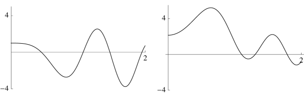
Figure 6.2. Graphs of $L^{*}(M,\frac{1}{2}+it)$ (left) and $L^{*}(M^{\prime},\frac{1}{2}+it)$ (right)

In principle, Magma’s Artin representation and $L$-function packages [2], both due to Tim Dokchister, should do all the above automatically, given simply $S_{0}(-4,-3,z)$ as input. However the inertia groups at $2$ and $3$ are currently too large, and so Magma can only be used with the above extra information at the bad primes. It then outputs numerical values for arbitrary $s$, on the assumption that standard conjectures hold. Particularly interesting $s$ include those of the form $\frac{1}{2}+it$ with $t$ real, i.e. those on the critical line. Here one multiplies $L$ by a phase factor depending analytically on $t$ to obtain a new function $L^{*}$ taking real values only. Figure 6.2 presents plots for our two cases, numerically identifying zeros on the critical line.

To obtain analogous plots of $L^{*}(M,\frac{w+1}{2}+it)$ for a general weight $w$ motive, such as the weight one motives from §4.3 and §5.5, division polynomials do not at all suffice. Here one needs the much more complete information obtained from point counts, like the $L_{p}(M,x)$ presented in §4.3 and §5.5 for $p=5$ and $p=7$. However division polynomials can still be of assistance in obtaining the needed information at the bad primes.

7. Specialization to three-point covers

In §7.1 we find projective lines $P$ in $\overline{U}_{3,1,1}$ and $\overline{U}_{3,2}$ suitably intersecting the discriminant locus in only three points. In §7.2 we consider the covers obtained by the preimages under $\pi_{1}$ and $\pi_{2}$ of these lines. We thereby construct some of the three-point covers $X_{P}\rightarrow P$ mentioned in §3.1. As stated previously, it would be hard to construct these covers directly because these $X_{P}$ always have positive genus. In §7.3 we apply quadratic descent twice to a cover $X_{P}\rightarrow P$ coming from a curve $P\subset U_{3,1,1}$ and recover the Malle-Matzat cover (2.3).

7.1. Curves in $\overline{U}_{3,1,1}$ and $\overline{U}_{3,2}$

The top half of Figure 7.1 is a window on the real points of the naive completion $\overline{U}_{3,1,1}={\mathbb{P}}^{1}_{p}\times{\mathbb{P}}^{1}_{q}$. The discriminant locus ${Z}_{3,1,1}$ consists of the two coordinate axes, the two lines at infinity, and the solution curve $D_{1}$ of

$$p^{2}q^{2}-6pq+4p+4q-3=0.$$

The five lightly drawn straight lines intersect ${Z}_{3,1,1}$ in just three points, not counting multiplicities. The ten other lightly drawn curves have the same three-point property, although it is not visually evident. The points drawn in Figure 7.1 will be discussed in the next section.

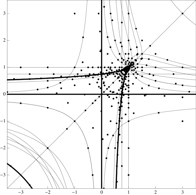
$$\begin{array}[]{lc|cc}\lx@intercol\hfil\lx@intercol\vrule\lx@intercol&p&q\\ \hline\cr G^{\prime}&\bullet&t&1\\ H^{\prime}&\bullet&{8t}/{9}&{3}/{4}\\ I^{\prime}&&(9t-5)/4&{1}/{p^{2}}\\ J^{\prime}&&{(t+3)}/{4}&{(4p-3)/p^{2}}\\ K^{\prime}&a&(t+2)/3&(3p-2)/p^{2}\\ L^{\prime}&e&3(t+4)/16&\!\!9(4p-3)/8p^{2}\!\!\\ F^{*}&\bullet f&{3}/{(4t-1)}&{3}/(4t-1)\\ M^{*}&&t&1/t\\ B^{*}&b&-3t&-{3}/{t}\end{array}\;\;\;\;\;\;\begin{array}[]{cc|cc}\lx@intercol\hfil\hfil\lx@intercol\vrule\lx@intercol&p&q\\ \hline\cr G^{\prime\prime}&\bullet&1&t\\ H^{\prime\prime}&\bullet&3/4&8t/9\\ I^{\prime\prime}&&{1/q^{2}}&(9t-5)/4\\ J^{\prime\prime}&&{(4q-3)}/{q^{2}}&{(t+3)}/{4}\\ K^{\prime\prime}&c&(3q-2)/{q^{2}}&(t+2)/3\\ L^{\prime\prime}&d&\!\!9(4q-3)/8q^{2}\!\!&3(t+4)/16\\ \lx@intercol\hfil\hfil\lx@intercol\\ \lx@intercol\hfil\hfil\lx@intercol\\ \lx@intercol\hfil\hfil\lx@intercol\\ \end{array}$$

Figure 7.1. Top: The $p$-$q$ plane $U_{3,1,1}({\mathbb{R}})$. Discriminant loci (thick), bases of three-point covers (thin), and specialization points are drawn in. Bottom: parametrizations of the bases for three-point covers

The bottom half of Figure 7.1 names and parametrizes the fifteen lightly drawn curves in the top half. Each name is a superscripted letter. The five bulleted curves are the straight lines. There are other natural coordinate systems on the $p$-$q$-plane, and each of the other curves appears as a line in at least one of these coordinate systems. We are emphasizing the coordinates $p$ and $q$ because they make the natural involution of $U_{3,1,1}$ completely evident as $p\leftrightarrow q$. The three curves labeled $T^{*}$ are stable under this involution. The remaining twelve curves form six interchanged pairs: $T^{\prime}\leftrightarrow T^{\prime\prime}$. Six of the fifteen curves are images of lines in the cubic cover $U$. These source lines in $U$ are indicated by $a$, $b$, $c$, $d$, $e$, and $f$.

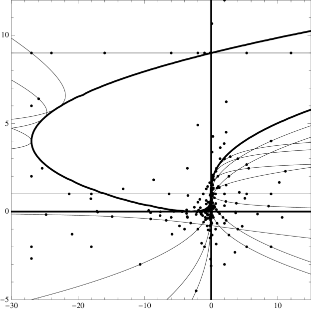
$$\begin{array}[]{l|cc}&a&b\\ \hline\cr A&-{27(b-1)^{3}}/{(5b-9)}&9(t-1)/{(5t-9)}\\ B\bullet&-48(t-1)&9\\ C&-(b-9)(5b-9)/27&9(t-1)/{(5t-1)}\\ E&-{(b-1)^{3}}/{(b-3)}&{3(t-1)}/{(t-3)}\\ F&-{3}/{\left(9t^{2}-7t+1\right)^{2}}&\frac{9(t-1)t}{9t^{2}-7t+1}\\ M\bullet&-16t&1\end{array}\;\;\;\;\;\;\begin{array}[]{l|cc}&a&b\\ \hline\cr G&(b-1)^{2}&t\\ H&b(3b-2)/3&{2t}/{3}\\ I&{(b-1)^{2}(5b+4)/b}&{4}/{(9t-5)}\\ J&-{(b-1)^{2}b/3(b-4)}&{4t}/{(t+3)}\\ K&-{(b-1)^{3}}/{(b-3)}&{3t}/{(t+2)}\\ L&\frac{-b^{2}(10b-9)}{27(2b-9)}&{9t}/{2(t+4)}\\ \end{array}$$

Figure 7.2. Top: The $a$-$b$ plane $U_{3,2}({\mathbb{R}})$. Discriminant loci (thick), bases of three-point covers (thin), and specialization points are drawn in. Bottom: parametrizations of the bases for three-point covers.

Figure 7.2 is the analog of Figure 7.1 for $\overline{U}_{3,2}={\mathbb{P}}^{2}_{a,b}$ and we will describe it more briefly, focusing on differences. The discriminant locus $Z_{3,2}$ has four components, the two coordinate axes, the line at infinity, and the curve $D_{2}$ with equation

$$a^{2}-2ab^{2}+12ab+6a+b^{4}-12b^{3}+30b^{2}-28b+9=0.$$

The light curves each intersect the discriminant locus in three points, where this time a contact point with $D_{2}$ does not count if the local intersection number is even. Despite the relaxing of the three-point condition, we have found only twelve such curves. The five curves $A$, $B$, $C$, $E$, and $F$ are images of generically bijective maps from curves $a$, $b$, $c$, $e$, and $f$ in $U$. Curve $d$ in $U$ double covers $B$, and so does not have its own entry on Figure 7.2. For $T=G$, $H$, $I$, $J$, $K$, and $L$, the curve $T\subset U_{3,2}$ comes from $T^{\prime}$ and $T^{\prime\prime}$ in $U_{3,1,1}$ via (3.1). Finally $M\subset U_{3,2}$ is double-covered by $M^{*}$ in $U_{3,1,1}$.

7.2. Three-point covers with Galois group $\Gamma.2$

The previous subsection concerned the base varieties $U_{3,1,1}$ and $U_{3,2}$ only. For quite general covers $X\rightarrow U_{\nu}$, one gets three-point covers $X_{P}\rightarrow P$ by specialization to the $P\subset X_{\nu}$ listed there. We now apply this theory to our particular covers $\pi_{1}:X_{1}\rightarrow U_{3,1,1}$ and $\pi_{2}:X_{2}\rightarrow U_{3,2}$. Because of the explicit parametrizations in Figures 7.1 and 7.2, our bases are now coordinatized projective lines ${\mathbb{P}}^{1}={\mathbb{P}}^{1}_{t}$.

$$\begin{array}[]{ccc|ccc|cr|cc}X_{0}&X_{311}&X_{32}&C_{0}&C_{1}&C_{\infty}&g_{28}&g_{36}&\bar{\mu}&\mu\\ \hline\cr&H^{\prime\prime}&&4A&4B&3B&-&-&0.\overline{3}&0\\ &I^{\prime\prime}&&4A&12A&2A&-&-&0.\overline{3}&0\\ \hline\cr b&B^{*}&B&6A&2A&8A&1&0&1&1\\ \hline\cr&&M&12A&2A&8B&2&2&1&1\\ &&G&4A&6A&3B&2&2&1&1\\ &H^{\prime},G^{\prime\prime}&&12A&4A&3B&2&5&1&1\\ \hline\cr e&L^{\prime}&E,K&4C&4A&8A&3&3&1&1\\ &G^{\prime}&H&3A&12A&3B&3&5&1&1\\ \hline\cr a&K^{\prime}&A&4A&8A&8B&4&7&1&1\\ c&K^{\prime\prime}&C,I&3A&8A&6A&4&6&1&1\\ d&L^{\prime\prime}&&6A&4A&6A&4&5&1&1\\ \hline\cr f&F^{*},I^{\prime}&F&4A&8B&12B&5&8&1&1\\ &J^{\prime}&&4A&12A&8B&5&8&1&1\\ &&L&12A&3A&8A&5&8&1&1\\ \hline\cr&M^{*}&J&6A&12A&8B&7&10&5&5\\ \hline\cr&J^{\prime\prime}&&12A&12A&6A&8&11&4.08\overline{3}&3\\ \end{array}$$

Table 7.1. Sixteen three-point covers obtained from $\pi_{1}$ and $\pi_{2}$ by specialization

Table 7.1 gives the results. The first two lines illustrate the general phenomenon where Galois groups sometimes become smaller under specialization. Here the covers have Galois groups of order $216$ and $432$ respectively, thus of index $56$ and $28$ in $\Gamma.2$. The covers $X_{28}\rightarrow{\mathbb{P}}^{1}$ each split into a genus one cover $X_{27}\rightarrow{\mathbb{P}}^{1}$ and the trivial cover ${\mathbb{P}}^{1}\rightarrow{\mathbb{P}}^{1}$.

The next fourteen lines each give a cover $X_{28}\rightarrow{\mathbb{P}}^{1}$ with Galois group all of $\Gamma.2$. They are sorted by the genus $g_{28}$ of this cover. In most cases, more than one base curve ${\mathbb{P}}^{1}$ yield isomorphic covers, after suitable permutations of the three cusps $\{0,1,\infty\}$. The local monodromy classes in $\Gamma$ always correspond to the first-listed parametrized base. These classes are unambiguously determined, except for a simultaneous interchange $4A\leftrightarrow 4B$, $8A\leftrightarrow 8B$, $12A\leftrightarrow 12B$, coming from the outer automorphism of $\Gamma$. We always normalize by making the first-listed interchanged class have an $A$ is its name.

Thus for example, specializing $S_{1}(p,q,x)$ at $(p,q)=(-3t,-3/t)$ from the $B^{*}$ line of Figure 7.1, one gets a polynomial in ${\mathbb{Z}}[t,x]$ with $554$ terms. The local monodromy partitions are $(6A,2A,8A)$ as printed. Alternatively, specializing $S_{2}(a,b,x)$ at $(a,b)=(-48(t-1),9)$ from the $B$ line of Figure 7.2, one gets a polynomal in ${\mathbb{Z}}[t,x]$ now with $252$ terms. The monodromy partitions are the same, except for the reordering $(C_{0},C_{1},C_{\infty})=(2A,6A,8A)$.

Having specialized from two parameters down to one, it is now much more reasonable to print polynomials giving equations $f_{28}(t,x)=0$ and $f_{36}(t,x)=0$ corresponding to the covers in any of the last fourteen lines of Table 7.1. We do this only in the case where genera are the smallest, namely the third line:

$$f_{28}(t,x)=$$

$$-t\left(3x^{4}-252x^{3}+222x^{2}-692x-5\right)\cdot$$

$$\qquad\left(81x^{12}+2106x^{11}+26001x^{10}+73332x^{9}+268515x^{8}+574938x^{7}\right.$$

$$\qquad\left.+618759x^{6}+400896x^{5}+184140x^{4}+52752x^{3}+8952x^{2}+576x-32\right)^{2}$$

$$+2^{10}(1-t)(4x+1)\left(9x^{4}+18x^{3}+48x^{2}+18x+1\right)^{6}$$

$$+3^{9}(1-t)t(x-2)^{8}x^{2}\left(x^{2}+8\right)\left(x^{2}-2x-1\right)^{8},$$

(7.2) $$f_{36}(t,x)=$$

$$\qquad\left(4x^{4}-3\right)^{3}\left(4x^{4}-12x^{2}+12x-3\right)^{6}$$

$$\qquad-3^{9}t(x-1)^{4}\left(2x^{2}-1\right)^{8}\left(2x^{2}-2x+1\right)^{4}.$$

Here the genera, namely $(g_{28},g_{36})=(1,0)$ are the reverse of those of the Malle-Matzat covers.

7.3. Recovering the Malle-Matzat curve

The Malle-Matzat cover can be constructed from the last line of Table 7.1 via two quadratic descents as follows. The given cover $X_{1}\rightarrow{\mathbb{P}}_{t}^{1}$ has ramification invariants $(12A,12A,6A)$. Quotienting out by the involution $t\leftrightarrow 1-t$ on the base and its unique lift to $X_{1}$, one gets the descended cover $X_{2}\rightarrow{\mathbb{P}}_{s}^{1}$, with $s=4t(1-t)$. The ramification invariants of this cover are $(12A,2A,12B)$. Quotienting now by $s\leftrightarrow 1/s$ on the base and its unique lift to $X_{2}$, one gets the twice descended cover $X_{3}\rightarrow{\mathbb{P}}^{1}_{u}$, with $u=-(s-1)^{2}/4s$. The ramification invariants of this cover are $(4b,2b,12AB)$, showing that it is the Malle-Matzat cover.

In other words,

$$m\left(\frac{(2t-1)^{4}}{16(t-1)t},x\right)\mbox{ and }S_{1}\left(\frac{16t}{(t+3)^{2}},\frac{t+3}{4},z\right)$$

are two different polynomials defining the same degree 28 extension of ${\mathbb{Q}}(t)$. The left one is a quartic base-change of the Malle-Matzat polynomial $m(u,x)$ while the right is a specialization of $S_{1}(p,q,x)$.

8. Specialization to number fields

In this final section, we discuss specialization to number fields with discriminant of the form $2^{j}3^{k}$. §8.1 discusses fields obtained by specializing the $\pi_{i}$. §8.2 continues this discussion, involving also similar fields from other sources. §8.3 discusses analysis of ramification in general, with a field having Galois group $PGL_{2}(7)$ serving as an example. §8.4 concludes by analyzing the ramification of a particularly interesting field with Galois group $SU_{3}(3).2\cong G_{2}(2)$.

8.1. Specializing the covers $\pi_{i}$

In this subsection, we restrict attention to number fields with Galois group $\Gamma.2$ and discriminant of the form $2^{j}3^{k}$. Consider first the cover $X_{0}\rightarrow U$. We have found 216 ordered pairs $(u,v)$ such that the corresponding number field ${\mathbb{Q}}[x]/F_{0}(u,v,x)$ has Galois group $\Gamma.2$ and discriminant of the form $2^{j}3^{k}$. Different specialization points can give isomorphic fields, and we found 147 number fields in this process.

Next consider the covers $\pi_{1}:X_{1}\rightarrow U_{3,1,1}$ and $\pi_{2}:X_{2}\rightarrow U_{3,2}$. Beyond images of specialization points in $U({\mathbb{Q}})$, we found 248 pairs $(p,q)$ and 177 pairs $(a,b)$ giving fields with Galois group $\Gamma.2$ and discriminant of the form $2^{j}3^{k}$. We obtained 62 new fields arising from both covers, 95 new fields arising from $\pi_{1}$ only, and 72 new fields arising from $\pi_{2}$ only. Thus we found in total 376 fields with Galois group $\Gamma.2$ and discriminant of the form $2^{j}3^{k}$.

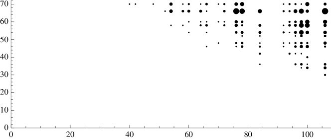
Figure 8.1. Pairs $(j,k)$ arising from field discriminants $2^{j}3^{k}$ from specializations of $F_{1}(p,q,x)$ and $F_{2}(a,b,x)$

Figure 8.1 indicates the pairs $(j,k)$ arising from field discriminants $2^{j}3^{k}$ of one of these 376 fields. The area of the disk at $(j,k)$ is proportional to the number of fields giving rise to $(j,k)$. In $36$ cases, this field is unique. The largest multiplicity is $19$, arising from $(j,k)=(106,66)$. The smallest discriminant is $2^{66}3^{46}$, coming from just one field. This field arises from eight sources,

$$(u,v) =(-4,-3),(-\frac{1}{2},1),(\frac{1}{2},3),(4,-3),(-32,1),(-\frac{32}{81},\frac{49}{81}),$$

(8.1) $$(p,q) =(1,\frac{1}{2}),$$

$$(a,b) =(-\frac{27}{4},-\frac{1}{2}).$$

The largest discriminant $2^{106}3^{70}$ arises from four fields.

The phenomenon of several specialization points giving rise to a single field is quite common in our collection of covers $\pi_{i}$. The octet in (8.1) is the most extreme instance, but there are many other multiplets as altogether $216+248+177=641$ different specialization points give rise to only 376 fields. This repetition phenomenon is discussed for a different cover in [14, §6], where it is explained by a Hecke operator. It would be of interest to give a similar automorphic explanation of the very large drop $641\rightarrow 376$. Ideally, such a description would follow through on one of the main points of view of Deligne and Mostow [4, 5], by describing all our surfaces via uniformization by the unit ball in ${\mathbb{C}}^{2}$.

8.2. Summary of known fields

We specialized the Malle-Matzat cover in [14, §8] to obtain fields with discriminant of the form $2^{j}3^{k}$. From $t=1/2$ we obtained a field with Galois group $\Gamma$, while from $41$ other $t$ we obtained $41$ other fields with Galois group $\Gamma.2$. While in our covers $\pi_{i}$ the $.2$ always corresponds to the quadratic field ${\mathbb{Q}}(i)$, in the Malle-Matzat cover general ${\mathbb{Q}}(\sqrt{\partial})$ arise.

Sorting all the known fields by $\partial\in{\mathbb{Q}}^{\times}/{\mathbb{Q}}^{\times 2}$, including two additional fields from [15] with $\partial=2$ and $\partial=6$, one has the following result.

Proposition 8.1.

There are at least $409$ degree twenty-eight fields with Galois group $\Gamma$ or $\Gamma.2$ and discriminant of the form $2^{j}3^{k}$. Sorted by the associated quadratic algebra ${\mathbb{Q}}[x]/(x^{2}-\partial)$, these lower bounds are

$$\begin{array}[]{c|cccccccl}\partial&-6&-3&-2&-1&1&2&3&6\\ \hline\cr\#&5&6&6&381&1&7&2&1.\end{array}$$

Two aspects of our incomplete numerics are striking. First, it is somewhat surprising that there are at least $408$ number fields with Galois group $\Gamma.2$ and discriminant $2^{j}3^{k}$. By way of contrast, the number of fields with Galois group $S_{7}$, $S_{8}$, and $S_{9}$ and discriminant $\pm 2^{j}3^{k}$ is exactly $10$, at least $72$, and at least $46$ respectively [9]. Second, the imbalance with respect to $\partial$ is quite extreme. We have not been exhaustive in specializing our covers and we expect that the $381$ could be increased somewhat. By exhaustively specializing Shioda’s $W(E_{7})^{+}$ family, in principle one could obtain the correct values on the bottom row. Our expectation however is that most fields have already been found and so the imbalance favoring ${\mathbb{Q}}(i)$ is maintained in the complete numerics.

8.3. Analysis of ramification

In general, let $K$ be a degree $n$ number field with discriminant $d$ and root discriminant $\delta=|d|^{1/n}$. It is important to simultaneously consider the Galois closure $K^{\rm gal}$, its discriminant $D$ and its root discriminant $\Delta=|D|^{1/N}$. For a given field $K$, one has $\delta\leq\Delta$. To emphasize the fact that the large field $K^{\rm gal}$ is never directly seen in computations, we call $\Delta$ the Galois root discriminant or GRD of $K$. A GRD $\Delta$ is typically much harder to compute than the corresponding root discriminant $\delta$, as it requires good knowledge of higher inertia groups at each ramifying prime.

For sufficiently simple $K$, ramification is thoroughly analyzed by the website associated to [7], and the GRD $\Delta$ is automatically computed. The 409 fields $K$ contributing to Proposition 8.1 are not in the simple range, and we will present one ad hoc computation of a GRD $\Delta$ in the next subsection. As an illustration of the general method, we first consider an easier case here.

For the easier case, take $t=-1$ in (7.2), which corresponds to $(p,q)=(3,3)$ via $B^{*}$ and $(a,b)=(-48,9)$ via $B$, both of which come from $(u,v)=(1,2)$. The discriminant and root discriminant of $K={\mathbb{Q}}[x]/f_{28}(-1,x)$ are $d=2^{92}3^{24}$ and $\delta\approx 25.007$ respectively. This root discriminant is much smaller than the minimum $(2^{66}3^{46})^{1/28}\approx 31.147$ appearing in §8.1. The field $K$ was excluded from consideration in §8.1 because the Galois group is not $\Gamma.2$ but rather the $336$-element subgroup $PGL_{2}(7)$. This drop in Galois group is confirmed by the factorization of the resolvent into irreducibles: $f_{36}(-1,x)=xf_{14}(x)f_{21}(x)$.

The group $PGL_{2}(7)$ can be embedded in $S_{8}$, which means that $K^{\rm gal}$ can also be given as the splitting field of a degree eight polynomial. Such a degree eight polynomial was already found in [8, Table 8.2]:

$$f(x)=x^{8}-6x^{4}-48x^{3}-72x^{2}-48x-9.$$

The analysis of ramification is then done automatically by the website associated to [7], returning for each prime $p$ a slope content symbol $SC_{p}$ of the form $[s_{1},\dots,s_{k}]_{t}^{u}$. This means that the decomposition group $D_{p}$ has order $p^{k}tu$, the inertia subgroup $I_{p}$ has order $p^{k}t$, and the wild inertia subgroup $P_{p}$ has order $p^{k}$. The wild slopes $s_{i}$ are then rational numbers greater than one measuring wildness of ramification, as explained in [7, §3.4].

In our $PGL_{2}(7)$ example, also taking weighted averages to get Galois mean slope [7, §3.7], the result is

$$SC_{2} =[2,3,7/2,9/2]_{1}^{1}, GMS_{2} =\frac{1}{16}\cdot 2+\frac{1}{8}\cdot 3+\frac{1}{4}\cdot\frac{7}{2}+\frac{1}{2}\cdot\frac{9}{2}=\frac{29}{8},$$

$$SC_{3} =[\;]_{7}^{6}, GMS_{3} =\frac{6}{7}.$$

The Galois root discriminant is then $\Delta=2^{29/8}3^{6/7}\approx 31.637$. This Galois root discriminant is the fifth smallest currently on [9] from a field with Galois group $PGL_{2}(7)$.

8.4. A lightly ramified number field

Let $K$ be the number field coming from the eight specialization points (8.1). Applying Pari’s polredabs [13] to get a canonical polynomial, this field is $K={\mathbb{Q}}[x]/f(x)$ with

$$f(x)=$$

$$x^{28}-4x^{27}+18x^{26}-60x^{25}+165x^{24}-420x^{23}+798x^{22}-1440x^{21}+2040x^{20}$$

$$-2292x^{19}+2478x^{18}-756x^{17}-657x^{16}+1464x^{15}-4920x^{14}+3072x^{13}$$

$$-1068x^{12}+3768x^{11}+1752x^{10}-4680x^{9}-1116x^{8}+672x^{7}+1800x^{6}-240x^{5}$$

$$-216x^{4}-192x^{3}+24x^{2}+32x+4.$$

The field $K$ arises from (7.2) with either $t=4$ or $t=32/81$, so we also have its resolvent $K_{36}={\mathbb{Q}}[x]/f_{36}(4,x)$ from (7.2). Since one of the eight specialization points in (8.1) is $(u,v)=(-4,-3)$, we have also seen this field already in the three subsections about $L$-polynomials, §4.3, §5.5, and §6.5.

Let $K^{\rm gal}$ be the splitting field of $K$. Calculation of slope contents is not automatically done by the website of [7] because degrees are too large. The proof of the following proposition illustrates the types of considerations which are built into [7] for smaller degrees.

Proposition 8.2.

The decomposition groups of $K^{\rm gal}$ at the ramified primes have invariants as follows:

$$SC_{2} =[2,2,2,3,3]_{1}^{3}, GMS_{2} =\frac{7}{32}\!\cdot\!2+\frac{3}{4}\!\cdot\!3=\frac{43}{16},$$

$$SC_{3} =[13/8,13/8,11/6]_{8}^{2}, GMS_{3} =\frac{1}{27}\!\cdot\!\frac{7}{8}+\frac{8}{27}\!\cdot\!\frac{13}{8}+\frac{2}{3}\!\cdot\!\frac{11}{6}=\frac{125}{72}.$$

Thus the root discriminant of $K^{\rm gal}$ is $\Delta=2^{43/16}3^{125/72}\approx 43.386$.

Proof.

The computation is easier at the prime $p=3$ and so we do it first. The field $K$ factors $3$-adically as $K_{27}\times{\mathbb{Q}}_{3}$ with $K_{27}$ having discriminant $3^{46}$. The exponent arises from three slopes $s_{1}\leq s_{2}\leq s_{3}$ via $46=2s_{1}+6s_{2}+18s_{3}$. One of the two degree $63$ resolvents, computed by Magma, factors $3$-adically as $K_{54}\times K_{9}$, with $K_{9}\cong{\mathbb{Q}}_{3}[x]/(x^{9}+6x^{5}+6)$ having slope content $[13/8,13/8]_{8}^{2}$. This forces the remaining slope of $K_{27}$ to be $s_{3}=11/6$. The inertia group $D_{3}$ is thus the maximal subgroup $3_{+}^{1+2}:8:2$ of $\Gamma.2$, with slope content $[13/8,13/8,11/6]_{8}^{2}$.

Moving on to the prime $2$, the field $K$ factors $2$-adically as $K_{16}\times K_{12}$. Here $K_{16}$ is totally ramified of discriminant $2^{42}$. The complement $K_{12}$ contains the unramified cubic extension of ${\mathbb{Q}}_{2}$ and has discriminant $2^{24}$. Since the group $S_{16}\times(S_{4}\wr C_{3})$ does not contain an element of cycle structure either $8^{3}21$ or $8^{3}4$, the decomposition group $D_{2}$ cannot contain an element of order eight. So even though $\mbox{ord}_{2}(|\Gamma.2|)=6$, there can be at most five wild slopes.

The resolvent $K_{36}$ factors as $K_{16}\times K_{12}\times K_{8}$, with $K_{8}\cong{\mathbb{Q}}_{2}[x]/(x^{8}+2x^{7}+2)$ having discriminant $2^{14}$ and slope content $[2,2,2]_{1}^{3}$. Thus we have found three slopes to be $2$, $2$, and $2$. If we can find two more wild slopes we will have identified all wild slopes.

The field $K_{8}$ and the sextic field $K_{6}={\mathbb{Q}}_{2}[x]/(x^{6}+x^{2}+1)$ with discriminant $2^{6}$ have the same splitting field. The latter is a subfield of $K_{12}$ showing that $(24-6)/6=3$ is a fourth $2$-adic slope. In fact, since both involutions in $\Gamma.2$ have cycle type $2^{12}1^{4}$ and therefore must appear in the degree $12$ factor, $3$ is the largest wild slope.

The quartic subfield of $K_{8}$ is $K_{4}={\mathbb{Q}}_{2}[x]/(x^{4}+2x^{3}+2x^{2}+2)$ with discriminant $2^{6}$. Computation shows it is a subfield of $K_{16}$. So the remaining slope $s$ satisfies $1\!\cdot\!2+2\!\cdot\!2+4\!\cdot\!s+8\!\cdot\!3=42$ and must also be $3$. The tame degree $I_{2}/P_{2}$ can only be $1$, as the only other possibility $t=3$ would force $u=2$ and $\Gamma.2$ does not contain a solvable subgroup of order a multiple of $2^{6}3^{2}=576$. Thus $D_{2}$ has order $96$ and slope content $[2,2,2,3,3]_{1}^{3}$. ∎

The Galois root discriminant $\Delta\approx 43.386$ is very low, as is clear from the discussion in [8], as updated in [9, Table 9.1]. In fact, the field $K^{\rm gal}$ is a current record-holder, in the sense that all known Galois fields with smaller root discriminants involve only simple groups of size smaller than 6048 in their Galois groups.

References

- [1] Y. André, Une introduction aux motifs (motifs purs, motifs mixtes, périodes), Panoramas et Synthèses, 17, Soc. Math. de France, Paris, 2004. xii+261 pp.
- [2] W. Bosma, J. J. Cannon, C. Fieker, A. Steel (eds.), Handbook of Magma functions, Edition 2.19 (2012).
- [3] J. H. Conway, R. T. Curtis, S. P. Norton, R. A. Parker, R. A. Wilson, Atlas of finite groups. Oxford University Press, 1985.
- [4] P. Deligne and G. D. Mostow. Monodromy of hypergeometric functions and nonlattice integral monodromy, Inst. Hautes Études Sci. Publ. Math. No. 63 (1986), 5–89.
- [5] by same authorCommensurabilities among lattices in , Annals of Mathematics Studies, 132, Princeton University Press, Princeton, NJ, 1993. viii+183 pp.
- [6] M. Dettweiler and S. Reiter, The classification of orthogonally rigid -local systems and related differential operators, Trans. Amer. Math. Soc. 366 (2014), no. 11, 5821–5851.
-
[7]
J. W. Jones and D. P. Roberts, A database of local fields,
J. Symbolic Comput. 41 (2006), no. 1, 80–97. Database at
http://math.la.asu.edu/~jj/localfields/ - [8] by same authorGalois number fields with small root discriminant, J. Number Theory 122 (2007), no. 2, 379–407.
-
[9]
by same authorA database of number fields, to appear in London Math. Soc. J. of Comp. and Math., Arxiv 1404.0266. Database at
http://hobbes.la.asu.edu/NFDB/ - [10] N. M. Katz, Rigid local systems, Annals of Mathematics Study 138, Princeton University Press (1996).
- [11] G. Kemper, Generic polynomials are descent-generic, Manuscripta Math. 105 (2001), no. 1, 139–141.
- [12] G. Malle and B. H. Matzat. Inverse Galois Theory. Springer-Verlag, 1999.
- [13] The PARI group, Bordeaux. PARI/GP. Version 2.3.4, 2009.
- [14] D. P. Roberts, An construction of number fields, Number theory, 237–267, CRM Proc. Lecture Notes, 36, Amer. Math. Soc., Providence, RI, 2004.
- [15] by same authorCovers of and number fields, in preparation.
- [16] T. Shioda, Theory of Mordell-Weil lattices, Proceedings of the International Congress of Mathematicians, Vol. I, II (Kyoto, 1990), 473–489, Math. Soc. Japan, Tokyo, 1991.
- [17] by same authorPlane quartics and Mordell-Weil lattices of type . Comment. Math. Univ. St. Paul. 42 (1993), no. 1, 61–79.
- [18] H. Weber, Lehrbuch der Algebra III, 3rd ed., Chelsea, New York, 1961.
- [19] Wolfram Research, Inc., Mathematica, Version 10.0, Champaign, IL (2014).