Hyperelliptic uniformization
of algebraic curves of the third order

Abstract

An algebraic function of the third order plays an important role in the problem of asymptotics of Hermite-Padé approximants for two analytic functions with branch points. This algebraic function appears as the Cauchy transform of the limiting measure of the asymptotic distribution of the poles of the approximants. In many cases this algebraic function can be determined by using the given position of the branch points of the functions which are approximated and by the condition that its Abelian integral has purely imaginary periods. In the present paper we obtain a hyperelliptic uniformization of this algebraic function. In the case when each approximated function has only two branch points, the genus of this function can be equal to $0$, $1$ (elliptic case) or $2$ (ultra-elliptic case). We use this uniformization to parametrize the elliptic case. This parametrization allows us to obtain a numerical procedure for finding this elliptic curve and as a result we can describe the limiting measure of the distribution of the poles of the approximants.

Dedicated to our friend Pablo González Vera

Keywords: Multiple orthogonal polynomials; Hermite-Padé rational approximants; Riemann surfaces; Algebraic functions; Uniformization.

AMS subject classification: Primary 33C45, 41A21, 42C05.

1 Introduction

1.1 Definition of Hermite-Padé approximants and motivation of the problem

This paper is devoted to the analysis of an algebraic curve. This curve plays an important role in the analytic theory of Hermite-Padé approximants. We start with their definition.

Let $\vec{f}=(f_{1},\ldots,f_{p})$ be a vector of $p$ Laurent series near infinity

$$f_{j}(z)=\sum_{k=0}^{\infty}\frac{f_{j,k}}{z^{k}},\qquad j=1,\ldots,p.$$ (1.1)

The Hermite-Padé rational approximants (of type II)

$$\pi_{\vec{n}}=\left(\frac{Q_{\vec{n}}^{(1)}}{P_{\vec{n}}},\ldots,\frac{Q_{\vec{n}}^{(p)}}{P_{\vec{n}}}\right)$$

for the vector $\vec{f}$ and multi-index $\vec{n}=(n_{1},\ldots,n_{p})\in\mathbb{N}^{p}$ are defined by

$$\deg P_{\vec{n}}\leq|\vec{n}|=n_{1}+\cdots+n_{p}\,,\qquad P_{\vec{n}}\not\equiv 0,$$

$$f_{j}(z)P_{\vec{n}}(z)-Q_{\vec{n}}^{(j)}(z)=:R_{\vec{n}}^{(j)}(z)=\mathcal{O}\left(\frac{1}{z^{n_{j}+1}}\right),\qquad z\to\infty,$$ (1.2)

where the $Q_{\vec{n}}^{(j)}$ are polynomials, for $j=1,\ldots,p$. This definition is equivalent to a homogeneous linear system of equations for the coefficients of the polynomial $P_{\vec{n}}$. This system always has a solution, but the solution is not necessarily unique. In the case of uniqueness (up to a multiplicative constant) and in case every non-trivial solution has full degree $\vec{n}$, the multi-index $\vec{n}$ is called normal and the polynomial $P_{\vec{n}}$ can be normalized to be monic

$$P_{\vec{n}}(z)=\prod_{k=1}^{|\vec{n}|}(z-z_{k,\vec{n}}).$$

The Hermite-Padé approximants $\pi_{\vec{n}}$ provide the best local (at infinity) simultaneous rational approximation of the vector $(f_{1},\ldots,f_{p})$ of the Laurent series (1.1) with a common denominator. The construction (1.2) was introduced by Hermite [9] in connection with his proof of the transcendence of $e$. See the papers [11, 1, 17] for more details.

A key problem in the study of the analytical properties (convergence, asymptotics) of the diagonal (i.e., $\vec{n}=(n,\ldots,n)$) Hermite-Padé approximants is to determine the limiting distribution of the zeros of the common denominator $P_{\vec{n}}$, which are the poles of the Hermite-Padé approximants, i.e., to determine the weak-$\ast$ limit of the discrete measures

$$\nu_{P_{\vec{n}}}=\frac{1}{n}\sum_{k=1}^{pn}\delta(z-z_{k,\vec{n}}),\qquad n\to\infty.$$ (1.3)

A class of analytic functions $\{f_{j}\}_{j=1}^{p}$ with a finite number of branch points plays an important role in recent investigations. We denote the sets of the branch points of the functions $f_{j}$ by $A_{j},\,\,j=1,\ldots,p$. We say that

$$f_{j}\in\mathcal{A}(\overline{\mathbb{C}}\setminus A_{j}),\quad\sharp A_{j}<\infty,\quad A_{j}\subset\mathbb{C},\quad j=1,\ldots,p$$

if the Laurent expansion (1.1) is convergent in a neighborhood of infinity and has an analytic continuation along any path in the complex plane $\mathbb{C}$ avoiding the sets $A_{j}$ of the branch points.

In accordance with Nuttall’s conjecture (see [11]) the limit of the zero counting measures (1.3) exists

$$\nu_{P_{\vec{n}}}\stackrel{{\scriptstyle*}}{{\to}}\lambda,$$

and the Cauchy transform of $\lambda$ (after analytic continuation) is an algebraic function of order $p+1$. We denote this function by $h$ and we denote the algebraic Riemann surface of $h$ by $\mathfrak{R}$. The function $h$ has branches $h_{0}(z),h_{1}(z),\ldots,h_{p}(z)$ which at infinity behave as

$$h_{0}(z)=-\frac{p}{z}+\mathcal{O}(z^{-2}),\qquad h_{j}(z)=\frac{1}{z}+\mathcal{O}(z^{-2}),\quad j=1,\ldots,p.\qquad z\to\infty.$$ (1.4)

In particular, the conjecture states that the branch $h_{0}$ (fixed at infinity) is the Cauchy transform of the limiting zero counting measure

$$h_{0}(z)=\int\frac{d\lambda(x)}{x-z}\,,\qquad z\in\overline{\mathbb{C}}\setminus\mbox{Supp}(\lambda).$$

Moreover, the conjecture describes the strong asymptotics of the Hermite-Padé approximants (1.2) using Riemann-Hilbert boundary problems on the Riemann surface $\mathfrak{R}$. However, a still unsolved problem is how to find (for a general setting) the main ingredient of the Nuttall conjecture, i.e., the Riemann surface $\mathfrak{R}$.

In [2] a potential theory approach to define a corresponding Riemann surface $\mathfrak{R}$ for the case of two functions with a finite number of branch points was suggested. The potential theory approach was proposed for the first time in [8] for real analytic functions with real sets of branch points $A_{j}$ and nonintersecting intervals $\Delta_{j}$, which are the convex hulls of $A_{j}$

$$A_{j}\subset\Delta_{j}\subset\mathbb{R},\qquad\Delta_{j}\cap\Delta_{k}=\emptyset,\quad 1\leq j\neq k\leq p.$$

An approach based on the notion of Nuttall’s condenser was proposed recently by Rakhmanov and Suetin in [13].

The investigation of the asymptotic behavior of the diagonal Hermite-Padé approximants for two functions

$$f_{j}\in\mathcal{A}(\overline{\mathbb{C}}\setminus A_{j}),\quad A_{j}=\{a_{j},b_{j}\},\,\,j=1,2$$ (1.5)

was started in [4]. A typical example consists of the functions $f_{j}(z)=\log((z-a_{j})/(z-b_{j})),\,\,j=1,2$. Only the case where the dispositions of the branch points of $f_{1}$ and $f_{2}$ lead to a corresponding Riemann surface $\mathfrak{R}$ of genus zero was studied in [4]. A complete characterization of algebraic curves of the third order, and of genus zero, which have the fixed projections $A_{j}=\{a_{j},b_{j}\},\,\,j=1,2$ of the branch points, was carried out in [5], [3], (see also [10]).

In this paper, as in [4], we consider the case of two pairs of branch points (1.5) and, in order to describe the asymptotics of the Hermite-Padé approximants, we investigate a numerical procedure for finding the equation of the algebraic Riemann surface $\mathfrak{R}$ of genus higher than zero.

Throughout the paper we use the following notation, conventions and definitions. We denote the branches of a multi-valued function $h$ by $h_{0}(z),h_{1}(z),\ldots,h_{p}(z)$ and the variable $z$ always belongs to subsets of the extended complex plane $z\in\bar{\mathbb{C}}$. An algebraic function $h$ satisfies an irreducible algebraic equation of order $p+1$ with polynomial (in $z$) coefficients. For each $z\in\bar{\mathbb{C}}$ which is not a branch point of $h$, the solutions of this equation define different branches of $h$. The Riemann surface $\mathfrak{R}$ of the algebraic function $h$ is the ($p+1$)-sheeted covering of the extended complex plane with a finite number of branch points on which $h$ becomes a single-valued function $h(\dot{z})$. Here the variable $\dot{z}$ always belongs to $\mathfrak{R}$. We denote by $\pi$ the natural projection $\mathfrak{R}$ on $\bar{\mathbb{C}}$ (surjection) and $\pi(\dot{z})=z$. A defragmentation of $\mathfrak{R}$ (by cuts joining the branch points) into a collection $\{\mathfrak{R}_{j}\}_{j=0}^{p}$ of open, disjunctive sets such that $\mathfrak{R}:=\bigsqcup_{j=0}^{p}\overline{\mathfrak{R}}_{j}$ and $\pi(\overline{\mathfrak{R}}_{j})=\bar{\mathbb{C}},\,\,\,j=0,\,\ldots\,,p$ is called a sheet structure. For $\mathfrak{R}$ with assigned sheet structure $\{\mathfrak{R}_{j}\}_{j=0}^{p}$ we denote by $z^{(j)}$ the points $z^{(j)}\in\mathfrak{R}_{j}$, $\pi(z^{(j)})=z\in\bar{\mathbb{C}}$ and for a single-valued function $g$ on $\mathfrak{R}$ we can select the global branches by setting $g_{j}(z):=g(z^{(j)}),\,\,j=0,\,\ldots p$.

From now on, we only consider the (already quite difficult) case $p=2$.

1.2 The function $h$ and the Abelian integral of Nuttall

Now we give a formal definition of the function $h$ which will be the main subject for our analysis in this paper. Given four points $(a_{j},b_{j})_{j=1,2}$, denote by $\Pi_{4}$ the monic polynomial with roots at these points

$$\Pi_{4}(x)\,:=\,\prod_{j=1}^{2}(x-a_{j})(x-b_{j})\,=:\,x^{4}-s_{1}x^{3}+s_{2}x^{2}-s_{3}x+s_{4}.$$ (1.6)

We are looking for an algebraic function $h$ of the third order, which satisfies several requirements:

1. It has poles only at the branch points of $\mathfrak{R}$ (i.e., the algebraic Riemann surface where $h$ is single-valued) whose projections belong to the given set $A$

   $$h(\dot{z})\,<\,\infty\,,\quad z\in\bar{\mathbb{C}}\setminus A\,,\qquad A:=A_{1}\cup A_{2},\,\,\,A_{j}=\{a_{j},b_{j}\},\,\,j=1,2.$$ (1.7)

   Moreover, the order of a possible pole is less than the winding number of the branch point.

2. The branches of $h$ at infinity behave as

   $$h_{0}(z)=-\frac{2}{z}+\cdots,\qquad h_{j}(z)=\frac{1}{z}+\cdots,\quad j=1,2.\qquad z\to\infty.$$ (1.8)

Other requirements for $h$ will be given latter. The first two conditions imply that this function has to satisfy the equation

$$h^{3}-3\,\frac{P_{2}(z)}{\Pi_{4}(z)}\,h+2\,\frac{P_{1}(z)}{\Pi_{4}(z)}\,=\,0\;,$$ (1.9)

where the monic polynomials $P_{1}$ and $P_{2}$ are such that $\deg P_{j}=j$, $j=1,2$. Indeed, if we consider the rational function $H(z):=h_{0}(z)+h_{1}(z)+h_{2}(z)$ on $\bar{\mathbb{C}}$, then a possible pole at the point $a\in A_{1}\cup A_{2}$ has order $(z-a)^{\alpha}$ for $\alpha>-1$, and therefore the rational function $H$ is bounded in $\bar{\mathbb{C}}$, which implies that $H$ is constant in $\bar{\mathbb{C}}$. The behavior of $h$ at infinity shows that the constant is $0$. The analysis at infinity of the other symmetric functions of $\{h_{j}\}_{j=0}^{2}$ gives the form of the remaining coefficients of the equation (1.9).

To find out more of the polynomials $P_{1}$ and $P_{2}$ we note that the remainder terms in (1.8) have the same order as in (1.4), i.e.,

$$h_{0}(z)=-\frac{2}{z}+\mathcal{O}(z^{-2}),\qquad h_{j}(z)=\frac{1}{z}+\mathcal{O}(z^{-2}),\quad j=1,2.$$ (1.10)

Indeed, since the branch $h_{0}$ has no branching at the point at infinity, the absence of branching of $h_{j}$, $j=1,2$ leads to (1.10). On the other hand, if the point $\infty$ is a branch point for $h_{j}$, $j=1,2$, then the absence of a pole (in the local variable) at this branch point again implies (1.10), i.e., having a branch point there we can exclude from the above expansions fractional degrees of $z$ between $1$ and $2$. Furthermore (1.10) implies the following estimate of the discriminant $D(z)$ of the algebraic equation of $h$ in the neighborhood of the point at infinity

$$D(z):=\prod_{k<j}(h_{k}-h_{j})^{2}=\mathcal{O}(z^{-8}).$$

The discriminant of the equation (1.9) is

$$D:=\frac{\widetilde{D}}{\Pi_{4}^{3}},\quad\widetilde{D}:=P_{2}^{3}-\Pi_{4}P_{1}^{2},$$ (1.11)

and we see that the assumptions on $h$ lead to

$$\mbox{deg }\widetilde{D}\leq 4,$$ (1.12)

which gives a linear equation for the coefficients of $P_{1}$ and $P_{2}$ and we obtain the representation

$$P_{1}(z):=z-c,\qquad P_{2}(z):=z^{2}-\displaystyle\frac{s_{1}+2c}{3}z+d,$$ (1.13)

with two unknown parameters $(c,d)$. We have to impose extra conditions on $h$ to find these unknown parameters $(c,d)$.

To get an extra condition on $h$ we recall the formal definition of the Abelian integral which plays the key role for the general conjectures of Nuttall (see [11]) on the asymptotics of Hermite-Padé approximants. For an algebraic three-sheeted $\mathfrak{R}$ the Abelian integral of Nuttall $G$ is defined by the following two conditions.

1. The Abelian integral $G$ is regular on the whole $\mathfrak{R}$, except at $\{\infty^{(j)}\}_{j=0}^{2}$, where it has logarithmic singularities

   $$G(\dot{z})\sim-2\ln z,\quad\dot{z}\to\infty^{(0)},\qquad\quad G(\dot{z})\sim\ln z,\quad\dot{z}\to\infty^{(j)},\;j=1,2.$$ (1.14)

2. $G$ has purely imaginary periods on $\mathfrak{R}$.

It is known [14] that for any algebraic Riemann surface $\mathfrak{R}$ the Abelian integral of Nuttall $G$ exists and the above conditions define it uniquely up to an additive constant $C$. We can write

$$G(\zeta)=C\,+\,\int^{\zeta}_{\infty^{(0)}}H(\dot{z})\,d\pi(\dot{z})\,,\qquad\zeta\in\mathfrak{R},$$ (1.15)

where a single-valued and meromorphic function $H$ on $\mathfrak{R}$ is the derivative of $G$. Since the integral is defined up to a constant $C$, the choice of the starting point for the integration path does not play a role and we can put it at an arbitrary point. We choose to put it at $\infty^{(0)}$.

The second condition from above means that the function $g:=\mathop{\textrm{missing}}{Re}G$ is single-valued on $\mathfrak{R}$ up to the additive constant $\mathop{\textrm{missing}}{Re}C$ from (1.15). To fix this constant we set

$$\left(\,g_{0}(z)+g_{1}(z)+g_{2}(z)\,)\right|_{z=\infty}=0.$$

Thus, the second condition is equivalent to the existence of the single-valued function $g$ on $\mathfrak{R}$

$$g(\dot{z}):=\mathop{\textrm{missing}}{Re}G(\dot{z}),\quad g_{j}(z):=g(z^{(j)}),\quad\dot{z}\in\mathfrak{R},\,\,z^{(j)}\in\mathfrak{R}_{j},\quad j=0,1,2.$$ (1.16)

We see that, due to (1.8) and (1.14), the Abelian integral $G$ of Nuttall on the Riemann surface $\mathfrak{R}$ of the function $h$ is represented by

$$G(\zeta)=C\,+\,\int^{\zeta}_{\infty^{(0)}}h(\dot{z})\,dz\,,\qquad\zeta\in\mathfrak{R},$$ (1.17)

if and only if the condition (1.16) is fulfilled, i.e., along any closed contour $\mathfrak{G}$ on $\mathfrak{R}$ we have

$$\mathop{\textrm{missing}}{Re}\oint_{\dot{z}\in\mathfrak{G}}h(\dot{z})\,dz=0\;.$$ (1.18)

Thus, we shall use the condition (1.18), i.e., the vanishing of the real parts of the periods of the integral (1.17), as an extra condition on $h$ in order to find the unknown parameters $(c,d)$.

Now we show that in our case $p=2$ and $A_{j}$, $j=1,2$ as in (1.5) the conditions (1.7), (1.8) and (1.18) define no more than a finite number of functions $h$, i.e., $\sharp\{(c,d)\}<\infty$.

Indeed, (see (1.11), (1.12)) we have three possibilities:

$$\left\{\begin{array}[]{l}0)\ \mbox{genus }h=0\quad\Rightarrow\quad\widetilde{D}(z)=const\,(z-z_{1})^{2}(z-z_{2})^{2}\;;\\ 1)\ \mbox{genus }h=1\quad\Rightarrow\quad\widetilde{D}(z)=const\,(z-z_{0})^{2}(z-\widetilde{z}_{1})(z-\widetilde{z}_{2})\;;\\ 2)\ \mbox{genus }h=2\;.\end{array}\right.$$ (1.19)

• For the case $\mbox{genus }h=0$, the condition (1.18) is always fulfilled, however (1.19)-0 gives two algebraic conditions (double zeros $z_{1},\,z_{2}$) for the determination of the two parameters $(c,d)$. In [5], [3] the problem $(a_{j},b_{j})_{j=1}^{2}\rightarrow(c,d)$ for this case was solved and it was shown that for the case $\mbox{genus }h=0$

  $$\sharp\{(c,d)\}=12.$$

• For the case $\mbox{genus }h=1$, we have in (1.19)-1 one algebraic (complex) condition (a double zero $z_{0}$) and, since $\mathfrak{R}$ for this case has two cycles, (1.18) provides two real conditions. Thus we have one complex and two real conditions for the determination of the two complex parameters $(c,d)$.

• For the case $\mbox{genus }h=2$, condition (1.18) gives 4 real valued relations for the two complex parameters $(c,d)$.

To make a choice of the unique $h$ from the finite set of functions satisfying the conditions (1.7), (1.8) and (1.18) we have to analyze the geometrical structure of the set $\Gamma\subset\mathbb{C}$:

$$\Gamma:=\{z\in\mathbb{C}:g_{\ell}(z)=g_{k}(z),\ \textrm{for some }0\leq\ell<k\leq 2\}.$$ (1.20)

Thus our main goal is to start from the input data (1.6) to get all admissible parameters $(c,d)$ and to analyze for them the geometrical structure of the set $\Gamma$. As we already mentioned for the case of $\mbox{genus }h=0$, this problem was completely solved in [5], [3]. In this paper we consider the cases $\mbox{genus }h>0$.

1.3 Structure of the paper and results

We start in Section 2 with some simple explicit examples of functions $h$, as in (1.6)–(1.13), of genus 1 and some examples of functions $h$ of genus 2 obtained by a numerical procedure.

We have to note that the class of functions $h$, as in (1.6), (1.9), (1.13), of genus 2 is a generic class, in the sense that if (in the process of computation) we slightly perturb our data, then we still remain in the case of genus 2. In contrast, the case of genus 1 is a degenerated case (we have a double zero $z_{0}$ which bifurcates under perturbations and moves $h$ from the case of genus 1 to the generic case of genus 2). This induces complications for the numerical procedure of finding an appropriate $h$ of genus 1. The main goal of our paper is to find a parametrization of $c,\,d$ in (1.13), such that the algebraic function $h$ has genus 1. This allows us to run a numeric procedure which remains in the non-generic class of genus 1.

In Section 3 we find the explicit form of a conformal map of the three-sheeted Riemann surface $\mathfrak{R}$ of the algebraic function $h$, as in (1.6), (1.9), (1.13), on a two-sheeted Riemann surface $\mathfrak{H}$. It gives a hyperelliptic (elliptic or ultra-elliptic, depending on the genus) uniformization of the algebraic curve (1.9). In the notation of (1.6), (1.9), (1.13) we have

Theorem 1.1.

A conformal equivalence of the Riemann surfaces $\mathfrak{R}(h,z)$ and $\mathfrak{H}(\Delta,R)$ is established by the formulas

$$\left\{\begin{array}[]{l}R=z-\displaystyle\frac{1}{h}\,,\\ \\ \Delta=\displaystyle\frac{2K_{2}\left(z-\frac{1}{h}\right)}{h}\,+\,\Pi_{4}^{\,\prime}\left(z-\frac{1}{h}\right),\end{array}\right.$$ (1.21)

where $\Pi_{4}^{\,\prime}(\cdot)$ is the derivative of the polynomial (1.6) with respect to its variable and $K_{2}(\cdot)$ is the polynomial

$$K_{2}(x):=3x^{2}+2(c-s_{1})\,x-3d+s_{2},$$

and the inversion of (1.21) is

$$\left\{\begin{array}[]{l}z=R+\displaystyle\frac{-\displaystyle\frac{d}{dR}\Pi_{4}(R)+\Delta}{2K_{2}(R)},\\ h=-\,\,\displaystyle\frac{\displaystyle\frac{d}{dR}\Pi_{4}(R)+\Delta}{2\Pi_{4}(R)}.\end{array}\right.$$ (1.22)

In the new variables $(\Delta,R)$ the equation of the algebraic curve (1.9) becomes

$$\Delta^{2}\,-\,\left(\displaystyle\frac{d}{dR}\Pi_{4}(R)\right)^{2}\,+\,4\Pi_{4}(R)\,K_{2}(R)\,=\,0.$$ (1.23)

From this theorem we get an expression for the Abelian integral of Nuttall in the variables $(R,\Delta)$.

Corollary 1.2.

$$\int h\,dz\,=\,-\,\int\displaystyle\frac{\Delta\,dR}{2\Pi_{4}(R)}\,-\,\frac{1}{2}\ln\Pi_{4}(R)\,-\,\ln h\,.$$ (1.24)

In Section 3 we also consider an example of a conformal mapping of $\mathfrak{R}(h,z)$ of genus 1 with branch points $\{-1,-3/8,3/8,1\}$ on the two sheeted Riemann surface $\mathfrak{H}(\Delta,R)$.

Section 4 is devoted to the parametrization of the algebraic curve $h$ of genus 1. As a parameter we choose the projection on the plane $R$ of the image on $\mathfrak{H}(\Delta,R)$ of the double zero $z_{0}$ of $\widetilde{D}$ of the discriminant (1.11). We have

Theorem 1.3.

If the coefficients of the equation (1.9) of the algebraic function $h$ are taken in the form

$$P_{2}(z)=\displaystyle\frac{1}{6}\,\Pi^{\prime\prime}_{4}(z)-\displaystyle\frac{1}{3}\,K_{2}(z),\qquad P_{1}(z)=\displaystyle\frac{1}{6}\,\Pi^{\prime\prime\prime}_{4}(z)-\displaystyle\frac{1}{2}\,K^{\prime}_{2}(z),$$ (1.25)

where the polynomial $K_{2}(\cdot)$ has the form

$$K_{2}(x)=\frac{1}{4\Pi_{4}^{2}(R_{0})}\left[12(x-R_{0})^{2}\Pi_{4}^{2}(R_{0})+\right.\\ \left.(x-R_{0})\bigl{(}2\Pi_{4}(R_{0})\Pi^{\prime}_{4}(R_{0})\Pi^{\prime\prime}_{4}(R_{0})+\Pi_{4}^{{}^{\prime}3}(R_{0})\bigr{)}+\Pi_{4}(R_{0})\Pi_{4}^{{}^{\prime}2}(R_{0})\right]$$ (1.26)

for some $R_{0}\in\mathbb{C}$, then $\textup{genus }h=1$, and conversely for any $h$ of genus 1 defined by (1.9), there exists a parameter $R_{0}\in\mathbb{C}$ such that the coefficients of equation (1.9) have the representation (1.26).

Finally, in Section 4 we consider an example of the application of the parametrization (1.26)–(1.26). For $h$ in (1.9)–(1.13) we find the unknown coefficients $(c,d)$ by a numeric procedure, such that $\mbox{genus }h=1$ and condition (1.18) is fulfilled.

2 Examples of solutions for genus $h>0$

2.1 The symmetric case (genus $h=1$)

We start with some simple examples of the algebraic function $h$ of genus 1 for which the coefficients of the equation (1.9) can be found explicitly. It is the case when the input data, i.e., the branch points $\{a_{1},b_{1},a_{2},b_{2}\}$, have central symmetry with respect to the origin. Indeed, for the symmetric case: $\{a_{1},b_{1},a_{2},b_{2}\}=\{a,-a,b,-b\}$ we have

$$P_{1}(z):=z,\quad P_{2}(z):=z^{2}+d,\quad\quad\Pi_{4}(z)=(z^{2}-a^{2})\,(z^{2}-b^{2}).$$

Then, due to the symmetry, we get $c=0$ and the transcendental condition (1.18) is fulfilled automatically. For the algebraic condition in (1.19-1) we have

$$\widetilde{D}(z)=(z^{2}+d)^{3}-\Pi_{4}(z)\,z^{2}\;,\qquad\deg\widetilde{D}=4.$$

There are two ways to keep the symmetry: to put the double zero $z_{0}$ of the discriminant $\widetilde{D}$ at the point at infinity or at the origin. In order to get the set $\Gamma$ (1.20) corresponding to the asymptotics of the diagonal Hermite-Padé approximants for (1.5) we choose $z_{0}=\infty$. Then the vanishing of the coefficient of $z^{4}$ of $\widetilde{D}$ gives the explicit expression for the unknown parameter

$$d=-\frac{a^{2}+b^{2}}{3},$$ (2.1)

and for the extra branch points of $h$ (the so-called soft edges)

$$\widetilde{z}_{1,2}=\pm\frac{(a^{2}+b^{2})^{2}}{3\sqrt{a^{6}+b^{6}}}.$$

In Figure 2.1 we have given examples of the set $\Gamma$ for the algebraic curve (1.9) of genus 1 for the following symmetric input data (1.6):

1. $a_{1}=1,b_{1}=-1;a_{2}=0.1,b_{2}=-0.1,d=-\frac{101}{300}$.

2. $a_{1}=1,b_{1}=-1;a_{2}=0.45,b_{2}=-0.45,d=-0.400833$.

3. $a_{1}=1+i\,0.25,b_{1}=-1+i\,0.25;a_{2}=1-i\,0.25,b_{2}=-1-i\,0.25,d=-0.625$.

4. $a_{1}=1+i\,0.25,b_{1}=-0.9+i\,0.15;a_{2}=0.9-i\,0.15,b_{2}=-1-i\,0.25,d=-0.575-i0.07666$.

The hard edges are indicated with a cross $(\times)$ and the soft edges with a circle ($\circ$).

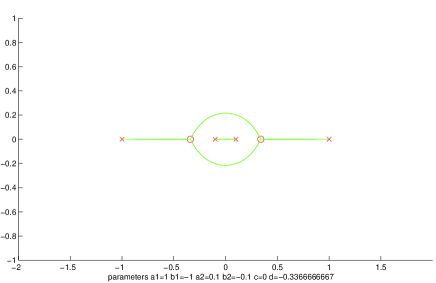
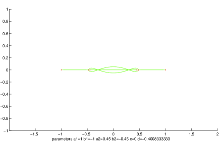
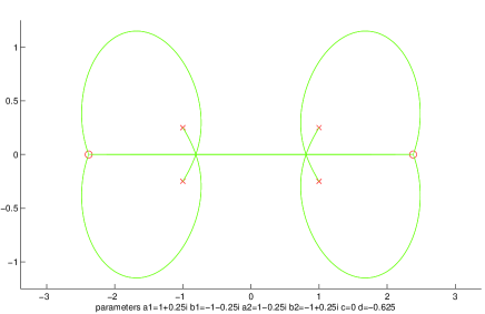
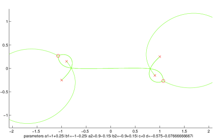
Figure 2.1: The set $\Gamma$ for $\mbox{genus }h=1$ and symmetric input $\{a_{1},b_{1},a_{2},b_{2}\}=\{a,-a,b,-b\}$.

Regarding the relation of $\Gamma$ and the Hermite-Padé polynomials for (1.5) we note the following. The first two examples for $\Gamma$ on Figure 2.1 correspond to the case when the intervals $(a_{j},b_{j})$, $j=1,2$ are one inside the other. In case when the intervals do not intersect (the so called Angelesco case), then $\mbox{genus }h=0$, see [8], [4]. The last two examples correspond to the case when these intervals are parallel and close to each other. If the distance between them increases, then again $\mbox{genus }h=0$, see [3].

2.2 “Optimization” procedure (genus $h=2$)

B. Beckermann suggested a numerical method to find the unknown parameters $(c,d)$ using a geometrical structure of the set $\Gamma$. The idea of the method is simple. You start from some approximate values $(\tilde{c},\tilde{d})$ for $(c,d)$ and from each branch point of the corresponding algebraic function $\tilde{h}$ you draw the elements of the set $\Gamma$, using the trajectories of the quadratic differentials. Then an optimization procedure is used to reach a coincidence of the corresponding trajectories which started from different branch points.

This numerical method works only for functions $h$ of genus 2, because these curves are in generic position among the curves defined by (1.9). The curves of lower genus are the result of algebraic degenerations and in order to find a numerical procedure for them we need to have their special parametrization.

In Figure 2.2 we have given examples of the set $\Gamma$ obtained by means of this method for the following input data (1.6):

1. $a_{1}=-2,b_{1}=1;a_{2}=-1,b_{2}=4;c=-0.2736665608,d=-1.689837898$.

2. $a_{1}=-5,b_{1}=1;a_{2}=1,b_{2}=5;c=0,d=-2.1647$.

In the first example (for $\vec{n}=(20,20)$ in (1.2)) we also plotted the zeros of the Hermite-Padé polynomials of type I ($\square$ and $\diamond$) and type II ($\ast$). Again the hard edges are indicated with a cross ($\times$) and the soft edges with a circle ($\circ$). The interesting parts of the picture have been blown up to show the details.

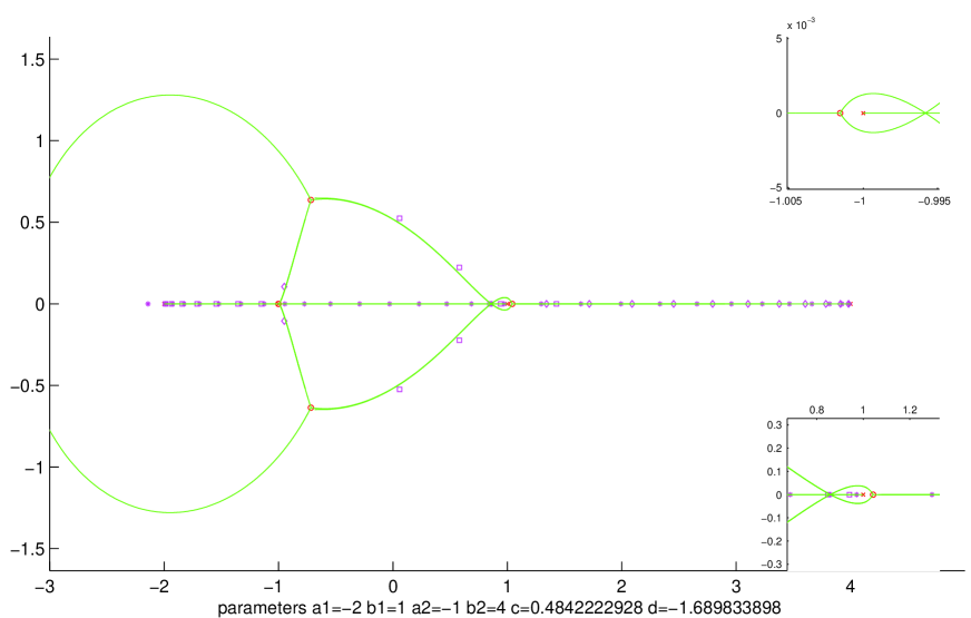
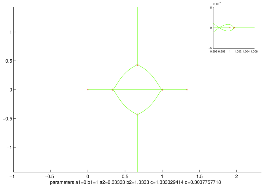
Figure 2.2: The set $\Gamma$ for the case genus $h=2$

Observe that H. Stahl (see [15], [16], [7]) has predicted $\Gamma$ (like in Figure 2.2) for the first time for Hermite-Padé polynomials for functions (1.5) with overlapping intervals $(a_{j},b_{j})$, $j=1,2$. Another case of overlapping intervals was considered in [6] and [12].

3 Hyperelliptic uniformization

Proof of Theorem 1.1. We are looking for a conformal map of the Riemann surface of $h$

$$h^{3}-3\frac{P_{2}(z)}{\Pi_{4}(z)}\,h+2\frac{P_{1}(z)}{\Pi_{4}(z)}=0\;,$$

on a hyperelliptic (two sheeted) Riemann surface (elliptic or ultra-elliptic, depending on the genus of $h$). Let $Q_{1}$ (of exact degree one) be the divisor in the Euclidean division of $P_{2}$ by $P_{1}$ with rest $Q_{0}$ of degree $0$, that is,

$$P_{2}-Q_{1}P_{1}=Q_{0},\quad\mbox{deg}\;Q_{0}=0.$$ (3.1)

Then we set

$$Q_{2}:=P_{1}Q_{1}^{3}-\Pi_{4}\,\Rightarrow\ \mbox{deg}\;Q_{2}\leqslant 2.$$

Indeed, if we substitute $P_{2}$ from (3.1) in (1.11), then due to (1.12) we have

$$\mbox{deg}\left((Q_{1}P_{1}+Q_{0})^{3}-\Pi_{4}P_{1}^{2}\right)=\mbox{deg}\left((Q_{2}P_{1}^{2}+3Q_{1}^{2}P_{1}^{2}Q_{0}+3Q_{1}P_{1}Q_{0}^{2}+Q_{0}^{3}\right)\leqslant 4.$$

The last inequality implies $\mbox{deg}(Q_{2}P_{1}^{2})\leqslant 4$ which proves $\mbox{deg}Q_{2}\leqslant 2$.

Next, we substitute the representation of $\Pi_{4}$ and $P_{2}$ by means of $Q_{2},Q_{1},Q_{0}$ and $P_{1}$ in the algebraic equation (1.9) for $h$

$$P_{1}Q_{1}^{3}h^{3}-Q_{2}h^{3}-3(P_{1}Q_{1}+Q_{0})h+2P_{1}=0,$$

and using the factorization $y^{3}+3y+2=(y-1)^{2}(y+2)$ for $y:=Q_{1}h$, we find

$$P_{1}(Q_{1}h-1)^{2}(Q_{1}h+2)-Q_{2}h^{3}-3Q_{0}h=0.$$

Now we introduce a new variable $w$ instead of $h$

$$w=\frac{1}{h}\,,$$

and we have

$$P_{1}(z)\,(Q_{1}(z)-w)^{2}(Q_{1}(z)+2w)-Q_{2}(z)-3Q_{0}w^{2}=0.$$

Then a new variable $R$ instead of $z$

$$R=z-w$$

transforms the third order equation into a quadratic equation

$$(P_{1}(R)+w)\,Q_{1}^{2}(R)\,(3w+Q_{1}(R))=Q_{2}(R+w)+3Q_{0}w^{2}.$$ (3.2)

We note that this magic drop in the degree of $w$ in (3.2) is in correspondence with the general fact [14] that any compact Riemann surface of genus less than or equal to 2 is conformally equivalent to a two sheeted hyper-elliptic Riemann surface, i.e., ultra-elliptic, elliptic or genus zero. This fact is not generally valid for genus greater than 2.

Then we substitute in (3.2) the expression

$$Q_{2}(R+w)=Q_{2}(R)+w\,Q_{2}^{\prime}(R)+\frac{w^{2}}{2}\,Q_{2}^{\prime\prime}(R)$$

where

$$Q_{2}=P_{1}Q_{1}^{3}-\Pi_{4}\,,\quad Q_{2}^{\prime}=Q_{1}^{3}+3P_{1}Q_{1}^{2}-\Pi_{4}\prime\,,\quad Q_{2}^{\prime\prime}=6Q_{1}^{2}+6P_{1}Q_{1}-\Pi_{4}^{\prime\prime}\,,$$

and after some cancelations we arrive at

$$\Pi_{4}(R)\,+\,\Pi^{\prime}_{4}(R)\,w\,+\,\left(\frac{\Pi_{4}^{\prime\prime}\,-\,3P_{2}}{2}\right)\,w^{2}\,=\,0.$$

From this we obtain

$$w=\frac{-\Pi^{\prime}_{4}(R)\pm\tilde{\Delta}(R)}{2K_{2}(R)},$$ (3.3)

where

$$\left\{\begin{array}[]{l}\tilde{\Delta}^{2}(R):=\left[\Pi^{\prime}_{4}(R)\right]^{2}-4\Pi_{4}(R)\,K_{2}(R),\\[20.0pt] K_{2}(R):=3R^{2}+2(c-s_{1})\,R-3d+s_{2},\end{array}\right.$$ (3.4)

We use (3.3) to define the new variable

$$\Delta=2K_{2}(R)w\,+\,\Pi_{4}^{\,\prime}(R).$$

Hence for each point $(z,h)$ of the Riemann surface $\mathfrak{R}$ we have a one to one correspondence with $(R,\Delta)$. If we fix just the value of $R$, then we have a two-valued function $\tilde{\Delta}(R)$ defined in (3.4).

For $h$ we have

$$h=-\frac{\Pi^{\prime}_{4}(R)\pm\tilde{\Delta}(R)}{2\Pi_{4}(R)}.$$ (3.5)

Thus we have obtained a hyperelliptic uniformization for the algebraic function of the third order $h(z)$

$$\left\{\begin{array}[]{l}h=-\displaystyle\frac{\Pi^{\prime}_{4}(R)\pm\tilde{\Delta}(R)}{2\Pi_{4}(R)}\,,\\[20.0pt] z=R+\displaystyle\frac{-\Pi^{\prime}_{4}(R)\pm\tilde{\Delta}(R)}{2K_{2}(R)}\,.\end{array}\right.$$ (3.6)

This proves the theorem. ∎

The Corollary 1.2 of Theorem 1.1 easily follows. Using (1.21) we have

$$\int h\,dz=\int h\,dR-\ln h,$$

and substituting (3.5) we arrive at (1.24). Another useful representation for the Abelian integral of Nuttall by means of elliptic integrals follows from

$$h\,dz=\left(\displaystyle\frac{\Pi_{4}^{\prime}(R)K^{\prime}_{2}(R)\,+\,4K^{2}_{2}(R)\,-\,2K_{2}(R)\Pi_{4}^{\prime\prime}(R)}{2K_{2}(R)\,\Delta}\,-\,\displaystyle\frac{K^{\prime}_{2}(R)}{2K_{2}(R)}\right)\,dR.$$ (3.7)

Now we consider an example of the conformal map (1.21) of the Riemann surface $\mathfrak{R}$ of the function $h$ of genus 1 with branch points $\{-1,-3/8,3/8,1\}$ on the two-sheeted Riemann surface $\mathfrak{H}(\Delta,R)$. Due to the symmetry we have (2.1), and then $d=-73/92$, $c=0$ and we can compute

$$\tilde{\Delta}^{2}=R^{2}\,\left(4R^{4}-\frac{73}{16}R^{2}+\frac{3601}{1024}\right),\qquad\Pi_{4}=R^{4}-\frac{73}{64}R^{2}+\frac{9}{64},\qquad K_{2}=2R^{2}.$$

The branch points of $\mathfrak{H}$ are

$$\tilde{\Delta}^{2}(R)=\prod_{j=1}^{4}(R-\epsilon_{j}),\qquad\epsilon_{j}=\pm\frac{\sqrt{146\pm 110i\sqrt{3}}}{16}.$$

Note that the images on $\mathfrak{H}$ of the branch points of $\mathfrak{R}$, containing the poles of $h$, have the same projections on the $R$-plane as their pre-images on the $z$-plane, i.e., in both cases the projections are $A_{1}\cup A_{2}$. In Figure 3.1 we illustrate this map, showing the images of the sheets of $\mathfrak{R}$ and some specific values of $h(z)$.

Figure 3.1: An example of the mapping of $\mathfrak{R}$ to $\mathfrak{H}$

4 Parametrization of $h$ of genus 1.

Proof of Theorem 1.3. We have to introduce a parameter $R_{0}$ and to find representations of $c(R_{0})$, $d(R_{0})$ for the coefficients of $P_{1}$, $P_{2}$ (see (1.13)), such that the algebraic condition (1.19), (1.13) to obtain genus 1 for the function $h$ is automatically fulfilled.

The dependence of the discriminant $\widetilde{D}(z)$ (see (1.11)) on $c$ and $d$ is rather complicated. However, the appearance of the parameters $c$ and $d$ in the discriminant $\Delta^{2}(R)$ (see (3.4)) is linear. This easily allows us to choose for the parameter $R_{0}$ the double zero of $\Delta^{2}(R)$ (which characterizes the case of genus 1 for $h$) to find representations for $c(R_{0})$ and $d(R_{0})$.

We denote

$$c_{1}=2(c-s_{1}),\quad c_{2}=s_{2}-3d.$$ (4.1)

Therefore, due to (3.4),

$$\Delta^{2}(R):=\left[\Pi^{\prime}_{4}(R)\right]^{2}-4\Pi_{4}(R)\,K_{2}(R)\;,\quad K_{2}(R)=3R^{2}+c_{1}R+c_{2}\;,$$

and the condition on $R_{0}$ to be a double zero of $\Delta^{2}(R)$ is

$$\quad\left\{\begin{array}[]{l}\Delta^{2}(R_{0})=0,\\[20.0pt] \displaystyle\frac{d}{dR}\,\,\Delta^{2}(R)\Bigl{|}_{R=R_{0}}=0,\\ \end{array}\right.$$ (4.2)

which is a linear system of equations for the determination of the parameters $c_{1}$ and $c_{2}$ (and therefore $c,d$ as well). The solution of (4.2) is

$$c_{1} = \frac{1}{16\Pi_{4}^{2}(R_{0})}\left(8\Pi_{4}(R_{0})\,\Pi^{\prime}_{4}(R_{0})\,\Pi^{\prime\prime}_{4}(R_{0})-96R_{0}\Pi_{4}^{2}(R_{0})-4\Pi_{4}^{{}^{\prime}3}(R_{0})\right),$$

$$c_{2} = \frac{1}{16\Pi_{4}^{2}(R_{0})}\Bigl{(}-8\,R_{0}\Pi_{4}(R_{0})\,\Pi^{\prime}_{4}(R_{0})\,\Pi^{\prime\prime}_{4}(R_{0})+48R_{0}^{2}\Pi_{4}^{2}(R_{0})$$

$$+\ 4\Pi_{4}^{{}^{\prime}3}(R_{0})\,R_{0}+4\Pi_{4}^{{}^{\prime}2}(R_{0})\,\Pi_{4}(R_{0})\Bigr{)}.$$

In this way we have a representation for $K_{2}(R)$ in (3.4)

$$K_{2}(R)=\frac{1}{4\Pi_{4}^{2}(R_{0})}\Bigl{[}12(R-R_{0})^{2}\Pi_{4}^{2}(R_{0})\\ +\ (R-R_{0})\bigl{(}2\Pi_{4}(R_{0})\Pi^{\prime}_{4}(R_{0})\,\Pi^{\prime\prime}_{4}(R_{0})+\Pi_{4}^{{}^{\prime}3}(R_{0})\bigr{)}+\Pi_{4}(R_{0})\,\Pi_{4}^{{}^{\prime}2}(R_{0})\Bigr{]}.$$ (4.4)

Finally, adding the useful expressions (see (3.4) and (1.13)):

$$P_{2}(z) = \frac{1}{6}\Pi^{\prime\prime}_{4}(z)-\frac{1}{3}K_{2}(z)$$

$$P_{1}(z) = \frac{1}{6}\Pi^{\prime\prime\prime}_{4}(z)-\frac{1}{2}K^{\prime}_{2}(z),$$ (4.5)

we obtain the parametrization of the algebraic curve $h$ (see (1.13)) of genus 1 by the parameter $R_{0}$, by means of (1.9),  (4.4) and (4). This proves the theorem. ∎

5 An example of the determination of $h$ of genus 1

We present an application of the $R_{0}$-parametrization in order to determine the unknown parameters of the algebraic function (1.9), (1.13) of genus 1 for nonsymmetric input data $\{a_{1},b_{1},a_{2},b_{2}\}$.

We consider the integral along the closed contour $\mathfrak{L}\subset\mathfrak{R}$

$$I:=\int\limits_{\mathfrak{L}}\,h(\dot{z})\,d\pi(\dot{z}).$$ (5.1)

This contour (see Figure 3.1) starts at the point $\infty^{(0)}$, goes along the pre-image of the negative part of the real axis on $\mathfrak{R}_{0}$ up to the branch point $a_{1}$, where it lifts to $\mathfrak{R}_{1}$ and continues in the reverse direction along the pre-image of the real axis via the point $\infty^{(1)}$ up to the branch point $b_{1}$ where it returns to $\mathfrak{R}_{0}$ and continues in the reverse direction along the pre-image of the real axis up to the point $\infty^{(0)}$. Then we slightly deform $\mathfrak{L}$ so that the new contour $\widetilde{\mathfrak{L}}$ does not contain the pre-images of the real axes and infinity points from the corresponding sheets of $\mathfrak{R}$. This deformation does not change the value of $I$.

We fix the parameter $R_{0}$ and substitute (4.4) in (1.24), we apply (1.24) to the integral (5.1) along $\widetilde{\mathfrak{L}}$ and we note that the periods of the outside integral terms are purely imaginary and therefore

$$\mathop{\textrm{missing}}{Re}I=\mathop{\textrm{missing}}{Re}\int\limits_{\widetilde{\mathfrak{M}}}\displaystyle\frac{\Delta(\dot{R})\,d\pi(\dot{R})}{2\Pi_{4}(\dot{R})}\,.$$ (5.2)

Here the contour $\widetilde{\mathfrak{M}}\subset\mathfrak{H}$ is the image of the contour $\widetilde{\mathfrak{L}}\subset\mathfrak{R}$. We introduce the notation

$$J(R):=-\displaystyle\frac{\Delta(R)\,dR}{2\Pi_{4}(R)},\quad\Delta(R):=\left(R-R_{0}\right)\,\sqrt{\left(\displaystyle\frac{\Pi^{\prime}_{4}(R)^{2}-4\Pi_{4}\,K_{2}}{(R-R_{0})^{2}}\right)},$$

where the continuous branch of the square root is used for which $\sqrt{x}>0\,,\,\,\,x\rightarrow\infty$. In this notation the integral (5.2) can be written in the form

$$\mathop{\textrm{missing}}{Re}I=\mathop{\textrm{missing}}{Re}\int\limits_{\pi(\widetilde{\mathfrak{M}})}J(R)\,dR\,.$$

If we deform $\widetilde{\mathfrak{M}}$ to the contour $\mathfrak{M}\subset\mathfrak{H}$ which is the image of the contour $\mathfrak{L}\subset\mathfrak{R}$ (note that $\pi(\mathfrak{M})=\mathbb{R}\subset\bar{\mathbb{C}}$ ), then the function in the integrand of (5.2) has singularities at the point $\dot{\infty}\in\mathfrak{M}$ and at the images of the branch points $\{a_{j},\,b_{j}\}$ on $\mathfrak{M}$. The following behavior holds near infinity and near the branch points

$$J(R)\sim-\frac{1}{R},\quad R\rightarrow\infty,\qquad J(R)\sim\frac{(-1)^{j}}{2(R-a)},\quad R\rightarrow a\in\{a_{j},\,b_{j}\}.$$

Taking the regularization function

$$\mbox{Reg}(R):=\frac{1}{2(R-a_{2})}+\frac{1}{2(R-b_{2})}-\frac{1}{2(R-a_{1})}-\frac{1}{2(R-b_{1})}-\frac{R}{2(R^{2}+1)},$$

we have

$$\mathop{\textrm{missing}}{Re}\int\limits_{\pi(\widetilde{\mathfrak{M}})}\mbox{Reg}(R)\,\,dR=0.$$

Thus, we obtain a formula which we can use for the numeric computation of the real part of the Nuttall’s Abel integral

$$\mathop{\textrm{missing}}{Re}I\,=\,\mathop{\textrm{missing}}{Re}\int\limits_{-\infty}^{\infty}(\,J(R)\,-\,\mbox{Reg}(R)\,)\,dR.$$

Now, in accordance with (1.16), (1.18) we choose $R_{0}$ such that $\mathop{\textrm{missing}}{Re}I=0$.

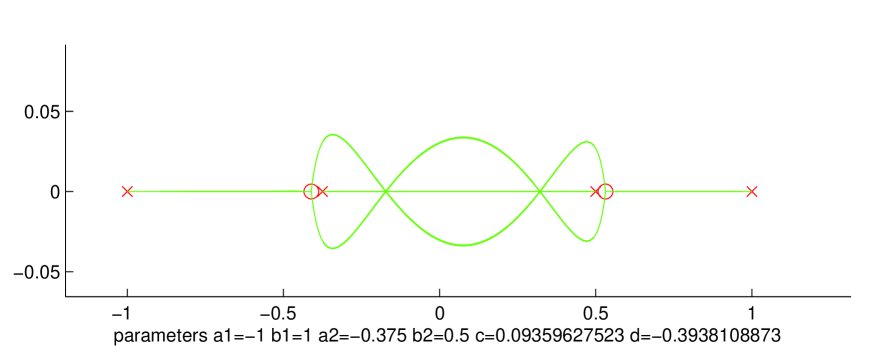
Figure 5.1: $\Gamma$ for genus h = 1 and symmetric input $\{a_{1},b_{1},a_{2},b_{2}\}=\{-1,-3/8,1/2,1\}$.

For the input data $a_{1}=-1$, $b_{1}=1$, $a_{2}=-3/8$, $b_{2}=4/8$, this procedure gives

$$R_{0}=0.0775\quad\Rightarrow\quad\mathop{\textrm{missing}}{Re}I=0.001,\qquad R_{0}=0.0774\quad\Rightarrow\quad\mathop{\textrm{missing}}{Re}I=-0.0006.$$

An independent verification of this procedure can be done by using the Beckermann method from Subsection 2.2, see Figure 5.1 for $R_{0}=0.0775$.

References

- [1] A. I. Aptekarev, Multiple orthogonal polynomials, J. Comput. Appl. Math. 99 (1998), no. 1–2, 423–447.
- [2] A. I. Aptekarev, Asymptotics of Hermite-Padé approximants for two functions with branch points, Dokl. Math. 78 (2), (2008), 717–719.
- [3] A. I. Aptekarev, V. A. Kalyagin , V. G. Lysov and D. N. Toulyakov, Equilibrium of vector potentials and uniformization of the algebraic curves of genus 0, J. Comput. Appl. Math. 233 (2), (2009), 602–616.
- [4] A. I. Aptekarev, A. B. J. Kuijlaars and W. Van Assche, Asymptotics of Hermite-Padé rational approximants for two analytic functions with separated pairs of branch points (case of genus 0), International Mathematics Research Papers, 2008 (2008) , Article ID rpm007, 128 pages.
- [5] A. I. Aptekarev, V. G. Lysov and D. N. Toulyakov, Three-sheeted Riemann surfaces of genus 0 with fixed projections of the branch points, Preprint, Inst. Appl. Math. Russia Akad. Sci. (13) (2007), (in Russian, http://www.keldysh.ru/papers/2007/source/prep200713.pdf)
- [6] A.I. Aptekarev, V.G. Lysov, Systems of Markov functions generated by graphs and the asymptotics of their Hermite-Padé approximants, Mat. Sb. (201 (2010), no. 2, 29–78 (in Russian); translated in Sb. Math. 201 (2010), no. 1–2, 183–234.
- [7] A. I. Aptekarev and H. Stahl, Asymptotics of Hermite-Padé polynomials, in Progress in Approximation Theory (A. Gonchar, E. B. Saff, eds.), Springer-Verlag, Berlin, 1992, pp. 127–167.
- [8] A. A. Gonchar and E. A. Rakhmanov, On the convergence of simultaneous Padé approximants for systems of functions of Markov type, Trudy Mat. Inst. Steklov. 157 (1981), 31–48 (in Russian); translated in Proc. Steklov Inst. Math. 157 (1983), 31–50.
- [9] C. Hermite, Sur la fonction exponentielle, C.R. Acad. Sci. Paris 77 (1873), 18–24; 74–79; 226–233.
- [10] G. López Lagomasino, D. Pestana, J. M. Rodríguez, D. Yakubovich, Computation of conformal representations of compact Riemann surfaces, Math. Comp. 79 (2010), 365–382.
- [11] J. Nuttall, Asymptotics of diagonal Hermite-Padé polynomials, J. Approx. Theory 42 (1984), no. 4, 299–386.
- [12] E. A. Rakhmanov, The asymptotics of Hermite-Padé polynomials for two Markov-type functions, Mat. Sb. 202 (2011), no. 1, 133–140 (in Russian); translated in Sb. Math. 202 (2011), no. 1–2, 127–134.
- [13] E. A. Rakhmanov and S. P. Suetin, The distribution of the zeros of the Hermite-Padé polynomials for a pair of functions forming a Nikishin system, Mat. Sb. 204 (2013), no. 9, 115–160 (in Russian); translated in Sb. Math. 204 (2013), no. 9–10, 1347–1390.
- [14] C. L. Siegel, Topics in Complex Function Theory, Volume 2, Automorphic Functions and Abelian Integrals, Wiley-Interscience, New York, 1973.
- [15] H. Stahl, Asymptotics of Hermite-Padé polynomials and related convergence results — a summary of results, Nonlinear numerical methods and rational approximation (Wilrijk, 1987), Math. Appl., 43, Reidel, Dordrecht, 1988, 23–53.
- [16] H. Stahl, Asymptotics of Hermite-Padé polynomials and related approximants. A summary of results, (unpublished, 79 pages).
- [17] W. Van Assche, Multiple orthogonal polynomials, irrationality and transcendence, in “Continued fractions: from analytic number theory to constructive approximation”, Contemporary Mathematics 236 (1999), 325–342.