Stabilization of solitons under competing nonlinearities by external potentials

Abstract

We report results of the analysis for families of one-dimensional (1D) trapped solitons, created by competing self-focusing (SF) quintic and self-defocusing (SDF) cubic nonlinear terms. Two trapping potentials are considered, the harmonic-oscillator (HO) and delta-functional ones. The models apply to optical solitons in colloidal waveguides and other photonic media, and to matter-wave solitons in Bose-Einstein condensates (BEC) loaded into a quasi-1D trap. For the HO potential, the results are obtained in an approximate form, using the variational and Thomas-Fermi approximations (VA and TFA), and in a full numerical form, including the ground state and the first antisymmetric excited one. For the delta-functional attractive potential, the results are produced in a fully analytical form, and verified by means of numerical methods. Both exponentially localized solitons and weakly localized trapped modes are found for the delta-functional potential. The most essential conclusions concern the applicability of competing Vakhitov-Kolokolov (VK) and anti-VK criteria to the identification of the stability of solitons created under the action of the competing SF and SDF terms.

Solitons, i.e., nondiffracting beams propagating in nonlinear media, are formed thanks to an interplay between diffraction, which tends to spread the beam, and the self-induced change of the nonlinear refractive index of the medium. Optical solitons are important for their capability to beat diffraction, and their potential for engineering a variety of reconfigurable optical structures including (and not limited to) couplers, deflectors, and logic gates. A classical example of the setting supporting solitons is provided by Kerr media, featuring the third-order self-focusing nonlinearity. However, more complex optical media (for instance, colloids filled by metallic nanoparticles) often exhibit competing nonlinearities of different orders, most typically self-focusing cubic and self-defocusing quintic. In the latter case, stable optical solitons also propagate through the medium, differing from the Kerr solitons by a broader shape. More challenging is the opposite case of the competition between the lower-order (cubic) self-defocusing and higher-order (quintic) self-focusing nonlinearities. In the uniform medium, this combination may generate only strongly unstable solitons. In this work we demonstrate that the latter situation can be remedied by an effective trapping potential. In term of optical media, the potential represents a waveguiding structure, and, by itself, it is a linear ingredient of the system. We predict that trapping potentials, both tight and loose, readily stabilize vast families of solitons, which are completely unstable in the uniform medium.

I Introduction

Competition between self-focusing (SF) and self-defocusing (SDF) nonlinearities occurs in various physical media, playing an important role in the creation of self-trapped modes (in particular, solitons). A well-known example is the competition between quadratic (second-harmonic-generating, alias $\chi^{(2)}$) and SDF cubic nonlinear interactions in optics, in the case when the proper choice of the mismatch constant makes the $\chi^{(2)}$ interaction effectively self-focusing Trillo and Wabnitz (1992); Karpierz (1995); Trillo, Buryak, and Kivshar (1996); Bang, Kivshar, and Buryak (1997); Bang et al. (1998); Alexander et al. (2000); Towers et al. (2001); Etrich et al. (2000); Buryak et al. (2002).

A large number of publications have addressed systems featuring the competition between SF cubic and SDF quintic terms. Such combinations of nonlinear terms frequently occur in optics, including liquid waveguides Zhan et al. (2002); Ganeev et al. (2004); Falcao-Filho et al. (2013), special kinds of glasses Zhan et al. (2002); Boudebs et al. (2003); Ogusu et al. (2004); Sanchez et al. (2004) and ferroelectric films Gu et al. (2009). Especially flexible are colloidal media formed by metallic nanoparticles, in which the cubic-quintic (CQ) optical nonlinearity can be adjusted within broad limits by selecting the size of the particles and the colloidal filling factor Falcao-Filho, de Araújo, and Rodrigues (2007); Falcao-Filho et al. (2010); Garcia et al. (2012); Reyna and de Araújo (2014).

The SF-SDF CQ nonlinearity has a great potential for the creation of stable multidimensional solitons, including two- Quiroga-Teixeiro and Michinel (1997); Quiroga-Teixeiro, Berntson, and Michinel (1999); Pego and Warchall (2002); Crasovan, Malomed, and Mihalache (2001) and three- Mihalache et al. (2002, 2004) dimensional (2D and 3D) solitary vortices, as reviewed in Ref. Malomed et al. (2005) and recently demonstrated experimentally in the 2D setting, in the colloidal waveguide, in Ref. Falcao-Filho et al. (2013). Indeed, the cubic-only SF nonlinearity cannot create stable multidimensional solitons, as the corresponding 2D self-trapped modes (alias Townes’ solitons) and 3D solitons are subject to instabilities related to the critical collapse in 2D [recently, it was demonstrated that stable 2D composite (half-fundamental - half-vortical) solitons can be created in a two-component system combining the cubic self-attraction and linear mixing of the components through first-order spatial derivatives, which represent the spin-orbit couplingSakaguchi, Li, and Malomed (2014)], and supercritical collapse in 3D Bergé (1998); Kuznetsov and Dias (2011)(spatial inhomogeneity, in the form of a finite jump of the SF Kerr coefficient between an inner circle and the surrounding area, may stabilize fundamental solitons Sakaguchi and Malomed (2012)). The additional SDF quintic term arrests the collapse, imposing soliton stability Quiroga-Teixeiro and Michinel (1997); Quiroga-Teixeiro, Berntson, and Michinel (1999); Pego and Warchall (2002); Crasovan, Malomed, and Mihalache (2001); Malomed et al. (2005); Mihalache et al. (2002, 2004).

The study of the competing CQ nonlinearities is also relevant in 1D settings. A remarkable fact is that, although the 1D nonlinear Schrödinger (NLS) equation with the combined CQ nonlinearity is not integrable, it admits well-known exact solutions for the full soliton family Pushkarov, Pushkarov, and Tomov (1979); Cowan et al. (1986). Furthermore, these solitons are stable not only in the case of the competition between the SF cubic and SDF quintic terms, but also when both terms have the SF sign Pelinovsky, Kivshar, and Afanasjev (1998). The latter fact is surprising, because the 1D solitons created by the quintic-only SF term are, as a matter of fact, a 1D version of the Townes’ solitons Gaididei, Schjodt-Eriksen, and Christiansen (1999); Abdullaev and Salerno (2005); Alfimov, Konotop, and Pacciani (2007), and, accordingly, are unstable against the 1D variety of the critical collapse. When both cubic and quintic SF terms are present, the 1D solitons may still be pushed into the collapse by strong perturbations (sudden compression), but, somewhat counter-intuitively, they are stable against small perturbations.

In the case of the combination of the SDF cubic and SF quintic terms, the entire family of 1D solitons is completely unstable. We stress that this combination of the competing nonlinearities may be physically relevant. In addition to the optical examples mentioned above, it appears naturally as a result of the reduction of the 3D Gross-Pitaevskii (GP) equation to the 1D form for cigar-shaped traps filled with atomic Bose-Einstein condensates (BECs) Muryshev et al. (2002); Salasnich, Parola, and Reatto (2002a, b); Carr and Brand (2004a, b); Khaykovich and Malomed (2006). In the latter case, the sign of the cubic terms is determined by the sign of the scattering length in the BEC, and typically corresponds to the SDF, while the quintic term is generated by the tight confinement of the condensate in the transverse plane, and always corresponds to the SF.

Thus, search for physically realistic settings that would allow the stabilization of 1D solitons in the NLS equation with the SDF-SF combination of the cubic and quintic terms is an interesting problem, which is the subject of the present work. It is well known that 2D Townes solitons and solitary vortices, created by the SF cubic nonlinearity, can be readily stabilized by an harmonic-oscillator (OH) trapping potential Dalfovo and Stringari (1996); Dodd (1996); Alexander and Bergé (2002); Mihalache et al. (2006); Carr and Clark (2006), or by periodic potentials provided by optical lattices Baizakov, Malomed, and Salerno (2003); Yang and Musslimani (2003). In this work, we consider the stabilization of 1D solitons provided by the HO potential, and also by the delta-functional attractive potential. In the optical waveguide, effective traps may be induced by a transverse profile of the refractive index Kivshar and Agrawal (2003), while in the BEC setup traps are created by means of properly tailored magnetic and/or optical fields Giorgini, Pitaevskii, and Stringari (2008); Strecker et al. (2003). In these contexts, both broad HO traps and narrow ones, which may be approximated by the Dirac’s delta-function, are in principle relevant settings.

The NLS equation with the SDF-SF CQ nonlinearity and a trapping potential offers a possibility to explore peculiarities of the stabilization of 1D solitons under the action of the competing nonlinear terms, which is especially interesting as concerns the central issue of this topic, i.e., identification of the stability of the so produced solitons. Indeed, it is commonly known that the necessary stability criterion for families of solitons supported by the SF nonlinearity is provided by the Vakhitov- Kolokolov (VK) criterion Vakhitov and Kolokolov (1973); Bergé (1998); Kuznetsov and Dias (2011), which is simply formulated in terms of the dependence between the soliton’s norm (total power), $N$, and its propagation constant, $k$: $dN/dk>0$. In some cases, this stability criterion may actually be a sufficient one, too. On the other hand, for solitons supported by the interplay of SDF nonlinearity and trapping potentials, a necessary stability condition is provided by the anti-VK criterion, $dN/dk<0$ Sakaguchi and Malomed (2010). Therefore, a natural question, which we address in the present work, is what criterion determines the stability of solitons in the case of the competition between the SDF cubic and SF quintic terms. In the opposite case of the combination of the SF cubic and SDF quintic nonlinearities, the former one dominates the formation of 1D solitons, their entire family being stable in accordance with the VK criterion.

The rest of the paper is organized as follows. The model is formulated in Section II. Findings for the soliton trapped in the HO potential are collected in Section III, which includes both approximate analytical results, obtained by means of the variational and Thomas-Fermi approximations (VA and TFA correspondingly), and systematically generated numerical results for the existence and stability of the solitons. A significant conclusion is that the usual VK criterion works, as the necessary and sufficient one, for forward-going branches of $N(k)$ curves of soliton families, in either case of the positive and negative local slope ($dN/dk\gtrless 0$), while the anti-VK criterion works equally well, but for backward-going branches. Both these types of branches are produced by the analytical and numerical results under the action of the HO trap. Findings for the delta-functional potential are reported in Section IV, including both exponentially localized solitons and weakly localized but normalizable trapped modes. In fact, they are obtained in a fully analytical form, which is verified by dint of the numerical analysis, and it is again demonstrated that the usual VK criterion is correct for all the solitons in the case of forward-going branches, while the anti-VK is proper for backward-going ones. The paper is concluded by Section V.

II The model

In the free space, the 1D NLS equation with the SDF cubic and SF quintic terms is

$$i\frac{\partial u}{\partial z}+\frac{1}{2}\frac{\partial^{2}u}{\partial x^{2}}-g|u|^{2}u+|u|^{4}u=0,$$ (1)

where $g\geq 0$ is the strength of the cubic nonlinearity. Here, Eq. (1) is written in the form of the paraxial equation for the spatial evolution of the optical beam in a nonlinear planar waveguide, $z$ and $x$ being the longitudinal and transverse coordinates, respectively Kivshar and Agrawal (2003). In physical units, the solitons considered below may have the transverse width $\lesssim 50$ $\mathrm{\mu}$m, while the experimentally relevant transmission distance may be a few cm. If Eq. (1) is considered as the reduced GP equation for the BEC, the solitons may be composed of several thousands of atoms, with the characteristic size $\lesssim 100$ $\mathrm{\mu}$m Strecker et al. (2003).

Equation (1) has a family of exact soliton solutions with propagation constant $k\geq 0$, which can be easily obtained from the well-known solitons for the opposite case of the SF-SDF CQ nonlinearity Pushkarov, Pushkarov, and Tomov (1979) by means of the analytical continuation:

$$u\left(x,z\right)=e^{ikz}\sqrt{\frac{2\sqrt{3}k}{\sqrt{4k+3g^{2}/4}\cosh\left({2\sqrt{2k}x}\right)-(g/2)\sqrt{3}}}$$ (2)

(in the case of the GP equation, $-k$ is the chemical potential of the BEC). The norm of the soliton (2), which represents the total power of the spatial optical solitons, or the total number of atoms in matter-wave solitons in BEC, is

$$N(k)\equiv\int_{-\infty}^{+\infty}|u(x)|^{2}dx=\sqrt{6}\arctan\left({\frac{2\sqrt{k}}{\sqrt{4k+3g^{2}/4}-(g/2)\sqrt{3}}}\right).$$ (3)

This soliton family is completely unstable. Notice that $N(k)$, as given by Eq. (3) yields $dN/dk<0$, hence it does not satisfy the VK criterion Vakhitov and Kolokolov (1973).

As said above, solitons can be stabilized by means of an external potential, $W(x)$, which added to Eq. (1) gives:

$$i\frac{\partial u}{\partial z}+\frac{1}{2}\frac{\partial^{2}u}{\partial x^{2}}-g|u|^{2}u+|u|^{4}u=W(x)u.$$ (4)

The stationary version of Eq. (4), corresponding to $u\left(x,z\right)=\exp\left(ikz\right)U(x)$, is

$$-kU+\frac{1}{2}U^{\prime\prime}-gU^{3}+U^{5}=W(x)U.$$ (5)

In the optical waveguide, the potential represents an inhomogeneous profile of the refractive index, while in the BEC trap it may be induced by an external laser beam. In either type of the physical situation imposed potential may be either broad (width measured by dozens of $\mathrm{\mu}$m) or narrow o(squeezed to a few $\mathrm{\mu}$m). Here we consider two basic types of the trapping potential, harmonic trap,

$$W(x)=({1/2})\Omega^{2}x^{2},$$ (6)

and the Dirac’s delta-function,

$$W(x)=-\epsilon\delta(x)$$ (7)

with $\epsilon>0$. By the means of rescaling, we fix $\Omega\equiv 0.5$ in Eq. (6), and $\epsilon=0.5$ in Eq. (7).

The delta-functional attractive potential (7) implies that the $x$-derivative of the wave field is a subject to a jump condition at $x=0$:

$$u_{x}\left(x=+0\right)-u_{x}\left(x=-0\right)=-2\epsilon u(x=0),$$ (8)

while the field itself is continuous at this point. In fact, a full family of solitons pinned to the ideal delta-functional potential embedded into the medium with the CQ nonlinearity can be found in an exact analytical form, as shown below in Section IV.

III The harmonic-oscillator potential

In this section we present results obtained for Eq. (5) with the HO potential (6). We first use analytical approximations to gain a first insight as to where one may expect solitons, and then we concentrate on numerical analysis in these regions.

III.1 The variational approximation (VA)

The stationary NLSE equation is now given by

$$-kU+\frac{1}{2}U^{\prime\prime}-gU^{3}+U^{5}=\frac{1}{2}\Omega^{2}x^{2}U,$$ (9)

where $k$ is the propagation constant, the prime stands for $d/dx$, and the HO potential is introduced as per Eq. (6). The starting point of the VA is that Eq. (9) can be derived from the Lagrangian density,

$$2\mathcal{L}=\frac{1}{2}\left(U^{\prime}\right)^{2}+kU^{2}+\frac{1}{2}gU^{4}-\frac{1}{3}U^{6}+\frac{1}{2}\Omega^{2}x^{2}U^{2}.$$ (10)

We approximate the fundamental trapped mode by the usual Gaussian ansatz Anderson (1983); Malomed (2002),

$$u(x)=A\exp\left(-x^{2}/w^{2}\right),$$ (11)

with amplitude $A$, width $w$, and norm

$$N_{\mathrm{VA}}=\sqrt{\pi/2}A^{2}w.$$ (12)

The substitution of ansatz (11) into Eq. (10) and integration over $x$ yields the corresponding effective Lagrangian, $L=\int_{-\infty}^{+\infty}\mathcal{L}(x)dx$,

$$\frac{2L}{\sqrt{\pi}}=\frac{1}{2}\left(\frac{2}{w^{4}}+\frac{1}{2}\Omega^{2}\right)A^{2}\left(\frac{w}{\sqrt{2}}\right)^{3}+\frac{w}{\sqrt{2}}kA^{2}+\frac{1}{4}gA^{4}w-\frac{1}{3}A^{6}\frac{w}{\sqrt{6}},$$ (13)

which gives rise to the respective Euler-Lagrange equations, $\partial L/\partial A^{2}=\partial L/\partial w=0$, i.e.,

$$\frac{1}{2}\left(\frac{2}{w^{4}}+\frac{1}{2}\Omega^{2}\right)\left(\frac{w}{\sqrt{2}}\right)^{3}+\frac{kw}{\sqrt{2}}+\frac{1}{2}gA^{2}w-A^{4}\frac{w}{\sqrt{6}}=0,$$ (14)

$$-\frac{1}{w^{2}\sqrt{2}}+\frac{3}{4}\Omega^{2}\frac{w^{2}}{(\sqrt{2})^{3}}+\frac{k}{\sqrt{2}}+\frac{1}{4}gA^{2}-\frac{1}{3}\frac{A^{4}}{\sqrt{6}}=0.$$ (15)

Equation (15) produces two solutions for the squared amplitude,

$$A_{\pm}^{2}=\sqrt{\frac{3}{8}}g\pm\sqrt{\frac{3}{8}g^{2}+\frac{\sqrt{3}}{4}\left(\frac{2}{w^{2}}+\frac{1}{2}\Omega^{2}w^{2}+4k\right)}.$$ (16)

Solution $A_{+}^{2}$ is physical (positive) under condition $k\geq-\frac{\sqrt{3}}{8}g^{2}-\frac{1}{2}w^{-2}-\frac{1}{8}\Omega^{2}w^{2}$, while $A_{-}^{2}$ is relevant only for $-\frac{\sqrt{3}}{8}g^{2}-\frac{1}{2}w^{-2}-\frac{1}{8}\Omega^{2}w^{2}\leq k<-\frac{1}{2}w^{-2}-\frac{1}{8}\Omega^{2}w^{2}$. In Fig. (1) a typical fundamental-mode profile produced by the VA is compared to its numerical counterpart.

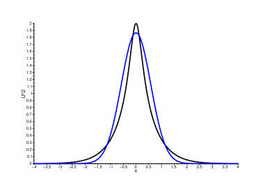
Figure 1: The wave function of the fundamental mode trapped in the HO potential (6) with $\Omega=0.5$, as obtained in the numerical form, by means of the shooting method (the black, taller profile), and as predicted analytically by the VA (the blue, lower profile) for $g=2$, $k=1.309$, $N=2.69$. The norm is calculated for the numerical solution.

III.2 The Thomas-Fermi approximation (TFA)

For negative values of $k$ in Eq. (9), another analytical approach may be applied, in the form of the TFA, which neglects the diffraction term, $d^{2}U/dx^{2}$, in the equation. This approximation, which is relevant for confined modes when the SDF nonlinear term is the dominant one Borovkova et al. (2011a, b), yields the stationary solution in the form of

$$U_{\mathrm{TFA}}^{2}(x)=\left\{\begin{array}[]{c}\frac{g}{2}-\sqrt{\frac{g^{2}}{4}-\left(|k|-\frac{1}{2}\Omega^{2}x^{2}\right)},~{}\mathrm{at}~{}~{}x^{2}<2|k|/\Omega^{2},\\ 0,~{}\mathrm{at}~{}~{}x^{2}>2|k|/\Omega^{2}.\end{array}\right.$$ (17)

As seen from Eq. (17), the TFA solution is a physically relevant provided that the wavenumber satisfies condition $0<-k<g^{2}/4$. There exists also a solution with the positive sign in front of the square root in Eq. (17), but it is irrelevant, as it does not vanish at $|x|\rightarrow\infty$. The comparison of typical solution profiles predicted by the TFA with their numerical counterparts is presented in Fig. 2. It can be concluded that the TFA predicts the solutions in a qualitatively correct form only when the cubic SDF term dominates in Eq. (9), which occurs at $g\gtrsim 2$.

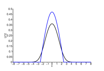
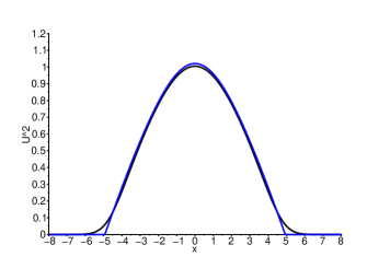
Figure 2: Examples of the fundamental mode trapped in the HO potential, as obtained in the numerical form (the black, lower profiles), and by means of the TFA (the blue profiles with truncated tails), for $g=2,k=-0.72,N=1.17$ (a) and $g=4,k=-3.041,N=6.15$ (b).

III.3 Numerical results

III.3.1 Fundamental solutions

Numerical stationary solutions for HO potential were found by means of the imaginary-time-integration Chiofalo, Succi, and Tosi (2000) and shooting Bridges, Derks, and Gottwald (2002) methods. The results are collected in Fig. 3, where the corresponding dependences $N(k)$ are displayed for different values of the cubic-SDF coefficient, $g$, and compared to the results produced by the VA and TFA. All the branches stem, at $N=0$, from the point which corresponds to the fundamental mode of the HO potential in linear quantum mechanics.

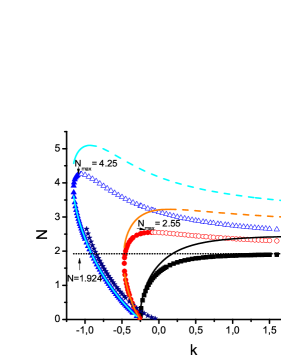
Figure 3: The norm of the fundamental modes, trapped in the HO potential (6) versus $k$ for different values of $g$. Here and in Fig. 5 below, full and empty marks designate, respectively, stable and unstable solutions found numerically: black (squares) for $g=0$, red (circles) for $g=1$, and blue (triangles) for $g=2$. Solid and dashed lines depict VK-stable and unstable states predicted by the VA: black (the lowest line in the graph) for $g=0$, orange (the middle one) for $g=1$ and cyan (the highest position in the graph) for $g=2$. Results obtained for $g=2$ by the means of TFA are depicted by navy-blue stars. The black dotted horizontal line here and in Fig. 5 corresponds to the limit value of $N(k=\infty)=(\sqrt{6}/4)\pi\approx 1.924$, see Eq. (3), which does not depend on $g$. Higher order modes are not included here.

The maximum value of dependence $N(k)$ increases with the growth of $g$. The turning point, where the two branches of the VA solution meet, can be estimated from Fig. 3. For instance, it is $k\approx-1$ at $g=2$. Only a small part of the top (blue) solution branch in Fig. 3 satisfies the Vakhitov-Kolokolov (VK) criterion, $dN/dk>0$, which, as said above, is a necessary condition for the stability of localized modes supported by the SF nonlinearity Vakhitov and Kolokolov (1973). On the other hand, the necessary stability condition for localized modes dominated by the SDF nonlinearity may switch from the VK form to the anti-VK one, $dN/dk<0$ Sakaguchi and Malomed (2010). Because the present model features the competition of the quintic SF and cubic SDF terms, it is not obvious which one plays the dominant role at different values of $k$ and $N$, hence a numerical stability analysis is necessary.

To explore the stability of the solutions, eigenfrequencies of small perturbations around the stationary solutions have been computed, using the standard linearization procedure Yang (2010). For stable solutions, imaginary parts of these frequencies are zero (or negligibly small, in terms of the numerical computation). All instabilities detected by this method feature pure-imaginary eigenvalues (i.e., the respective instability mode is expected to grow exponentially without oscillations). The latter finding suggests that the VA and anti-VK criteria may be sufficient for the stability analysis, because what they cannot detect, are complex unstable eigenvalues Vakhitov and Kolokolov (1973); Bergé (1998), which do not exists in the present setting anyway. Eventually, the full results for the (in)stability eigenvalues demonstrate that the VA criterion correctly predicts the (in)stability for the forward-going segments of the $N(k)$ branches, with either sign of the slope, $dN/dk\gtrless 0$, see Fig. 3, while the anti-VK criterion is also correct, but for the backward-going branches. In fact, the latter ones always have $dN/dk<0$, being completely stable, accordingly. Our findings imply a conclusion that may be relevant for other models too, viz., that the SF and SDF nonlinearities determine the stability, severally, for the forward- and backward-going segments of families of trapped states.

The stability analysis presented above has been corroborated by direct simulations of the perturbed evolution of the corresponding trapped states. The simulations were run by dint of the finite-difference algorithm. In particular, the solutions predicted to be unstable indeed blow up in the course of the evolution (i.e., exhibit the collapse driven by the SF quintic term Bergé (1998); not shown here in detail).

III.3.2 Antisymmetric trapped states

A family of the lowest excited states with an antisymmetric profile, has been found and investigated for the HO trap. Results are presented in Fig. 4. Numerical solutions were constructed by means of the shooting method, and then their stability was tested through the computation of perturbation eigenvalues. In Fig. 5 for the sake of comparison, branches of the antisymmetric states are shown along with their ground-state (symmetric) counterparts. Similar to the situation shown above, for the ground-state branches in Fig. 3, all the curves representing the antisymmetric states stem, at $N=0$, from the point corresponding to the first excited state of the HO potential in linear quantum mechanics.

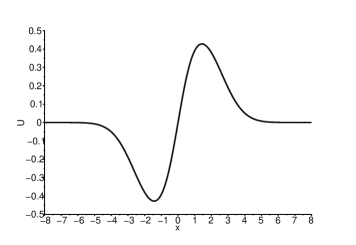
Figure 4: The profile of the antisymmetric excited state, trapped in the HO potential for $g=2$, $k=-1$, and $N=0.673$.

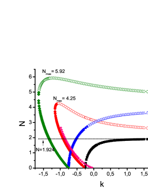
Figure 5: Numerically obtained $N(k)$ dependences for symmetric modes trapped in the HO potential, at $g=0$ (black, squares) and $g=2$ (red, circles), and for antisymmetric ones at $g=0$ (blue, triangles) and $g=2$ (green, turned squares). The TFA solutions for $g=2$ are designated by pink stars. The third and higher order modes are not included here.

The largest value of dependence $N(k)$ increases with the mode’s number, i.e., the maximum of the green branch (antisymmetric mode) exceeds the maximum of the red one (symmetric mode). Furthermore, the plots presented in Fig. 5 demonstrate additional instability of the antisymmetric modes, in comparison with their fundamental symmetric counterparts (which is not surprising, as excited states in nonlinear systems are usually more prone to instability Borovkova et al. (2011a, b)). This instability concerns the forward-going branches, that satisfy the VK criterion. The respective perturbation eigenvalues are complex, on the contrary to the pure imaginary ones that could account for the instability of the symmetric states, as mentioned above, hence they definitely cannot be detected by the VK criterion, which is, generally, less relevant for excited states, in comparison with the ground state. The predicted instability was verified by direct simulations. It was found that the instability destroys the antisymmetry of the stationary mode, and one of the two resulting peaks develops the collapse, see Fig. 6.

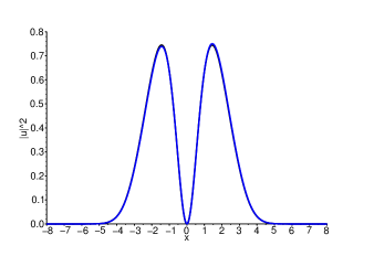
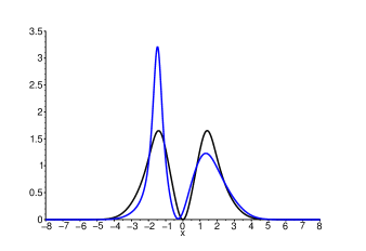
Figure 6: Stable (a) and unstable (b) evolution of an antisymmetric state trapped in the HO potential, for $g=2$, $k=-1.53$, $N=3.067$, and $g=2$, $k=-1.53$, $N=5.657$, respectively (both solutions have the same $k$ but belong, severally, to different branches: backward-going and forward-going). The initial slightly perturbed stationary state and the final one are shown by the black and blue curves, respectively.

Results concerning stability of the fundamental and antisymmetric states, obtained numerically, are collected in the diagram displayed in Fig. 7, in the plane of the norm and SDF cubic coefficient, $g$. Note that the stability area expands with the increase of $g$. Indeed, in the limit of the dominant SDF nonlinearity, there is no apparent reason for destabilization of the fundamental and excited states, which are obviously stable in the linear system. Furthermore, the strengths of the destabilizing SF and stabilizing SDF terms in Eq. (1), for modes with width $a_{\perp}\sim\Omega^{-1/4}$ and large squared amplitude $A^{2}\sim N/a_{\perp}$, balance each other at $N\sim g$, which explains the asymptotically linear shape of the stability boundaries at large $N$ in Fig. 7. On the other hand we observe that the stability intervals for both the ground state and the antisymmetric mode do not vanish in the case the SF quintic-only interaction, $g=0$.

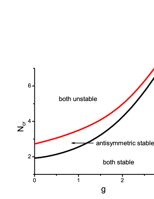
Figure 7: Stability boundaries, $N_{\mathrm{cr}}(g)$, for the fundamental (black) and first antisymmetric (red) modes trapped in the HO potential.

IV Analytical solutions for the delta-functional trapping potential

If the HO trapping potential in Eq. (4) is replaced by the delta-functional potential (7), then the respective stationary equation (9) is replaced by

$$-kU+\frac{1}{2}U^{\prime\prime}-gU^{3}+U^{5}=-\epsilon\delta(x)U$$ (18)

(recall we have fixed $\epsilon=0.5$ by means of rescaling), which implies that the jump condition (8) for symmetric solutions, with $U(-x)=U(x)$, reduces to

$$U^{\prime}(x=+0)=-\epsilon U(x=0).$$ (19)

Using exact solution (2) of Eq. (18) in the free space (at $x\neq 0$), one can easily construct the following exact solution for the mode pinned to the delta-functional potential:

$$U(x,k)=\sqrt{\frac{2\sqrt{3}k}{\sqrt{4k+3g^{2}/4}\cosh{[2\sqrt{2k}(|x|+\xi(k))]}-\left(\sqrt{3}/2\right)g}},$$ (20)

where $\xi(k)>0$ is determined by the boundary condition (19):

$$\xi(k)=\frac{1}{2\sqrt{2k}}\arcsin\left[-\frac{\sqrt{3\left[8k^{2}+({3/2})g^{2}k\right]}g\epsilon}{\left[8k+({3/2})g^{2}\right](2k-\epsilon^{2})}\right.$$

$$\left.\pm\frac{\sqrt{3\left[8k^{2}+({3/2})g^{2}k\right]g^{2}\epsilon^{2}+16k\epsilon^{2}\left[8k^{2}+({3/2})g^{2}k-4k\epsilon^{2}-({3/4})g^{2}\epsilon^{2}\right]}}{\left[8k+({3/2})g^{2}\right](2k-\epsilon^{2})}\right].$$ (21)

While at $k>0$ solution (20) is exponentially localized, in the limit of $k=0$ remains relevant, and it produces a pair of weakly localized pinned modes:

$$U(x,k = 0)=\frac{1}{\sqrt{g\left(|x|+\xi\right)^{2}+\frac{2}{3g}}},$$

$$\xi = \frac{1}{2\epsilon}\pm\sqrt{\frac{1}{4\epsilon^{2}}-\frac{2}{3g^{2}}}.$$ (22)

Obviously, this pair exists if $g$ is large enough:

$$g\geq g_{\mathrm{cr}}=2\sqrt{2/3}\epsilon\approx 0.816,$$ (23)

where the value $\epsilon\equiv 0.5$ adopted above is substituted. The weakly localized modes are meaningful ones as their norm converges, see below. Note that the weakly localized state (22) with $\xi=0$ is a valid solution to Eq. (18) in the free space, i.e., with $\epsilon=0$, but in the latter case this solution is unstable Micallef et al. (1996).

Examples of generic solutions (20), and the weakly localized ones (22), featuring a cusp at $x=0$, are displayed in Figs. 8(a) and 8(b), respectively.

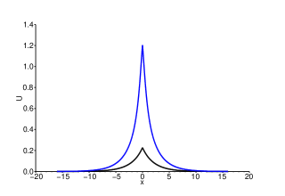
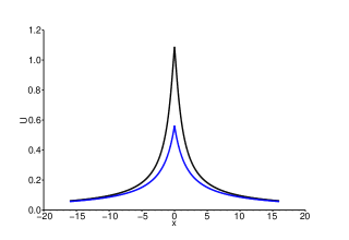
Figure 8: Exact stable solutions for the delta-functional potential (7), with $\epsilon=0.5$, (a) given by Eqs. (20) and (21) with negative (black) and positive (blue) signs for $g=1,k=0.1$, as well as (b) given by Eq. (22) for $g=1,k=0$ with both signs (black and blue profiles correspond to the solutions with “-” and “+”, respectively).                                                                                                                                                             .

At $k>0$, the analytical solution given by Eqs. (20) and (21) seems quite complex. It takes substantially simpler form for the particular case of the quintic-only nonlinearity, $g=0$:

$$U_{g=0}(x,k) = \left(3k\right)^{1/4}\sqrt{\mathrm{sech}\left(2\sqrt{2k}\left(|x|+\xi\right)\right)},$$

$$\xi = \frac{1}{2\sqrt{2k}}\mathrm{Artanh}\left({\frac{\epsilon}{\sqrt{2k}}}\right).$$ (24)

Obviously, this solution exists for sufficiently large propagation constants,

$$k>k_{\min}\equiv\epsilon^{2}/2.$$ (25)

In the opposite limit of the dominating SDF cubic term with large $g$, when the quintic term may be omitted in Eq. (18), the general solution given by Eqs. (20) and (21) also simplifies:

$$U_{g\rightarrow\infty}(x) = \sqrt{\frac{2k}{g}}\frac{1}{\sinh\left(\sqrt{2k}\left(|x|+\xi\right)\right)},$$

$$\xi = \frac{1}{\sqrt{2k}}\mathrm{Artanh}\left({\frac{\sqrt{2k}}{\epsilon}}\right).$$ (26)

Its existence region is complementary to that given by Eq. (25):

$$k\leq k_{\max}\equiv\epsilon^{2}/2.$$ (27)

Solution (26) with zero propagation constant, $k=0$, corresponds to a weakly localized mode,

$$U_{g\rightarrow\infty}(x,k=0)=\frac{1}{\sqrt{g}\left(|x|+\epsilon^{-1}\right)},$$ (28)

which is the limit case (for large $g$) of the above solution (22).

The norm of the general solution, given by Eqs. (20) and (21), is equal to

$$N(k)=\frac{2\sqrt{2k}B}{g}\left\{\frac{1}{\sqrt{1-B^{2}}}\left[\arcsin B+\arcsin\left(\frac{1-B\cosh(2\sqrt{2k}\xi)}{\cosh(2\sqrt{2k}\xi)-B}\right)\right]\right\},$$ (29)

where $B\equiv g\sqrt{3/\left(16k+3g^{2}\right)}$. In the limit of $k=0$ [provided that $g$ exceeds the critical value (23)], the norm of the weakly localized solution (22) can be found in a more explicit form,

$$N(k=0)=\sqrt{6}\left[\frac{\pi}{2}-\arctan\left(\sqrt{\frac{3}{2}}g\xi\right)\right].$$ (30)

Furthermore, in the case of the quintic-only nonlinearity, $g=0$, when the solution amounts to Eq. (24), expression (29) reduces to

$$N_{g=0}(k)=\sqrt{6}\left\{\frac{\pi}{2}-\arctan\left[\exp\left(\mathrm{Artanh}\left({\frac{\epsilon}{\sqrt{2k}}}\right)\right)\right]\right\}.$$ (31)

In the other above-mentioned limit, of large $g$, when the solution takes the form of Eq. (26), the respective simplification of expression (29) for the norm reads

$$N_{g\rightarrow\infty}(k)=\frac{2}{g}\left(\epsilon-\sqrt{2k}\right).$$ (32)

Note that Eq. (32) at $k=0$ matches Eqs. (30) and (22) in the limit of large $g$.

To check the stability of these solutions, the VK criterion can be applied first. For the case of the purely SF (quintic-only) nonlinearity, $g=0$, when this criterion is definitely relevant, Eq. (31) yields

$$\frac{dN}{dk}=\frac{\sqrt{3}\epsilon}{4\sqrt{1-(\epsilon^{2}/2k)}}k^{-3/2},$$ (33)

which is always positive in its existence range (25), hence the corresponding family of solution is entirely stable. In the general case, with $g>0$, the $N(k)$ dependence is plotted in Fig. 9(a) and 9(b) (in a smaller range).

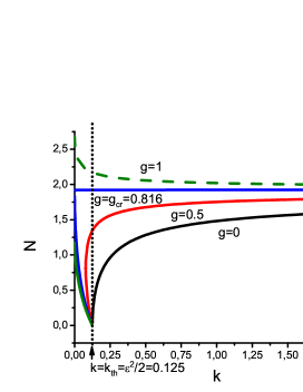
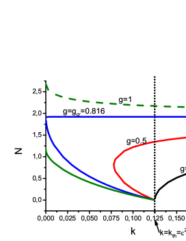
Figure 9: (a) The norm of the exact solution trapped in the delta-functional potential (7) vs. the propagation constant for different values of strength $g$ of the SDF cubic term. Unstable branches are shown by dashed lines. (b) The same as (a) in a smaller range of $k$. (c) The existence area for the solutions in the $\left(k,g\right)$ plane. (d) The stability boundary, shown as the critical norm vs. the SDF strength, $g$.

We notice in Figs. 9(a) and 9(b) that the branches produced by $``+"$ sign in Eqs. (20) and (21),which are located below the blue line corresponding to the critical value $g=g_{\mathrm{cr}}$ given by Eq. (23), entirely satisfy the VK criterion, while at $g>$ $g_{\mathrm{cr}}$ they are entirely VK-unstable, featuring $dN/dk<0$. In all forward-going branches predicted by Eqs. (20) and (21) with the $``+"$ sign, point $k=k_{\mathrm{th}}\equiv\epsilon^{2}/2=0.125$ is a singular one. On the other hand, backward-going branches corresponding to $``-"$ in Eq. (21) do not satisfy the VK criterion, hence they are either completely unstable or satisfy the anti-VK criterion, similar to the HO case. Their stability has been confirmed by the numerical verification, hence for them the anti-VK criterion indeed guarantees the stability. All the existing solutions (stable and unstable) are plotted in Fig. 9(c), including the special ones predicted by Eqs. (22) for $k\rightarrow 0$. Below $k=k_{\mathrm{th}}$, the existence area is limited by

$$k=\frac{\epsilon^{2}}{2}-\frac{3g^{2}}{16}$$ (34)

which can be derived from Eq. (21) as the boundary of physical solutions. Above $k_{\mathrm{th}}$, only the solution given by Eq. (21) with the positive sign exists, its negative counterpart being unphysical. In the limit of $g\rightarrow\infty$, the solutions with $``+"$ sign in Eq. (21) become irrelevant, as they require condition $\xi_{(+)g\rightarrow\infty}\rightarrow 0$, which can be satisfied only in the system without the delta-functional potential. The only physical solution in this regime is the one expressed by Eqs. (20) and (21) in the case of the $``-"$ sign. In other words, in this limit there is only one physical solution which can be obtained from Eq. (26), but, as said above, the solution with the negative sign can exist only for $k<k_{\mathrm{th}}$, in agreement with condition (27).

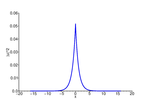
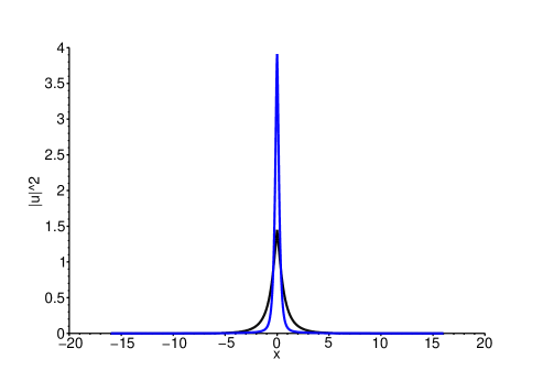
Figure 10: Examples of the perturbed evolution of stable (a) and unstable (b) modes pinned to the delta-functional potential (7), for $g=1,k=0.1,N=0.109$ and $g=1,k=0.1,N=2.193$, respectively (the same $k$, but the solution belongs to the different branches, with the $"-"$ and $"+"$ signs). The initial and final configurations are shown by the black and blue curves, respectively.

The predictions of the VK criterion for the present setting were confirmed in the case of the branches corresponding to the positive sign by numerical evaluation of eigenvalues for small perturbations, approximating, in the framework of the numerical scheme, the ideal delta-function by the Kronecker’s delta, subject to the same normalization as the delta-function. This approximation, used for the numerical evaluation of perturbation eigenvalues, as well as for direct simulations, gives very reliable results. For the stable branches, e.g., at $g=0$, all the eigenfrequencies are real, while in the case of an instability, such as the forward-going branch with the positive sign at $g\geq g_{\mathrm{cr}}$, e.g., at $g=1$, there are pure-imaginary ones. The imaginary part of the perturbations eigenvalues vanishes for backward-going branches, corresponding to the negative sign, both for $g\geq g_{\mathrm{cr}}$ and $g<g_{\mathrm{cr}}$. That conclusion confirms the anti-VK criterion for the latter branches, as they obey condition $dN/dk<0$. Furthermore, all forward-going branches below $g_{\mathrm{cr}}$ asymptotically tend to the same limit which can be easily calculated by taking the $U_{g=0}$ solution from Eq. (24) in the limit of $k\rightarrow\infty$ and its norm given by Eq. (31), $N_{g=0,k\rightarrow\infty}=\sqrt{6}\left(\pi/4\right)\approx 1.924$. This limit value is a stability boarder for all the branches with the positive and negative signs at $g<g_{\mathrm{cr}}\approx 0.816$. At $g\geq g_{\mathrm{cr}}$ the stability boundary can be found from Eq. (30) with $\xi_{(-)}$ taken as per Eq. (22). For given $g$ this is a stable solution with the largest possible value of norm (the largest-norm stable solution belongs to the backward-going branch). Obviously, there exist other solutions with still larger norms for the same $g$, but they belong to the forward-going branch, which is entirely unstable. The stability analysis presenting total norm $N$ versus the SDF strength, $g$, is summarized in Fig. 9(d).

The results were also verified by direct simulations of the perturbed evolution of the modes under consideration. Typical examples of the stable and unstable evolution are presented in Fig. 10. The unstable solution starts collapsing in the course of the evolution, similar to the system with the HO trapping potential considered above. The failure of the delta-functional pinning potential to stabilize the trapped modes at $g\rightarrow+\infty$, see Eq. (23), is a drastic difference from the case of the HO potential, where the stability of the trapped modes monotonously enhances with the increase of the strength of the cubic SDF term, $g$, see Fig. 7.

Lastly, stable solutions for solitons pinned to the attractive delta-functional potential in the model with the opposite combination of the nonlinearities, SF cubic and SDF quintic, can also be found in an analytical form. In particular, this setting gives rise to a bistability, with two different pinned states corresponding to a common value of the propagation constant Genoud, Malomed, and Weishaüpl .

V Conclusions

The aim of this work is to study, in the analytical and numerical form, the stabilization of 1D solitons by means of the external potential, under the influence of the competing SF (self-focusing) quintic and SDF (self-defocusing) cubic terms. Two standard trapping potentials were considered, the harmonic-oscillator one, and the Dirac’s delta-function. In the former case, both fundamental symmetric and the lowest antisymmetric modes were studied. In the latter, the results were obtained in the completely analytical, although somewhat cumbersome, form. The most essential result concerns the way the competing necessary stability criteria, namely, the VK (Vakhitov-Kolokolov) and anti-VK ones, divide the regions of their validity in the system with the competing nonlinear terms. In particular, in both models with the HO and delta-functional trap, the forward- and backward-going soliton branches, in terms of their dependence $N(k)$, between their norm and propagation constant, precisely obey the VK and anti-VK criteria, respectively.

It is relevant to extend the analysis for more generic forms of the trapping potential, taking into regard that the cases of the broad HO and narrow delta-functional traps produce very different results. In the 2D geometry, it may be interesting to consider the stabilization provided by trapping potentials in models combining the SF cubic nonlinearity (recall it leads to the collapse in 2D) and effectively SDF quadratic interactions. This system may be a relevant model of an optical bulk waveguide.