A novel analysis method for excited states in lattice QCD - the nucleon case

Abstract

We employ a novel method to analyze Euclidean correlation functions entering the calculation of hadron energies in lattice QCD. The method is based on the sampling of all possible solutions allowed by the spectral decomposition of the hadron correlators. We demonstrate the applicability of the method by studying the nucleon excited states in the positive and negative parity channels over a pion mass range of about 400 MeV to 150 MeV. The results are compared to the standard variational approach routinely used to study excited states within lattice QCD. The main advantage of our new approach is its ability to unambiguously determine all excited states for which the Euclidean time correlation function is sensitive on.

I Introduction

The study of excited states within the framework of Quantum Chromodynamics on the lattice (LQCD) is difficult since it is based on the evaluation of Euclidean correlation functions for which the excited states are exponentially suppressed as compared to the ground state. The standard approach to study excited states is based on the variational principle, where one considers a number of interpolating fields as a variational basis and defines a generalized eigenvalue problem (GEVP) using the correlation matrix computed within the chosen variational basis. The GEVP has been widely applied in the study of hadron spectroscopy by a number of lattice groups with recent results given in Refs. Basak et al. (2007); Gattringer et al. (2008, 2009); Mahbub et al. (2010); Bulava et al. (2010); Alexandrou et al. (2013a).

In this paper, we examine in depth the application of a new method based on statistical concepts for extracting the excited states from Euclidean correlators to study the nucleon spectrum. The so called Athens Model Independent Analysis Scheme (AMIAS)  Papanicolas and Stiliaris (2012) was originally developed to extract scattering amplitudes from experimental measurements in the $N$ to $\Delta$ transition Papanicolas and Stiliaris (2007) without utilizing a specific model thus avoiding model dependencies of the outcome. A first analysis of the nucleon two-point function in LQCD was carried out with promising results in Ref. Alexandrou et al. (2008). In this work, we extend the method to analyze correlation matrices and compare the results with those obtained in our recent study using the standard variational method Alexandrou et al. (2013a). An advantage of AMIAS is that it can be applied to the correlation function at small separation times by allowing any number of states to contribute rather than to the large time-limit behavior typically done in the variational method. In fact, the merit of the method is that it determines the actual number of states on which the correlation matrix is sensitive on. Thus AMIAS does not rely on plateau identification of effective masses, which are usually noisy and thus difficult to determine, but instead it utilizes all the information encoded in the correlation function with the advantage of exploiting the small time separations where the statistical errors are small.

The paper is organized as follows: In section II we give the general description of the method, including a discussion of an importance sampling version of the algorithm. The method is compared to standard variational approach paying particular attention to the determination of the number and correlations of the fitting parameter, which are advantages of our method. Section III gives the lattice QCD formulation pertinent to the problem at hand. Finally, in section IV, we discuss the results extracted using AMIAS and in section V we summarize our findings and give our conclusions.

II The AMIAS approach

In this section we introduce AMIAS and demonstrate its applicability in extracting the excited states from Euclidean correlation functions.

The starting point of AMIAS is a set of measurements with the associated statistical errors Papanicolas and Stiliaris (2012). Since the quantity of interest in the work is a Euclidean two-point function computed at discrete times we explain the method based on the measurement of these correlators. Let us denote by $C^{k}(t_{j}),j=1,\cdots,N_{t}$ the $k^{\rm th}$ measurement at time $t_{j}$. The next ingredient for AMIAS is a theoretical parameterization of the measurements or an ’underlining theory’. For lattice QCD correlators this is well-known from the spectral decomposition of the hadron propagator.

$$\bar{C}(t_{j})=\sum_{n=0}^{\infty}A_{n}e^{-E_{n}t_{j}}\quad.$$ (1)

The exact correlator is approximated as the average over $N$ measurements of an appropriately defined quantity to be described in Section III:

$${C}(t_{j})=\sum_{k=1}^{N}C^{k}(t_{j})$$ (2)

for a total of $N$ measurements. The parameters $A_{n}$ and $E_{n}$ are to be determined by AMIAS, where we order the exponentials by the value of $E_{n}$ $E_{0}<E_{1}<E_{2},\cdots$. For large values of the time the exponential with the smallest exponent dominates.

More details on the lattice formulation will be given in Section III.

The Central Limit Theorem states that the probability for the above average at time $t$ to have a value equal to $\bar{C}(t)$ is

$$P(\bar{C}(t_{j}))=B_{j}\exp{\left(-\frac{(\bar{C}(t_{j})-C(t_{j}))^{2}}{2(\sigma_{j}/\sqrt{N})^{2}}\right)},$$ (3)

where $\sigma_{j}$ is the standard deviation at time $t_{j}$ and $B_{j}$ is, for our purpose, an irrelevant normalization constant. The above result can be found in many textbooks and the assumptions made are that the measurements are uncorrelated and that $N$ is large. The value of $\sigma_{j}$ in Eq. (3) will, in general, be underestimated if correlations are present. For LQCD the correct value of $\sigma_{j}$ is usually obtained using either a jackknife or bootstrap procedure. An example of the distribution given in Eq. (3) for a given value of $t_{j}$ is shown in Fig. 1 showing indeed that the distribution is to a good accuracy a Gaussian. The jackknife error is found to be in agreement with that predicted by the Central Limit Theorem, which means that the measurements used for the average are uncorrelated.

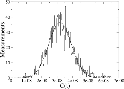
Figure 1: The correlator at a given $t_{j}$ is computed using 5000 measurements, having an average value of $C(t_{j})=3.2\times 10^{-8}$. The standard jackknife error is $1.8\times 10^{-10}$ and the weighted standard deviation is $\sigma_{j}/\sqrt{N}=1.7\times 10^{-10}$, thus demonstrating that the measurements are uncorrelated.

The probability of obtaining a set of $N_{t}$ measurements, each for a different value of $t_{j}$, is equal to the product of the probabilities for each data point:

$$\begin{split}&P(C(t_{j});\forall j=1,N_{t})=\prod_{k=1}^{N_{t}}P(C(t_{k}))\\ &=\exp{\left(-\sum_{k=1}^{N_{t}}\frac{(\bar{C}(t_{k})-C(t_{k}))^{2}}{2(\sigma_{k}/\sqrt{N})^{2}}\right)}\,,\end{split}$$ (4)

where we have set $B_{j}=1$. If we use the expansion in terms of exponentials given in Eq. (1), then the above result can be written as

$$P({C}(t_{j});\forall j = 1,N_{t})=e^{-\frac{\chi^{2}}{2}},$$ (5)

$$~{}~{}{\rm where}~{}~{}~{}\chi^{2} = \sum_{k=1}^{N_{t}}\frac{({C}(t_{k})-\sum_{n=0}^{\infty}A_{n}e^{-E_{n}t_{k}})^{2}}{(\sigma_{k}/\sqrt{N})^{2}}.$$

For practical purposes the infinite summation over the energy spectrum involving the parameters $A_{n}$ and $E_{n}$ must be truncated keeping a maximum number of $n_{\rm max}$ energy levels:

$$\chi^{2}\sim\tilde{\chi}^{2}(n_{\rm max})=\sum_{k=1}^{N_{t}}\frac{(C(t_{k})-\sum_{n=0}^{n_{\rm max}}A_{n}e^{-E_{n}t_{k}})^{2}}{(\sigma_{k}/\sqrt{N})^{2}},$$ (6)

The $\tilde{\chi}^{2}$ appearing in the above equation is the usual $\chi^{2}$ used in the least-squares fitting method. The Probability Density Function (PDF) of Eq. (5) is the basis of the $\chi^{2}$ minimization in the case where the values of the parameters are unknown: Maximizing the probability is equivalent to minimizing the exponent.

The principal idea behind AMIAS  Papanicolas and Stiliaris (2012) is that given a particular set of sampled averages, $C(t)$, any arbitrary value assigned to the parameters $A_{n}$ and $E_{n}$ constitutes a solution of Eq. 1 having the probability given by Eq. (5). Following standard statistical concepts Papanicolas and Stiliaris (2012), the probability $\Pi(a_{i})$ that the parameter $A_{i}$ assumes a specific value $a_{i}$ in the range $(b_{i},c_{i})$ is equal to

$$\Pi(a_{i})=\frac{\int_{b_{i}}^{c_{i}}\,dA_{i}\,\int_{-\infty}^{\infty}\ dE_{i}\,\int_{-\infty}^{\infty}\,\left(\prod_{\begin{subarray}{c}j=1\\ j\neq i\end{subarray}}^{n}dE_{j}dA_{j}\right)\,A_{i}e^{-\tilde{\chi}^{2}/2}}{\int_{-\infty}^{\infty}\,\left(\prod_{j=1}^{n}dA_{j}\,dE_{j}\right)\,A_{i}e^{-\tilde{\chi}^{2}/2}}.$$ (7)

The above formulation has been applied to the analysis of experimental nuclear extrapolation data Papanicolas and Stiliaris (2007) and to a lattice QCD calculation of the nucleon excited states Alexandrou et al. (2008), using a uniform sampling for values of $A_{i}\in[b_{i},c_{i})$ in Eq. (7), yielding consistent results with the standard analysis.

For reasons that will become apparent later on, instead of using a single correlation function we can apply AMIAS to a correlation matrix with the spectral decomposition

$$\bar{C}^{(i,j)}(t)=\sum_{n=0}^{\infty}A_{n}^{(i)}(A_{n}^{(j)})^{\dagger}e^{-E_{n}t}\,,\,\,\,i,j=1,\ldots,N_{\rm inter}.$$

As in the case of a single correlator we keep a maximum number of $n_{\rm max}$ energy levels in the sum.

The method can be applied to a general matrix and in the analysis where we apply AMIAS we will be interested in correlation matrices that are hermitian. This constrains the number of amplitudes $A^{(i)}$, simplifying the fitting problem. Although the matrix elements can be correlated with each other Eq. (6) is valid for each matrix element independently, hence the PDF for the entire correlation matrix can be expressed as the product of the PDF for each matrix-element, leading to a $\chi^{2}$ that is the sum of the individual $\chi^{2}$’s:

$$\begin{split}&P(C^{(i,j)}(t_{n});\forall i,j,n)=e^{-\frac{\chi^{2}}{2}},\\ &{\rm where}~{}~{}~{}\\ &\chi^{2}=\sum_{i,j}\sum_{k=1}^{N_{t}}\frac{(C^{(i,j)}(t_{k})-\sum_{n=0}^{\infty}A^{(i)}_{n}(A^{(j)}_{n})^{\dagger}e^{-E_{n}t_{k}})^{2}}{(\sigma_{t_{k}}^{(i,j)}/\sqrt{N})^{2}}.\end{split}$$ (8)

II.1 Importance sampling

While uniform sampling works well for a single correlator, for a correlation matrix determining the fit parameters $A^{(j)}$ and $E^{(j)}$ is impractical due to the large number of parameters. One can use the Metropolis algorithm Metropolis et al. (1953) to sample more efficiently the distribution $e^{-\tilde{\chi}/2}$, through a random walk. However, the Metropolis algorithm being a local random walk has the disadvantage of getting trapped at local minima. In order to avoid this problem and ensure access to the full multidimensional space, we employ parallel tempering Swendsen and Wang (1986).

In our parallel tempering scheme we run a number $r$ of additional random walks, randomly initialized at different ‘temperatures’. Thus we have a chain of random walks sampling the sequence of PDFs:
$\{\exp(-\frac{\chi^{2}}{2}),\exp(-\frac{\chi^{2}}{2T_{1}}),\exp(-\frac{\chi^{2}}{2T_{2}}),...,\exp(-\frac{\chi^{2}}{2T_{r}})\}$, where the $T_{i}$s are the parallel tempering temperatures. Sampling the distribution histogram of each parameter is done through Eq. 7 in the usual way but only the original PDF is finally used obtained by setting $T_{i}=1$. The high temperature PDFs are generally able to sample larger phase space, whereas the exact PDF with $T=1$ whilst having precise sampling in a local region of phase space, may become trapped in local minima. Information from the high temperature walks is passed down to the low temperature ones through exchanges among ensembles. Swaps are normally attempted between systems with adjacent temperatures, $k=i$ and $k=i+1$, and are accepted with probability

$$\min\{1,\exp{\left(\left(\frac{1}{T_{i}}-\frac{1}{T_{i+1}}\right)\left(\chi^{2}(i)/2-\chi^{2}(i+1)/2\right)\right)}.\}$$ (9)

Parallel tempering is an exact method, in that it satisfies the detailed balance condition.

II.2 Number of parameters

One of the significant advantages of AMIAS is that it determines unambiguously the parameters to which the data are sensitive on i.e. it determines $n_{\rm max}$ in the truncation of the infinite sum in Eq. (6). The results obtained are then invariant under changes of $n_{\rm max}$. The strategy is to increase $n_{\rm max}$ until there is no sensitivity to the additional exponentials and thus no observable change in the sampled spectrum. In Fig. 2 we show an example of such an analysis for the nucleon correlator $C(t)$, which will be defined below. As we increase $n_{\rm max}$, additional exponential terms are identified resulting in a well defined Gaussian-like distribution for each of the $E_{n}$ parameters. We can get values for the parameters, $E_{0}$, $E_{1}$ and $E_{2}$, by fitting the distribution of each mass to a Gaussian. For exponential terms beyond the first three (e.g. those having exponents $E_{3}$ and $E_{4}$) we get a uniform distribution indicating that there is no contribution to the minimization of $\tilde{\chi}^{2}$ from these terms. We can thus safely conclude that $n_{\rm max}=4$ is a safe choice since it includes, in addition to the well determined exponentials, an additional insensitive exponential term. Table 1 gives the numerical values of the energy eigenstates corresponding to the distributions of Fig. 2, where we also compare with a standard least squares minimization algorithm. The advantage of AMIAS is in the consistency of the results even when exponential terms are included on which the data are insensitive. With the usual least squares minimization one can identify three states with an error of over 50% for the $E_{2}$. No indication as to the presence of higher states can be extracted. AMIAS on the other hand yields $E_{2}$ with a 10% error. As we increase the number of exponentials from 3 to 5 the results for the parameters on which the correlator has sensitivity remain unchanged demonstrating the robustness of the method.

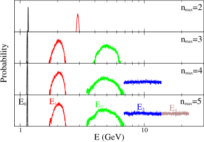
Figure 2: The Probability Density Functions (PDFs) of $E_{n}$ for different values of the truncation parameter $n_{\rm max}$ (Eq. 6). A well defined distribution is only present for the parameters that contribute to the PDF of Eq. 8. Parameters without any contribution lead to a uniform distribution.

	AMIAS			Standard Least Squares
$n_{\rm max}$	$E_{0}$	$E_{1}$	$E_{2}$	$E_{0}$	$E_{1}$	$E_{2}$
2	$1.161(13)$	$2.8990(32)$	–	$1.162(11)$	$2.92(132)$	–
3	$1.1430(32)$	$2.0453(98)$	$5.0220(53)$	$1.1439(23)$	$2.03(89)$	$5.022(2.7)$
4	$1.1430(32)$	$2.050(11)$	$4.8850(64)$	–	–	–
5	$1.1432(32)$	$2.052(11)$	$4.8394(64)$	–	–	–

Table 1: The values obtained for the ground and first two excited states of $C^{(S,S)}_{11}$ from the B55.32 ensemble. These values were obtained by a fitting a normal distribution to the results of Fig. 2. The units are in GeV.

II.3 Fit range

Figure 3: The PDFs of the energies for an eight parameter case (four amplitudes and four energies). The horizontal axis is the energy in lattice units and the vertical axis is the sampled probability of Eq. (7). The fitting range is varied by changing $t_{0}$. Exponentials with larger exponents (excited states) are suppressed but the one with smaller exponents (low-lying spectrum) remains unaffected.

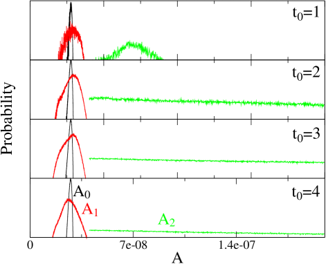
Figure 4: The PDFs of the amplitudes for an eight parameter case (four amplitudes and four masses). The horizontal axis is the amplitudes and the vertical axis is the sampled probability of Eq. (7). The fitting range is varied by changing $t_{0}$. The suppressed excited state amplitudes appear with a uniform distribution.

Another parameter that enters in the analysis of correlators is the initial time $t_{0}$ used in the fits to the exponential form. The larger the initial time the smaller is the contribution of exponentials beyond the first one. Thus, we can suppress the contribution from the higher exponents by varying the starting value $t_{0}$. In the standard analysis the time $t_{0}$ is varied until the so-called effective energy defined by

$$E_{\rm eff}(t)=\log\frac{C(t)}{C(t+1)}\stackrel{{\scriptstyle t\rightarrow\infty}}{{\longrightarrow}}E$$ (10)

becomes a constant as a function of $t$ (plateau region) yielding the lowest exponent $E_{0}$ which will be identified as the ground state energy in our lattice QCD study. Similarly, in the AMIAS analysis we need to verify that the determination of the exponents of the first exponential terms will be unaffected as we vary $t_{0}$. In Figs. 4 and 4 we show such an analysis for both $E_{n}$ and $A_{n}$ is performed. By increasing $t_{0}$ the three exponential with exponent $E_{2}$ is eliminated but the previous two exponents remain unaffected. Elimination of the third exponent is also apparent when examining the distribution of the amplitudes where the distribution of $A_{2}$ becomes uniform as $t_{0}$ is increased. Therefore, by increasing $t_{0}$ one removes unnecessary correlations from terms that we cannot clearly obtained within the available statistics and in addition, one verifies the validity of the sampled dominant exponentials.

II.4 Correlations

A central issue that is properly treated in AMIAS, is the handling of correlations, since all possible correlations are accounted for. The sampling method of Eq. (7) allows all fit parameters to randomly vary and to yield solutions with all allowed values, including the insensitive exponential terms. The visualization of the dominant correlations can be accomplished by a two-dimensional contour plot in which the values of a selected pair of parameters is varied around the region of maximum probability, keeping all other parameters fixed. In Fig. 5 we present such a correlation analysis, where the plane defined by the values of the parameters is color coded according to the $\chi^{2}$-value. The top-left and bottom-left parts are examples where the parameters are correlated, while the right part is an example of uncorrelated parameters. In particular the bottom-right part is an example where sampling is insensitive to one of the parameters, namely $E_{4}$, indicating in this case the absence of a fourth state (compared with Fig. 2).

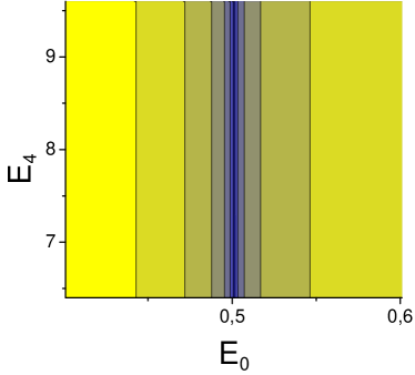
Figure 5: Contour plots showing correlations among the parameters. The contours are color coded according to the $\chi^{2}$-value. The actual data used correspond to the nucleon correlator $C_{11}^{S,S}(t)$ of the B55.32 ensemble described in Section III.

III Lattice techniques

In this section we give a more detailed description of the lattice QCD results that will be analyzed using AMIAS.

III.1 Simulation details

We use gauge configurations produced using the twisted mass fermion action with two degenerate light quarks ($N_{f}=2$). We also use twisted mass fermion gauge configurations adding to the light quarks a strange and charm quark with masses fixed to their physical values ($N_{f}=2+1+1$). More details on the $N_{f}=2+1+1$ gauge configurations produced by the European Twisted Mass Collaboration (ETMC) can be found in Ref. Baron et al. (2010) and for the $N_{f}=2$ in Ref. Boucaud et al. (2008). The twisted mass fermion ensembles used in this work are summarized in Table 2. The pion mass values span a range from about 210 MeV to 450 MeV. Apart from the twisted mass fermion ensembles we also analyze an ensemble of $N_{f}=2$ clover fermion gauge configurations produced by the QCDSF collaboration with near-physical pion mass of $m_{\pi}\simeq 160$ MeV Bali et al. (2013). The nucleon excited states have been analyzed on these gauge configurations using the conventional approach in Ref. Alexandrou et al. (2013a) and thus serve as a good set for making detailed comparison with the results obtained with AMIAS.

$N_{f}=2$ ensembles
Twisted mass fermions, $a=0.0855(6)$ fm.
$32^{3}\times 64$,	$m_{\pi}$ (GeV)	0.2696(9)	0.3082(6)
$L=2.74$ fm	No. of confs	659	232
clover fermions, $a=0.0728(5)(19)$ fm.
$48^{3}\times 64$,	$m_{\pi}$ (GeV)	0.160
$L=2.8$ fm	No. of confs	250
$N_{f}=2+1+1$ ensembles, $a=0.0863$ fm
$32^{3}\times 64$,	$m_{\pi}$ (GeV)	0.375162
(B55.32)	No. of confs	5000

Table 2: The ensembles used in our analysis.

III.2 Correlator functions

In order to study the energy spectrum within the framework of lattice QCD one evaluates the Euclidean two-point correlation function $C(t)$

$$C({\bf p},t) = \sum_{\bf x}e^{i{\bf p}.{\bf x}}<J({\bf x},t)J^{\dagger}({\bf 0},0)>$$ (11)

$$= \sum_{n=0}^{\infty}A_{n}e^{-E_{n}(p)t}\quad.$$

where $J^{\dagger}({\bf x},t)$ is a creation operator acting on the QCD vacuum (interpolating field) having the same quantum numbers as the states of interest and ${\bf p}$ is the three-momentum. The two-point correlation function can be expressed as a sum of the energy eigenstates of QCD that exponentially decay as a function of time with an exponent that depends on the energy of the state. Thus by fitting to such a form one can in principle extract the energies $E_{n}$ of the system. The problem, however, is that the higher excited states decrease exponentially as compared to the ground state and extracting them is difficult since the signal to noise decreases exponentially for all hadrons except the lowest mass pseudoscalar. Fitting such correlation functions to two-exponentials can be one approach to extract the first excited state when one has lattice data with small enough errors. On the other hand, extracting the ground state is much easier since asymptotically it is the only state that survives the large time limit of $C({\bf p},t)$.

Let us consider the zero momentum correlator $C(t)$ obtained from Eq. (1) by setting ${\bf p}={\bf 0}$. In a simulation we have $N$ measurements at each time $t$, with the $k^{\rm th}$ measurement having the form $\{C^{k}(t_{1}),C^{k}(t_{2}),...,C^{k}(t_{N_{t}})\}$, where $N_{t}$ is the number of lattice time slides on which the correlator is evaluated. Note that from now on we drop the discrete index on $t$. The $N$ measurements are over a representative ensemble of gauge configurations generated via a Monte-Carlo sampling of the probability density function of the Euclidean lattice QCD action. For each value of $t$ we can form the average $C(t)=\frac{1}{N}\sum_{k=1}^{N}C^{k}(t)$, which was the example used in the previous section to illustrate AMIAS.

The results shown in Figs. 4, 4 and 5 are carried out using the B55.32 ensemble of $N_{f}=2+1+1$ twisted mass fermions of a pion mass $m_{\pi}=373$ MeV, for which a large number of gauge configurations are generated. We will use this ensemble to perform a detailed comparison of AMIAS with the standard analysis used in lattice QCD for the study of excited states.

The standard method to study excited states in lattice QCD is the variational approach. One expands the basis to $N_{\rm inter}$ interpolating fields of the quantum numbers of states of interest and construct a correlation matrix. In this work we consider a correlation matrix of the form

$$\begin{split}&C^{\pm,(i,j)}_{ab}({\bf p},t)=\sum_{\bf x}e^{i{\bf p}.{\bf x}}\textrm{Tr}[\frac{1}{4}(1\pm\gamma_{0})\langle J_{a}^{(i)}({\bf x},t)\bar{J}_{b}^{(j)}({\bf 0},0)\rangle]\\ &=\sum_{n=0}^{\infty}e^{-E_{n}t}\textrm{Tr}[\frac{1}{4}(1\pm\gamma_{0})\langle 0|J_{a}^{(i)}|n\rangle\langle n|J_{b}^{(j)}|0\rangle]\,,&\\ &\begin{array}[]{l}i,j=1,\ldots,{N_{G}}\\ a,b=1,2,\end{array}\end{split}$$

where we denote the different types of interpolating fields with two type of indices $i,j$ and $a,b$. The superscripts $i,j$ on the correlation matrix $C^{\pm}(t)$ correspond to different levels of Gaussian smearing, while the subscripts $a,b$ to different spin combinations of the nucleon interpolating fields given by:

$$J_{1}^{(i)}=(u^{\rm T\,i}C\gamma_{5}d^{i})u^{i}\,\,\,{\rm and}\,\,\,J_{2}^{(i)}=(u^{\rm T\,i}Cd^{i})\gamma_{5}u^{i}.$$ (12)

Gaussian smearing is applied to the quark fields using the hopping matrix $H(\vec{x},\vec{y};U(t))$:

$$u^{(a,i)}(t,\vec{x}) = \sum_{\vec{y}}F^{ab}(\vec{x},\vec{y};U(t))\ u^{b}(t,\vec{y})\,,$$ (13)

$$F = (\mathbb{1}+{a_{G}}H)^{N_{G}}\,,$$

$$H(\vec{x},\vec{y};U(t)) = \sum_{i=1}^{3}[U_{i}(x)\delta_{x,y-\hat{\imath}}+U_{i}^{\dagger}(x-\hat{\imath})\delta_{x,y+\hat{\imath}}]\,.$$

We also apply APE-smearing to the gauge fields $U_{\mu}$ entering $H$. The parameters for the Gaussian smearing $a_{G}$ and $N_{G}$ are optimized using the nucleon ground state Alexandrou et al. (2013b). The local nucleon interpolator, $J_{1}^{(i)}$, is well known to have a good overlap with the ground state of the nucleon. The trace in Eq. (III.2) is taken over Dirac indices and the correlation matrices $C^{+}(t)$ and $C^{-}(t)$ yield the positive and negative parity states of the nucleon, respectively. The states $|n\rangle$ are eigenstates of the Hamiltonian with $E_{n}<E_{n+1}$ and we assume that the temporal extent of the lattice is large enough to neglect boundary contributions.

Figure 6: The PDFs for the ground and excited energies (top) and amplitudes (bottom) for smeared-smeared and local-smeared, correlators using the B55.32 ensemble. As expected the amplitudes depend on the smearing level while the energies are statistically equivalent (a reduction in the level of smearing leads to more well defined distributions for the excited states).

The low-lying energy spectrum should be unaffected by what nucleon interpolating field is used and in particular how much smearing is applied as determined by the parameters $N_{G}$ and $\alpha_{G}$. This is because Gaussian smearing only effects the coupling of the interpolating field with the nucleon eigenstates $|n\rangle$ i.e. only the $A_{n}^{i}$ are affected but not the $E_{n}^{i}$. As long as the amplitudes are non-zero the energy of interest can be extracted. In Fig. 6 we verify the independency of the energies by comparing the results from a smeared-smeared correlator $C^{(S,S)}$ where both interpolating fields in Eq. (II) are smeared to results extracted from a local-smeared correlator $C^{(L,S)}$, where only the interpolating field at the source is smeared. We show results for the ground and first excited states. As expected the distributions for $E_{0}$ and $E_{1}$ are statistically equivalent but the local-smeared correlator provides a better estimate for the excited state since it has less overlap with the ground state. In contrast, the amplitudes $A_{0}$ and $A_{1}$ depend on the level of smearing. This is an indication that reducing smearing will improve the results extracted for the excited states, since their contribution to the correlator will be larger.

III.3 Comparison of AMIAS with the variational method

The standard way to extract the ground state energy in lattice QCD is to probe the long time-limit of the correlation function and consider the effective energy $E_{\rm eff}(t)$, which becomes independent of $t$ when the ground state is the dominant contribution to the correlator. Fitting the effective energy (or mass) to a constant in the plateau region yields the ground state energy (or lowest mass). As has already been demonstrated in Ref. Alexandrou et al. (2008), the value obtained with AMIAS for the ground state is in agreement with the one extracted from the effective mass plateaus. In this section, we focus our attention to the extraction of the excited states.

In order to study excited states in lattice QCD, one usually applies the variational method and defines a generalized eigenvalue problem (GEVP) given by

$$\begin{split}&C(t)v_{n}(t,t_{i})=\lambda_{n}(t,t_{i})C(t_{i})v_{n}(t,t_{i}),\hskip 14.22636pt\\ &n=1,\ldots,N,\,t>t_{i}\,,\end{split}$$ (14)

where $E_{n}=\lim_{t\rightarrow\infty}-\partial_{t}\log\lambda_{n}(t,t_{i})$. The corrections to $E_{n}$ decrease exponentially like $e^{-\Delta E_{n}t}$ where $\Delta E_{n}=\min_{m\neq n}|E_{m}-E_{n}|$ Lüscher and Wolff (1990) for fixed $t_{i}$. In a recent application of the variational method for the analysis of the nucleon states Alexandrou et al. (2013a) we found that a variational basis constructed from different smearing levels of the standard interpolating field $J_{1}$ containing both a small and a large number of Gaussian smearings $N_{G}$ is an appropriate basis for extracting the first positive parity excited state, known as the Roper.

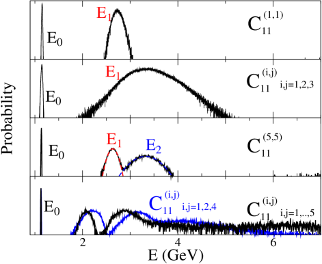
Figure 7: The spectrum from AMIAS when using the diagonal $C_{11}^{(1,1)}$ and $C_{11}^{(5,5)}$ correlators as well as the $3\times 3$ correlation matrices $C_{1,1}^{(i,j)},\,i,j=1,2,3$ and $C_{1,1}^{(i,j)},\,i,j=1,2,4$. Results are also shown for the $5\times 5$ matrix $C_{1,1}^{(i,j)},\,i,j=1,\ldots,5$. The inclusion of a variational basis that includes small and large smearings leads to an improved excited-state spectrum.

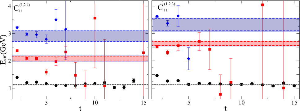
Figure 8: The points show the effective masses determining from the GEVP analysis while the bands show the values obtained by AMIAS for the same correlation matrix. The left panel shows results extracted the $3\times 3$ correlation matrix $C_{11}^{(1,2,4)}$, while the left panel from the $3\times 3$ correlation matrix, $C_{11}^{(1,2,3)}$.

In order to compare AMIAS with the results extracted using GEVP, we consider the same variational basis used in that study, namely we set the values of the smearing parameters to $\alpha_{G}=4.0$ and $N_{G}=$10, 30, 50, 180 and 300. These different smearing levels are labeled by the superscript $i=1,\ldots,5$ on $J_{a}^{(i)}$ and produce a source with a root mean square radius $2.26a,~{}3.77a,~{}4.77a,~{}8.37a$ and $10.19a$ in units of the lattice spacing $a$, respectively. The resulting matrices are symmetrized. For this analysis, we use 200 twisted mass configurations produced at $\beta$=3.9, a$\mu$ = 0.004 or m${}_{\pi}\sim 308$ MeV on a 32³ $\times$ 64 lattice. In Fig. 7 we show the results extracted from AMIAS for the various correlation matrices. The value for the first excited state obtained from fitting the diagonal elements is statistically equivalent for all values of the smearings. This is illustrated in Fig. 7, where we show the results extracted from $C_{1,1}^{(1,1)}$ and $C_{1,1}^{(5,5)}$, which correspond to the smallest and largest smearings, respectively. When a correlation matrix is used there is a lowering in the value of the first excited state and in addition a second excited state appears close-by. This indicates that this state cannot be detected in the diagonal correlators, presumably having a very small overlap within the standard nucleon interpolating field. A $3\times 3$ correlation matrix using the first three smearing levels $C_{1,1}^{(i,j)},\,i,j=1,2,3$ is compared with a $3\times 3$ matrix, $C_{1,1}^{(i,j)},\,i,j=1,2,4$. Using a variational basis that includes small and large smearings i.e $N_{G}=10$ and $N_{G}=300$ results in a lowering of the energy of the first excited state. Furthermore, using the full $5\times 5$ correlation matrix, $C_{1,1}^{(i,j)},\,i,j=1,\ldots,5$, results in a reduction of the error but leaves the mean values unaffected.

We compare the results extracted with AMIAS to the effective energies extracted from GEVP in Fig. 8. The AMIAS values are shown by the bands, while the effective mass by the symbols. As can be seen, the effective energies as a function of the time separation become very noisy for the first and second excited states making the identification of the plateau region ambiguous. AMIAS nicely extracts these energies, which are in agreement with the levels that the variational approach seems to indicate. This illustrates the advantage of AMIAS in the determination of the excited states.

IV The low-lying nucleon spectrum

Having presented a detailed comparison with the results obtained by using GEVP, in this section we present the results for the nucleon excited states in the positive- and negative-parity channels obtained by applying AMIAS. For this analysis we use the $4\times 4$ correlation matrix $C_{ab}^{(i,j)},~{}~{}a,b=1,2~{}~{}i,j=3,4$. These correlation matrices were also utilized within the GEVP analysis of Ref. Alexandrou et al. (2013a) and thus readily provide a comparison with the results obtained within the AMIAS analysis.

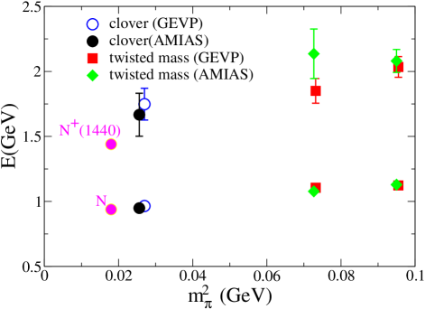
Figure 9: The nucleon ground state and first excited state in the positive parity channel. The values obtained using AMIAS (filled back circles and filled green diamond) are compared to the results extracted from GEVP Alexandrou et al. (2013a).

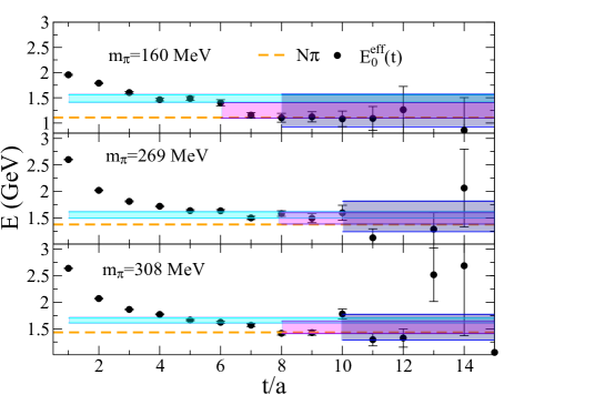
Figure 10: The effective mass for the negative parity ground state for all of our ensembles. Shaded error bands obtained by AMIAS for various values of $t_{0}$ are shown. The dotted line indicates the $N\pi$ ground state energy which is obtained from the sum of the nucleon and pion masses for the particular ensemble.

Figure 11: The same as in Fig. 9 but for the negative parity channel.

In Figs. 9 and 11 we show the results for both positive and negative parity states, for the twisted mass ensembles and for the clover ensemble analyzed in this work. The results are compared with those obtained using the GEVP. For the case of the clover action and the heaviest of the twisted mass ensembles ($m_{\pi}=0.3082(6)$GeV) we have refined our analysis by expanding the basis of the GEVP as compared to the analysis carried out in Ref. Alexandrou et al. (2013a). For these two ensembles the results obtained with AMIAS are consistent with the GEVP. For the twisted mass ensemble with the smaller pion ($m_{\pi}=0.2696(9)$GeV) the first excited state obtained with AMIAS has a larger error than the one extracted from the plateau. This is because in the GEVP one needs to fit for small $t_{0}$ in order to have enough fitting points. Contrary in AMIAS we utilize the whole time dependence and thus we are more confident for the AMIAS determination.

For the negative parity channel there is an interesting feature connected to the $N\pi$ scattering state. Unlike the behavior observed in the positive channel where AMIAS yields results that did not show any dependence on $t_{0}$ here this is no longer the case. The lowest level extracted when using $t_{0}/a=1$ is higher that the energy of the S-wave $N\pi$ scattering state assuming that no interactions take place. AMIAS yields results in agreement with the GEVP only after increasing the value of $t_{0}$, albeit with larger errors. This was further investigated in Fig. 10, where we show the effective mass for the negative parity ground state for the three lowest pion masses used. The values extracted using AMIAS for various starting values of the fit range, $t_{0}$ are shown by the shaded error bands as $t_{0}$. The values of $t_{0}$ used are indicated by the timeslice where the bands start. The dashed line shows the energy of the scattering state being the sum of the pion and nucleon mass. As can be see, with increasing $t_{0}$ the error band width increases becoming consistent with the mass of the $N\pi$ scattering state but at the same remains consistent with the band obtained with $t_{0}/a=1$. This is consistent with our analysis in section II.3 where we have shown that increasing $t_{0}$ suppresses excited states but does not affect the mean value of the ground state. One possible reason that one needs to increase $t_{0}$ to obtain agreement with the $N\pi$ energy maybe the small overlap this two-particle state may have with a single particle interpolating field, requiring the suppression of the excited states to get a signal and may explain why other groups have not been able to detect it. In Fig. 11 we give the values extracted for the ground and the first excited state in the negative channel. The values shown for the $N\pi$ correspond to the magenta bands in Fig. 10 obtained using $t_{0}/a=6$ for clover fermions and $t_{0}/a=8$ for twisted mass fermions. In contrast, the excited state was obtained using $t_{0}/a=1$ in analogy with the positive parity channel.

V Summary and Conclusions

A novel method for the analysis of excited states within lattice QCD is applied to study the spectrum of the nucleon. The method uses importance sampling to probe the correct minimum of the multidimensional space defined by the states of the correlation matrix. AMIAS determines the number of excited states, which can be extracted from the information that the lattice data encode. It takes advantage of the whole time dependence of the correlators not requiring identification of the large time asymptot that limits the accuracy of the determination of excited states. The method is applied to successfully extract the first excited states in the positive and parity nucleon channels, identifying the Roper in the positive parity channel. In the negative parity it can extract the energy of the first excited state using the entire time dependence of the two-point function the energy of the $N\pi$ scattering state is only extracted after eliminating the initial few time slices suppressing the excited states. This is a feature that we plan to explore further in future studies.

References

- Basak et al. (2007) S. Basak, R. Edwards, G. Fleming, K. Juge, A. Lichtl, et al., Phys.Rev. D76, 074504 (2007), eprint 0709.0008.
- Gattringer et al. (2008) C. Gattringer, L. Y. Glozman, C. Lang, D. Mohler, and S. Prelovsek, Phys.Rev. D78, 034501 (2008), eprint 0802.2020.
- Gattringer et al. (2009) C. Gattringer, C. Hagen, C. Lang, M. Limmer, D. Mohler, et al., Phys.Rev. D79, 054501 (2009), eprint 0812.1681.
- Mahbub et al. (2010) M. Mahbub, A. O. Cais, W. Kamleh, D. B. Leinweber, and A. G. Williams, Phys.Rev. D82, 094504 (2010), eprint 1004.5455.
- Bulava et al. (2010) J. Bulava, R. Edwards, E. Engelson, B. Joo, H.-W. Lin, et al., Phys.Rev. D82, 014507 (2010), eprint 1004.5072.
- Alexandrou et al. (2013a) C. Alexandrou, T. Korzec, G. Koutsou, and T. Leontiou (2013a), eprint 1302.4410.
- Papanicolas and Stiliaris (2012) C. N. Papanicolas and E. Stiliaris (2012), eprint arXiv:1205.6505.
- Papanicolas and Stiliaris (2007) C. N. Papanicolas and E. Stiliaris, AIP Conf. Proc. 904, 257 (2007).
- Alexandrou et al. (2008) C. Alexandrou, C. N. Papanicolas, and E. Stiliaris, PoS LATTICE2008, 099 (2008), eprint 0810.3982.
- Metropolis et al. (1953) N. Metropolis, A. W. Rosenbluth, M. N. Rosenbluth, A. H. Teller, and E. Teller, J. Chem. Phys. 21, 1087 (1953).
- Swendsen and Wang (1986) R. H. Swendsen and J.-S. Wang, Phys. Rev. Lett. 57, 2607 (1986), URL http://link.aps.org/doi/10.1103/PhysRevLett.57.2607.
- Baron et al. (2010) R. Baron, P. Boucaud, J. Carbonell, A. Deuzeman, V. Drach, et al., JHEP 1006, 111 (2010), eprint 1004.5284.
- Boucaud et al. (2008) P. Boucaud et al. (ETM), Comput. Phys. Commun. 179, 695 (2008), eprint 0803.0224.
- Bali et al. (2013) G. Bali, P. Bruns, S. Collins, M. Deka, B. Glasle, et al., Nucl.Phys. B866, 1 (2013), eprint 1206.7034.
- Alexandrou et al. (2013b) C. Alexandrou, M. Constantinou, V. Drach, K. Jansen, C. Kallidonis, et al. (2013b), eprint 1312.2874.
- Lüscher and Wolff (1990) M. Lüscher and U. Wolff, Nucl.Phys. B339, 222 (1990).