Experimental observation of induced stochastic transitions in multi-well potential of RF SQUID loop

Abstract

An amplification of a weak low-frequency harmonic signal is experimentally observed in a single-junction-superconducting quantum interferometer (RF SQUID loop) due to stochastic transitions between two or more metastable states of the loop under the applied noise flux of varying intensity (the effect of stochastic resonance, SR). In addition to the usual scenario of the SR in a bistable system with Gaussian noise, the transitions between multiple metastable states of the multi-well SQUID loop potential under the influence of a binary noise is observed. This can be interpreted as a kind of noise ”spectroscopy” of the metastable states of the SQUID loop with different values of the trapped magnetic flux.

I Introduction

The Superconducting Quantum Interference Devices (SQUIDs) are the base element of the most currently sensitive magnetometers widely used in both physical experiments and applications (medicine, geophysics, industry). The sensitivity of the SQUIDs and their quantum analogues, SQUBIDs (Superconducting QUBIt Detectors), has practically reached the quantum limitation 1 ; 2 ; 3 . However, with increase of the temperature $T$ and the quantizing loop inductance $L$, the uncertainty of the noise flux rises thus resulting in a degradation of the energy resolution (sensitivity). This issue is the most severe for high-$T_{c}$ SQUIDs cooled down to the liquid nitrogen temperature level where the quantizing loop inductance and, correspondingly, the sensitivity to the magnetic field have to be considerably reduced. However, as shown in papers 4 ; 5 ; 6 ; 7 ; 8 ; 9 , due to the same thermodynamic fluctuations and the external noise, the sensitivity of the magnetometers can be essentially enhanced by using the stochastic resonance (SR) effect.

The SR phenomenon discovered in the early 1980s 10 ; 11 manifests itself in a non-monotonic rise of the response of a non-linear, often bi-stable, system to a weak periodic signal whose characteristics (amplitude, signal-to-noise ratio) become better at the system output. Actually, to enable the SR in a specific system, it is enough that the time duration of the system being in one of its metastable states (MS) (the residence time) would be a function of the noise intensity. The SR effect has been found in numerous natural and artificial systems, both classic and quantum; the analytical approaches, the criteria and quantifiers to estimate the noise-induced ordering were elaborated 12 ; 13 . For the aperiodic systems with strong dissipation (which are mostly explored theoretically and experimentally), the ”stochastic filtration” (SF) is rather more appropriate term than the widely accepted ”stochastic resonance” 14 . Practically all the high-$T_{c}$ SQUIDs belong here.

Although a noticeable number of the theoretical and modeling studies of the SR in the superconducting loop are published, there is still a lack of the experimental investigations of the stochastic dynamics in SQUIDs 15 (e.g., 4 ; 5 ; 6 ). Therefore some questions still remain in this field, including possible practical applications. For example, is it possible to enhance substantially the sensitivity of the high-$T_{c}$ SQUIDs with SR by an optimal choice of their parameters in the area of strong fluctuations $L\geq L_{F}=\Phi_{0}^{2}/(4\pi^{2}k_{B}T)$? Here $L_{F}$ is the fluctuation inductance, $L_{F}\sim 10^{-10}$ H at $T=77$ K, $\Phi_{0}=2.07\cdot 10^{-15}$ Wb is the superconducting magnetic flux quantum, $k_{B}$ is the Boltzmann constant. Additionally, it should be noted that even if the system has many states, usually the transitions between only two adjacent MSs are considered in the context of the SR and SF. The noise type and statistics may introduce their specifics in the stochastic dynamics of the interferometers.

In this work we experimentally observed an amplification of a weak harmonic low-frequency signal in an RF SQUID loop due to stochastic transitions between two and more metastable states of the loop induced by the Gaussian or binary noise of varying intensity (the stochastic filtration effect).

II RF SQUID dynamics and experimental

In the absence of fluctuations, the number of the local minima of the quantizing loop potential energy $u(x,x_{e})=(x-x_{e})^{2}/2-\frac{\beta_{L}}{4\pi^{2}}\cos(2\pi x)$ (the number of the loop MSs) is defined by the dimensionless parameter of non-linearity $\beta_{L}=2\pi LI_{c}/\Phi_{0}$: $n\approx\,2\beta_{L}/\pi$. Here $x_{i}=\Phi_{i}/\Phi_{0}$ and $x_{i}=\Phi_{i}/\Phi_{0}$ are the dimensionless internal and external fluxes, correspondingly, the energy is normalized to $\Phi_{0}^{2}/2L$, while $I_{c}$ is the contact critical current.

In our experiments, we tested the interferometers with large $\beta_{L}\approx 7-10$ and the low-impedance ($R\sim 1$ $\Omega$) Josephson junctions of ScS (superconductor-constriction-superconductor) type having low intrinsic capacity ($C\approx 3\cdot 10^{-15}$ F). Such a set of the parameters determine the overdamped regime which is also typical for most of the high-$T_{c}$ SQUIDs.

Taking into account the smallness of $C$ and $R$, we may neglect the second derivative in the flux motion equation 16 and reduce it to the form convenient for computations 7 ; 8 ; 9 :

$\displaystyle\frac{dx}{dt}=\frac{1}{\tau_{L}}\left[x_{e}(t)-x+\frac{\beta_{L}}{2\pi}\sin(2\pi x)\right]$,

where $\tau_{L}=L/R$ is the loop flux decay time. The equation describes an aperiodic system. The external flux $x_{e}$ is the sum of the fixed bias flux ($x_{dc}=0.5$) to symmetrize the potential, the weak low-frequency information signal $x_{s}=a\sin 2\pi f_{s}t$ ($a<<1$) and uncorrelated (white) Gaussian noise $x_{N}=\xi(t)$, $\left\langle\xi(t)\cdot\xi(t^{\prime})\right\rangle=2D\delta(t-t^{\prime})$, where $D$ is the noise intensity. However, both in the calculations and the experiments, the noise is frequency-band limited by a cut-off frequency. To consider it practically uncorrelated in the context of the discussed SR model, the cut-off frequency $f_{c}$ should sufficiently exceed the signal frequency: $f_{c}>>f_{s}$. In our experiments, we chose $f_{s}=37$ Hz and $f_{c}=50$ kHz. The used instrument generated the Gaussian or the binary (telegraph) noise originated from a real physical source (diode).

The interferometer under test (denoted by 1 in Fig. 1) was designed as a niobium 3D self-shielded toroidal construction with the adjusted point contact. It coupled to an instrumental RF SQUID magnetometer (denoted by 2 in Fig. 1) via the superconducting magnetic flux transformer with the interferometer loop-to-loop flux coupling coefficient $k=0.05$. The interferometer design is described in detail in the paper2 . The spectral density of the magnetic flux noise (the sensitivity) of the magnetometer was $S_{\Phi}^{1/2}\approx 2\cdot 10^{-4}\;\Phi_{0}/Hz^{1/2}$ within the operation frequency band of 2 to 200 Hz. The coupling coefficients, the fluxes and the coil RF currents were determined from the measurements of the amplitude-frequency and the amplitude-flux characteristics of the interferometer under test while changing the in-loop flux within $\pm 5\Phi_{0}$. The experimental setup is similar ideologically to that reported in 5 and will be described elsewhere. The measurements were taken at temperature 4.2 K inside a superconducting shield. The cryostat, in its turn, was placed into the three-layer mu-metal shield. The output signal was fed to the spectrum analyzer Bruel&Kjer 2033. The number of the instrumentally-averaged spectra was 16. The readings were taken doubly, with and without the information signal. The difference between the two spectra obtained was considered as the result.

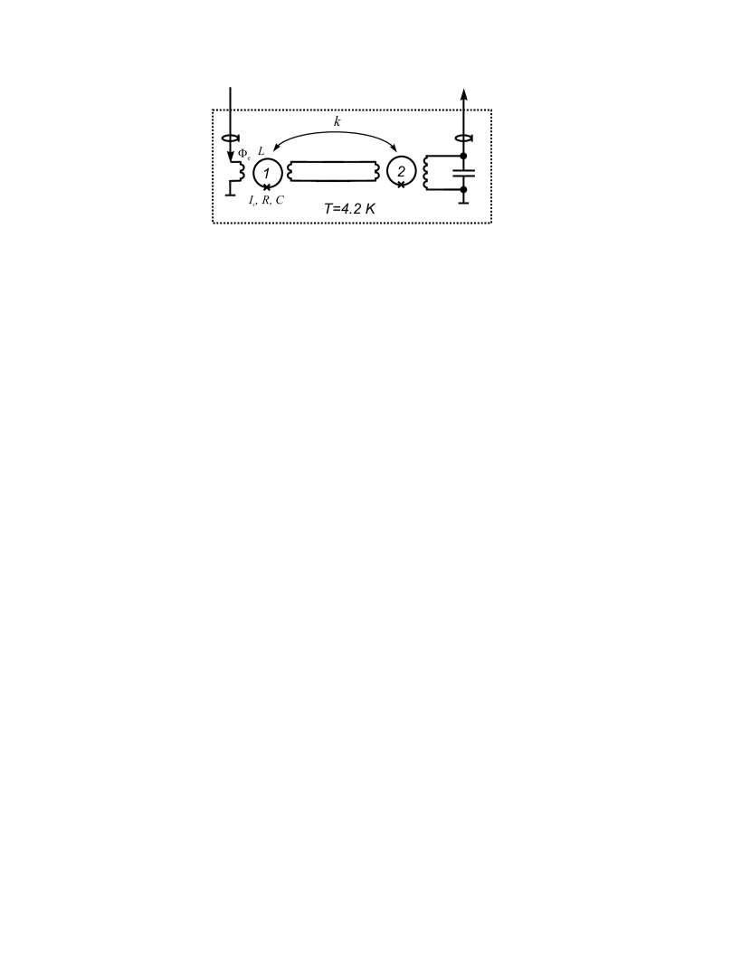
Figure 1: The simplified diagram of the measurements. External magnetic flux $\Phi_{e}$ is applied by a coil to the loop of the interferometer under test (denoted by number 1). The in-loop flux is measured with the RF SQUID magnetometer (denoted by number 2) via the superconducting magnetic flux transformer. The coupling coefficient between the loops is denoted by $k$ . The dotted line indicates the superconducting led shield.

III Results and discussion

The numerical calculations 4 ; 5 ; 7 ; 8 ; 9 show that the spectrum density of the internal flux in the SQUID loop at the useful signal frequency rapidly rises, peaks and then slowly decreases with the increase of the Gaussian noise intensity $D$, in accordance with the theory 12 ; 13 .

Fig. 2(a) exhibits the amplitude spectral density of the flux inside the interferometer loop at the information signal frequency $S_{\Phi}^{1/2}(f_{s})$ calculated numerically as a function of the mean-square amplitude of the Gaussian noise $D^{1/2}$ (solid line) along with the experimental points (solid squares). The amplitude of the harmonic signal inside the interferometer under test was $a=0.015$ in $\Phi_{0}$ units. The interferometer behavior is typical for the scenario of the SR (more accurate, SF) in a bi-stable system. The inset in Fig 2(a) displays the spectrum of the in-loop magnetic flux corresponding to the maximum signal gain. The average frequency of the noise-induced transitions between the MSs (Kramers rate 17 ) $r_{K}\approx 2f_{s}$ in this point, while the in-loop flux spectrum takes $1/f$ form. For the chosen, rather large, $\beta_{L}$ , the maximum gain of about 10 dB was obtained in this experiment.

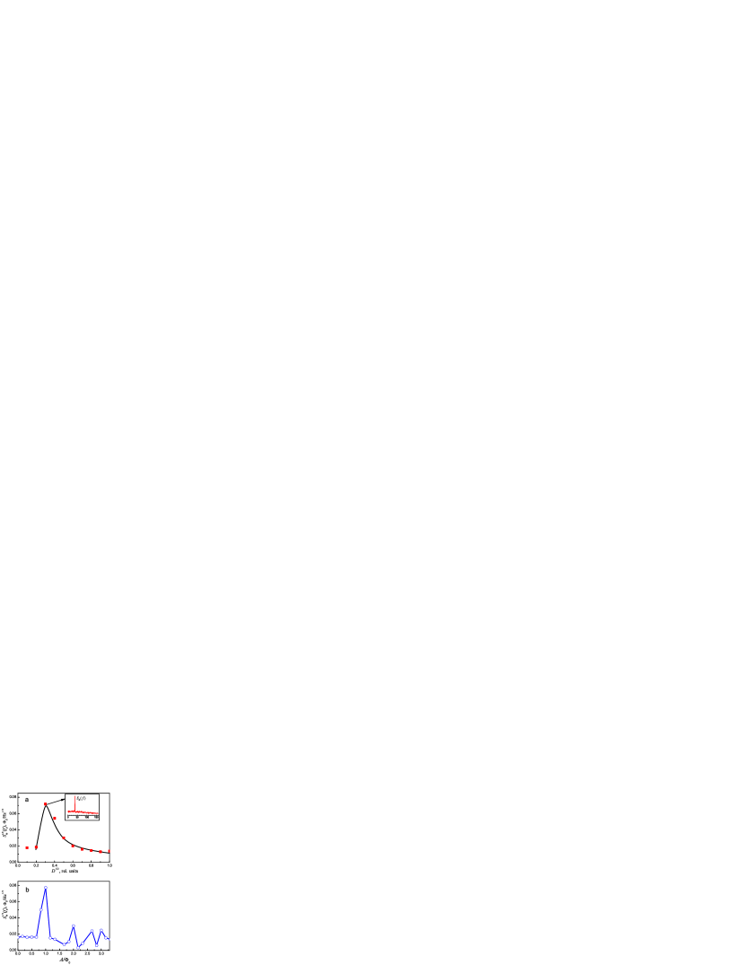
Figure 2: (Color online) The amplitude spectral density $S_{\Phi}^{1/2}$ of the magnetic flux inside the RF SQUID loop at frequency $f_{s}$ of the weak harmonic signal as a function of the mean-square amplitude $D^{1/2}$ of the Gaussian noise (solid line is the numerical calculation, solid squares are the experimental points) (a) and of the reduced amplitude $A/\Phi_{0}$ of the binary noise (hollow circles are the experimental points) (b). The inset in (a) shows the experimental spectrum of the output signal (measured in-loop flux) at the maximum signal gain.

The system demonstrates different behavior with the binary (telegraph) noise instead, whose amplitude is fixed while the phase is random. The time of the system residence in one of its MSs in the case of the Gaussian noise changes gradually with the noise intensity. Under the binary noise, the system remains in a certain MS during the noise intensity rise until the noise amplitude becomes sufficient to cause the induced transition to another MS. The ”stochastic synchronization” in this situation occurs between the useful signal phase and the random phase of the binary noise.

As it was mentioned above, the SR phenomenon is considered assuming the two MSs separated by the potential barrier with a small height to achieve larger gain. For the low-temperature SQUID, this means that $\beta_{L}$ should range from 1 to 1.5. However, the high-$T_{c}$ SQUIDs cooled down to the liquid nitrogen temperature level, in which the use of SR could be advantageous, keep quasi-nonhysteretic behavior up to $\beta_{L}\approx 3.5$ 18 ; 19 ; 20 ; 21 due to the large variance of the magnetic flux fluctuations. In this area of strong fluctuations, the number of MSs can be measured by means of the SR.

We tested the interferometer with a few MSs for the SR effect varying the amplitude of the external binary noise. Fig. 2(b) demonstrates the amplitude spectral density $S_{\Phi}^{1/2}(f_{s})$ of the in-loop magnetic flux at the useful signal frequency $f_{s}$ as a function of the amplitude $A$ of the in-loop binary noise expressed in $\Phi_{0}$ units. The signal parameters are the same as above: the frequency $f_{s}=37$ Hz, the amplitude of the in-loop flux variation $a=0.015\;\;(\Phi_{0})$. The amplitude of the in-loop magnetic noise flux ranged from 0 to $\sim 3.5\;\Phi_{0}$. It is seen from the plot in Fig. 2(b) that the additional signal gain maxima corresponding to the stochastic transitions between several MSs of the loop with the different captured flux are observed while increasing the noise amplitude. The well-determined amplitude of the telegraph noise allowed us to perform a kind of ”spectroscopy” of the MSs in the superconducting interferometer loop in the limit of strong fluctuations. The $\beta_{L}$ for this interferometer was estimated by the amplitude-frequency characteristics without an external noise as about 10.

IV Summary

The SR (or SF, for an overdamped aperiodic system) effect enables certain gain of a weak periodic signal due to ”stochastic synchronization” of the noise-induced transitions between two or more metastable states with this useful signal. This scenario is observed in the experiment with the superconducting quantum interferometer. To obtain a large enough gain (like, e.g. in 5 ) predicted theoretically (see Refs. in 4 ; 5 ; 9 ) and numerical calculations 8 ; 9 , it is necessary to optimize the SQUID parameters, particularly, use the interferometer with low $\beta_{L}\geq 1$ . For the high-$T_{c}$ RF SQUIDs in the area of strong fluctuations, the effective double-well potential and the best stochastic gain of a weak information signal should be observed at $\beta_{L}\approx 4$ .

The stochastic gain of a weak periodic signal is observed due to the noise-induced transitions not only between the two adjacent metastable current states of the superconducting interferometer loop but also between several more distant ones. The picture is more distinct in the case of the binary noise that gives grounds to consider the procedure as a specific ”noise spectroscopy” of the system metastable states.

References

- (1) M.B. Ketchen, J.M. Jaycox, Appl. Phys. Lett. 40, 736 (1982).
- (2) V.I. Shnyrkov, A.A. Soroka, and O.G. Turutanov, Phys. Rev. B 85, 224512 (2012).
- (3) V.I. Shnyrkov, A.A. Soroka, A.M Korolev, O.G. Turutanov, Low Temp. Phys. 38, 301 (2012).
- (4) R. Rouse, S. Han, J.E. Lukens, Appl. Phys. Lett. 66, 108 (1995).
- (5) A.D. Hibbs, A.L. Singsaas, E.W. Jacobs, A.R. Bulsara, J.J. Bekkedahl et al., J. Appl. Phys. 77, 2582 (1995).
- (6) A.D. Hibbs, B.R. Whitecotton, Appl. Supercond. 6, 495 (1998) .
- (7) O.G. Turutanov, A.N. Omelyanchouk, V.I. Shnyrkov, Yu.P. Bliokh, Physica C 372-376, 237 (2002).
- (8) A.M. Glukhov, O.G. Turutanov, V.I. Shnyrkov, A.N. Omelyanchouk, Low Temp. Phys. 32, 1123 (2006).
- (9) O.G. Turutanov, V.A. Golovanevskiy, V.Yu. Lyakhno, V.I. Shnyrkov, Physica A 396, 1 (2014).
- (10) R. Benzi, A. Sutera, A. Vulpiani, J. Phys. A 14, L453 (1981).
- (11) C. Nicolis, G. Nicolis, Tellus 33, 225 (1981).
- (12) L. Gammaitoni, P. Hänggi, P. Jung, F. Marchesoni, Rev. Mod. Phys. 70, 223 (1998).
- (13) V.S. Anishchenko, A.B.Neiman, F. Moss, L. Shimansky-Geier, Phys. -Usp. 42, 7 (1999).
- (14) Yu. L. Klimontovich, Phys. -Usp. 42, 37 (1999).
- (15) A.R. Bulsara, Nature 437, 962 (2005).
- (16) A. Barone, G. Paterno, Physics and Applications of the Josephson Effect, Wiley, New York, 1982.
- (17) H.A. Kramers, Physica 7, 284 (1940).
- (18) X.H. Zeng, Y. Zhang, B. Chesca et al., J. Appl. Phys .88, 6781 (2000).
- (19) B. Chesca, J. Low Temp. Phys. 110, 963 (1998).
- (20) Ya. S. Greenberg, J. Low Temp. Phys. 114, 297 (1999.).
- (21) V.I. Shnyrkov, High-Temperature RF SQUIDs. In: Handbook of High-Temperature Superconductor Electronics, ed. N. Khare, New York, Marcel-Dekker, 193 (2003).