A Latent Source Model for
Online Collaborative Filtering

Abstract

Despite the prevalence of collaborative filtering in recommendation systems, there has been little theoretical development on why and how well it works, especially in the “online” setting, where items are recommended to users over time. We address this theoretical gap by introducing a model for online recommendation systems, cast item recommendation under the model as a learning problem, and analyze the performance of a cosine-similarity collaborative filtering method. In our model, each of $n$ users either likes or dislikes each of $m$ items. We assume there to be $k$ types of users, and all the users of a given type share a common string of probabilities determining the chance of liking each item. At each time step, we recommend an item to each user, where a key distinction from related bandit literature is that once a user consumes an item (e.g., watches a movie), then that item cannot be recommended to the same user again. The goal is to maximize the number of likable items recommended to users over time. Our main result establishes that after nearly $\log(km)$ initial learning time steps, a simple collaborative filtering algorithm achieves essentially optimal performance without knowing $k$. The algorithm has an exploitation step that uses cosine similarity and two types of exploration steps, one to explore the space of items (standard in the literature) and the other to explore similarity between users (novel to this work).

1 Introduction

Recommendation systems have become ubiquitous in our lives, helping us filter the vast expanse of information we encounter into small selections tailored to our personal tastes. Prominent examples include Amazon recommending items to buy, Netflix recommending movies, and LinkedIn recommending jobs. In practice, recommendations are often made via collaborative filtering, which boils down to recommending an item to a user by considering items that other similar or “nearby” users liked. Collaborative filtering has been used extensively for decades now including in the GroupLens news recommendation system [20], Amazon’s item recommendation system [17], the Netflix Prize winning algorithm by BellKor’s Pragmatic Chaos [16, 24, 19], and a recent song recommendation system [1] that won the Million Song Dataset Challenge [6].

Most such systems operate in the “online” setting, where items are constantly recommended to users over time. In many scenarios, it does not make sense to recommend an item that is already consumed. For example, once Alice watches a movie, there’s little point to recommending the same movie to her again, at least not immediately, and one could argue that recommending unwatched movies and already watched movies could be handled as separate cases. Finally, what matters is whether a likable item is recommended to a user rather than an unlikable one. In short, a good online recommendation system should recommend different likable items continually over time.

Despite the success of collaborative filtering, there has been little theoretical development to justify its effectiveness in the online setting. We address this theoretical gap with our two main contributions in this paper. First, we frame online recommendation as a learning problem that fuses the lines of work on sleeping bandits and clustered bandits. We impose the constraint that once an item is consumed by a user, the system can’t recommend the item to the same user again. Our second main contribution is to analyze a cosine-similarity collaborative filtering algorithm. The key insight is our inclusion of two types of exploration in the algorithm: (1) the standard random exploration for probing the space of items, and (2) a novel “joint” exploration for finding different user types. Under our learning problem setup, after nearly $\log(km)$ initial time steps, the proposed algorithm achieves near-optimal performance relative to an oracle algorithm that recommends all likable items first. The nearly logarithmic dependence is a result of using the two different exploration types. We note that the algorithm does not know $k$.

Outline. We present our model and learning problem for online recommendation systems in Section 2, provide a collaborative filtering algorithm and its performance guarantee in Section 3, and give the proof idea for the performance guarantee in Section 4. An overview of experimental results is given in Section 5. We discuss our work in the context of prior work in Section 6.

2 A Model and Learning Problem for Online Recommendations

We consider a system with $n$ users and $m$ items. At each time step, each user is recommended an item that she or he hasn’t consumed yet, upon which, for simplicity, we assume that the user immediately consumes the item and rates it $+1$ (like) or $-1$ (dislike). The reward earned by the recommendation system up to any time step is the total number of liked items that have been recommended so far across all users. Formally, index time by $t\in\{1,2,\dots\}$, and users by $u\in[n]\triangleq\{1,\dots,n\}$. Let $\pi_{ut}\in[m]\triangleq\{1,\dots,m\}$ be the item recommended to user $u$ at time $t$. Let $Y_{ui}^{(t)}\in\{-1,0,+1\}$ be the rating provided by user $u$ for item $i$ up to and including time $t$, where 0 indicates that no rating has been given yet. A reasonable objective is to maximize the expected reward $r^{(T)}$ up to time $T$:

$$r^{(T)}\triangleq\sum_{t=1}^{T}\sum_{u=1}^{n}\mathbb{E}[Y_{u\pi_{ut}}^{(T)}]=\sum_{i=1}^{m}\sum_{u=1}^{n}\mathbb{E}[Y_{ui}^{(T)}].$$

The ratings are noisy: the latent item preferences for user $u$ are represented by a length-$m$ vector $p_{u}\in[0,1]^{m}$, where user $u$ likes item $i$ with probability $p_{ui}$, independently across items. For a user $u$, we say that item $i$ is likable if $p_{ui}>1/2$ and unlikable if $p_{ui}<1/2$. To maximize the expected reward $r^{(T)}$, clearly likable items for the user should be recommended before unlikable ones.

In this paper, we focus on recommending likable items. Thus, instead of maximizing the expected reward $r^{(T)}$, we aim to maximize the expected number of likable items recommended up to time $T$:

$$r_{+}^{(T)}\triangleq\sum_{t=1}^{T}\sum_{u=1}^{n}\mathbb{E}[X_{ut}]\,,$$ (1)

where $X_{ut}$ is the indicator random variable for whether the item recommended to user $u$ at time $t$ is likable, i.e., $X_{ut}=+1$ if $p_{u\pi_{ut}}>1/2$ and $X_{ut}=0$ otherwise. Maximizing $r^{(T)}$ and $r_{+}^{(T)}$ differ since the former asks that we prioritize items according to their probability of being liked.

Recommending likable items for a user in an arbitrary order is sufficient for many real recommendation systems such as for movies and music. For example, we suspect that users wouldn’t actually prefer to listen to music starting from the songs that their user type would like with highest probability to the ones their user type would like with lowest probability; instead, each user would listen to songs that she or he finds likable, ordered such that there is sufficient diversity in the playlist to keep the user experience interesting. We target the modest goal of merely recommending likable items, in any order. Of course, if all likable items have the same probability of being liked and similarly for all unlikable items, then maximizing $r^{(T)}$ and $r_{+}^{(T)}$ are equivalent.

The fundamental challenge is that to learn about a user’s preference for an item, we need the user to rate (and thus consume) the item. But then we cannot recommend that item to the user again! Thus, the only way to learn about a user’s preferences is through collaboration, or inferring from other users’ ratings. Broadly, such inference is possible if the users preferences are somehow related.

In this paper, we assume a simple structure for shared user preferences. We posit that there are $k<n$ different types of users, where users of the same type have identical item preference vectors. The number of types $k$ represents the heterogeneity in the population. For ease of exposition, in this paper we assume that a user belongs to each user type with probability $1/k$. We refer to this model as a latent source model, where each user type corresponds to a latent source of users. We remark that there is evidence suggesting real movie recommendation data to be well modeled by clustering of both users and items [21]. Our model only assumes clustering over users.

Our problem setup relates to some versions of the multi-armed bandit problem. A fundamental difference between our setup and that of the standard stochastic multi-armed bandit problem [23, 8] is that the latter allows each item to be recommended an infinite number of times. Thus, the solution concept for the stochastic multi-armed bandit problem is to determine the best item (arm) and keep choosing it [3]. This observation applies also to “clustered bandits” [9], which like our work seeks to capture collaboration between users. On the other hand, sleeping bandits [15] allow for the available items at each time step to vary, but the analysis is worst-case in terms of which items are available over time. In our setup, the sequence of items that are available is not adversarial. Our model combines the collaborative aspect of clustered bandits with dynamic item availability from sleeping bandits, where we impose a strict structure on how items become unavailable.

3 A Collaborative Filtering Algorithm and Its Performance Guarantee

This section presents our algorithm Collaborative-Greedy and its accompanying theoretical performance guarantee. The algorithm is syntactically similar to the $\varepsilon$-greedy algorithm for multi-armed bandits [22], which explores items with probability $\varepsilon$ and otherwise greedily chooses the best item seen so far based on a plurality vote. In our algorithm, the greedy choice, or exploitation, uses the standard cosine-similarity measure. The exploration, on the other hand, is split into two types, a standard item exploration in which a user is recommended an item that she or he hasn’t consumed yet uniformly at random, and a joint exploration in which all users are asked to provide a rating for the next item in a shared, randomly chosen sequence of items. Let’s fill in the details.

Input: Parameters $\theta\in[0,1]$, $\alpha\in(0,4/7]$.

Select a random ordering $\sigma$ of the items $[m]$. Define

$$\varepsilon_{R}(n)=\frac{1}{n^{\alpha}},\qquad\text{and}\qquad\varepsilon_{J}(t)=\frac{1}{t^{\alpha}}.$$

for time step $t=1,2,\dots,T$ do

       With prob. $\varepsilon_{R}(n)$: (random exploration) for each user, recommend a random item that the user has not rated.

       With prob. $\varepsilon_{J}(t)$: (joint exploration) for each user, recommend the first item in $\sigma$ that the user has not rated.

       With prob. $1-\varepsilon_{J}(t)-\varepsilon_{R}(n)$: (exploitation) for each user $u$, recommend an item $j$ that the user has not rated and that maximizes score $\widetilde{p}_{uj}^{(t)}$, which depends on threshold $\theta$.

      

end for

Algorithm 1 Collaborative-Greedy

Algorithm. At each time step $t$, either all the users are asked to explore, or an item is recommended to each user by choosing the item with the highest score for that user. The pseudocode is described in Algorithm 1. There are two types of exploration: random exploration, which is for exploring the space of items, and joint exploration, which helps to learn about similarity between users. For a pre-specified rate $\alpha\in(0,4/7]$, we set the probability of random exploration to be $\varepsilon_{R}(n)=1/n^{\alpha}$ (decaying with the number of users), and the probability of joint exploration to be $\varepsilon_{J}(t)=1/t^{\alpha}$ (decaying with time).

Next, we define user $u$’s score $\widetilde{p}_{ui}^{(t)}$ for item $i$ at time $t$. Recall that we observe $Y_{ui}^{(t)}=\{-1,0,+1\}$ as user $u$’s rating for item $i$ up to time $t$, where $0$ indicates that no rating has been given yet. We define

$$\widetilde{p}_{ui}^{(t)}\triangleq\begin{cases}\frac{\textstyle\sum_{v\in\widetilde{\mathcal{N}}_{u}^{(t)}}\mathds{1}\{Y_{vi}^{(t)}=+1\}}{\textstyle\sum_{v\in\widetilde{\mathcal{N}}_{u}^{(t)}}\mathds{1}\{Y_{vi}^{(t)}\neq 0\}}&\text{if }\textstyle{\sum_{v\in\widetilde{\mathcal{N}}_{u}^{(t)}}\mathds{1}\{Y_{vi}^{(t)}\neq 0\}>0},\\ 1/2&\text{otherwise},\end{cases}$$

where the neighborhood of user $u$ is given by

$$\widetilde{\mathcal{N}}_{u}^{(t)}\triangleq\{v\in[n]:\langle\widetilde{Y}_{u}^{(t)},\widetilde{Y}_{v}^{(t)}\rangle\geq\theta|\text{supp}(\widetilde{Y}_{u}^{(t)})\cap\text{supp}(\widetilde{Y}_{v}^{(t)})|\},$$

and $\widetilde{Y}_{u}^{(t)}$ consists of the revealed ratings of user $u$ restricted to items that have been jointly explored. In other words,

$$\widetilde{Y}_{ui}^{(t)}=\begin{cases}Y_{ui}^{(t)}&\text{if item }i\text{ is jointly explored by time }t,\\ 0&\text{otherwise}.\end{cases}$$

The neighborhoods are defined precisely by cosine similarity with respect to jointed explored items. To see this, for users $u$ and $v$ with revealed ratings $\widetilde{Y}_{u}^{(t)}$ and $\widetilde{Y}_{v}^{(t)}$, let $\Omega_{uv}\triangleq\text{supp}(\widetilde{Y}_{u}^{(t)})\cap\text{supp}(\widetilde{Y}_{v}^{(t)})$ be the support overlap of $\widetilde{Y}_{u}^{(t)}$ and $\widetilde{Y}_{v}^{(t)}$, and let $\langle\cdot,\cdot\rangle_{\Omega_{uv}}$ be the dot product restricted to entries in $\Omega_{uv}$. Then

$$\frac{\langle\widetilde{Y}_{u}^{(t)},\widetilde{Y}_{v}^{(t)}\rangle}{|\Omega_{uv}|}=\frac{\langle\widetilde{Y}_{u}^{(t)},\widetilde{Y}_{v}^{(t)}\rangle_{\Omega_{uv}}}{\sqrt{\langle\widetilde{Y}_{u}^{(t)},\widetilde{Y}_{u}^{(t)}\rangle_{\Omega_{uv}}}\sqrt{\langle\widetilde{Y}_{v}^{(t)},\widetilde{Y}_{v}^{(t)}\rangle_{\Omega_{uv}}}}\,,$$

which is the cosine similarity of revealed rating vectors $\widetilde{Y}_{u}^{(t)}$ and $\widetilde{Y}_{v}^{(t)}$ restricted to the overlap of their supports. Thus, users $u$ and $v$ are neighbors if and only if their cosine similarity is at least $\theta$.

Theoretical performance guarantee. We now state our main result on the proposed collaborative filtering algorithm’s performance with respect to the objective stated in equation (1). We begin with two reasonable, and seemingly necessary, conditions under which our the results will be established.

• No $\Delta$-ambiguous items. There exists some constant $\Delta>0$ such that

  $$|p_{ui}-1/2|\geq\Delta$$

  for all users $u$ and items $i$. (Smaller $\Delta$ corresponds to more noise.)

• $\gamma$-incoherence. There exist a constant $\gamma\in[0,1)$ such that if users $u$ and $v$ are of different types, then their item preference vectors $p_{u}$ and $p_{v}$ satisfy

  $$\frac{1}{m}\langle 2p_{u}-\mathbf{1},2p_{v}-\mathbf{1}\rangle\leq 4\gamma\Delta^{2},$$

  where $\mathbf{1}$ is the all ones vector. Note that a different way to write the left-hand side is $\mathbb{E}[\frac{1}{m}\langle Y_{u}^{*},Y_{v}^{*}\rangle]$, where $Y_{u}^{*}$ and $Y_{v}^{*}$ are fully-revealed rating vectors of users $u$ and $v$, and the expectation is over the random ratings of items.

The first condition is a low noise condition to ensure that with a finite number of samples, we can correctly classify each item as either likable or unlikable. The incoherence condition asks that the different user types are well-separated so that cosine similarity can tease apart the users of different types over time. We provide some examples after the statement of the main theorem that suggest the incoherence condition to be reasonable, allowing $\mathbb{E}[\langle Y_{u}^{*},Y_{v}^{*}\rangle]$ to scale as $\Theta(m)$ rather than $o(m)$.

We assume that the number of users satisfies $n=O(m^{C})$ for some constant $C>1$. This is without loss of generality since otherwise, we can randomly divide the $n$ users into separate population pools, each of size $O(m^{C})$ and run the recommendation algorithm independently for each pool to achieve the same overall performance guarantee.

Finally, we define $\mu$, the minimum proportion of likable items for any user (and thus any user type):

$$\mu\triangleq\min_{u\in[n]}\frac{\sum_{i=1}^{m}\mathds{1}\{p_{ui}>1/2\}}{m}.$$

Theorem 1.

Let $\delta\in(0,1)$ be some pre-specified tolerance. Take as input to Collaborative-Greedy $\theta=2\Delta^{2}(1+\gamma)$ where $\gamma\in[0,1)$ is as defined in A2, and $\alpha\in(0,4/7]$. Under the latent source model and assumptions A1 and A2, if the number of users $n=O(m^{C})$ satisfies

$$n=\Omega\Big{(}km\log\frac{1}{\delta}+\Big{(}\frac{4}{\delta}\Big{)}^{1/\alpha}\Big{)},$$

then for any $T_{\text{learn}}\leq T\leq\mu m$, the expected proportion of likable items recommended by Collaborative-Greedy up until time $T$ satisfies

$$\frac{r_{+}^{(T)}}{Tn}\geq\Big{(}1-\frac{T_{\text{learn}}}{T}\Big{)}(1-\delta),$$

where

$$T_{\text{learn}} =\Theta\bigg{(}\bigg{(}\frac{\log\frac{km}{\Delta\delta}}{\Delta^{4}(1-\gamma)^{2}}\bigg{)}^{1/(1-\alpha)}+\Big{(}\frac{4}{\delta}\Big{)}^{1/\alpha}\bigg{)}.$$

Theorem 1 says that there are $T_{\text{learn}}$ initial time steps for which the algorithm may be giving poor recommendations. Afterward, for $T_{\text{learn}}<T<\mu m$, the algorithm becomes near-optimal, recommending a fraction of likable items $1-\delta$ close to what an optimal oracle algorithm (that recommends all likable items first) would achieve. Then for time horizon $T>\mu m$, we can no longer guarantee that there are likable items left to recommend. Indeed, if the user types each have the same fraction of likable items, then even an oracle recommender would use up the $\mu m$ likable items by this time. Meanwhile, to give a sense of how long the learning period $T_{\text{learn}}$ is, note that when $\alpha=1/2$, we have $T_{\text{learn}}$ scaling as $\log^{2}(km)$, and if we choose $\alpha$ close to $0$, then $T_{\text{learn}}$ becomes nearly $\log(km)$. In summary, after $T_{\text{learn}}$ initial time steps, the simple algorithm proposed is essentially optimal.

To gain intuition for incoherence condition A2, we calculate the parameter $\gamma$ for three examples.

Example 1.

Consider when there is no noise, i.e., $\Delta=\frac{1}{2}$. Then users’ ratings are deterministic given their user type. Produce $k$ vectors of probabilities by drawing $m$ independent $\text{Bernoulli}(\frac{1}{2})$ random variables ($0$ or $1$ with probability $\frac{1}{2}$ each) for each user type. For any item $i$ and pair of users $u$ and $v$ of different types, $Y_{ui}^{*}\cdot Y_{vi}^{*}$ is a Rademacher random variable ($\pm 1$ with probability $\frac{1}{2}$ each), and thus the inner product of two user rating vectors is equal to the sum of $m$ Rademacher random variables. Standard concentration inequalities show that one may take $\gamma=\Theta\big{(}\sqrt{\frac{\log m}{m}}\big{)}$ to satisfy $\gamma$-incoherence with probability $1-1/{\sf poly}(m)$.

Example 2.

We expand on the previous example by choosing an arbitrary $\Delta>0$ and making all latent source probability vectors have entries equal to $\frac{1}{2}\pm\Delta$ with probability $\frac{1}{2}$ each. As before let user $u$ and $v$ are from different type. Now $\mathbb{E}[Y_{ui}^{*}\cdot Y_{vi}^{*}]=(\frac{1}{2}+\Delta)^{2}+(\frac{1}{2}-\Delta)^{2}-2(\frac{1}{4}-\Delta^{2})=4\Delta^{2}$ if $p_{ui}=p_{vi}$ and $\mathbb{E}[Y_{ui}^{*}\cdot Y_{vi}^{*}]=2(\frac{1}{4}-\Delta^{2})-(\frac{1}{2}+\Delta)^{2}-(\frac{1}{2}-\Delta)^{2}=-4\Delta^{2}$ if $p_{ui}=1-p_{vi}$. The value of the inner product $\mathbb{E}[\langle Y_{u}^{*},Y_{v}^{*}\rangle]$ is again equal to the sum of $m$ Rademacher random variables, but this time scaled by $4\Delta^{2}$. For similar reasons as before, $\gamma=\Theta\big{(}\sqrt{\frac{\log m}{m}}\big{)}$ suffices to satisfy $\gamma$-incoherence with probability $1-1/{\sf poly}(m)$.

Example 3.

Continuing with the previous example, now suppose each entry is $\frac{1}{2}+\Delta$ with probability $\mu\in(0,1/2)$ and $\frac{1}{2}-\Delta$ with probability $1-\mu$. Then for two users $u$ and $v$ of different types, $p_{ui}=p_{vi}$ with probability $\mu^{2}+(1-\mu)^{2}$. This implies that $\mathbb{E}[\langle Y_{u}^{*},Y_{v}^{*}\rangle]=4m\Delta^{2}(1-2\mu)^{2}$. Again, using standard concentration, this shows that $\gamma=(1-2\mu)^{2}+\Theta\big{(}\sqrt{\frac{\log m}{m}}\big{)}$ suffices to satisfy $\gamma$-incoherence with probability $1-1/{\sf poly}(m)$.

4 Proof of Theorem 1

Recall that $X_{ut}$ is the indicator random variable for whether the item $\pi_{ut}$ recommended to user $u$ at time $t$ is likable, i.e., $p_{u\pi_{ut}}>1/2$. Given assumption A1, this is equivalent to the event that $p_{u\pi_{ut}}\geq\frac{1}{2}+\Delta$. The expected proportion of likable items is

$$\frac{r_{+}^{(T)}}{Tn}=\frac{1}{Tn}\sum_{t=1}^{T}\sum_{u=1}^{n}\mathbb{E}[X_{ut}]=\frac{1}{Tn}\sum_{t=1}^{T}\sum_{u=1}^{n}\mathbb{P}(X_{ut}=1).$$

Our proof focuses on lower-bounding $\mathbb{P}(X_{ut}=1)$. The key idea is to condition on what we call the “good neighborhood” event $\mathcal{E}_{\text{good}}(u,t)$:

$$\mathcal{E}_{\text{good}}(u,t)=\Big{\{} t u \geq\frac{n}{5k}$$ at time , user has neighbors from the same user type (“good neighbors”),

$$\text{ and $\leq\frac{\Delta tn^{1-\alpha}}{10km}$ neighbors from other user types (``bad neighbors")}\Big{\}}.$$

This good neighborhood event will enable us to argue that after an initial learning time, with high probability there are at most $\Delta$ as many ratings from bad neighbors as there are from good neighbors.

The proof of Theorem 1 consists of two parts. The first part uses joint exploration to show that after a sufficient amount of time, the good neighborhood event $\mathcal{E}_{\text{good}}(u,t)$ holds with high probability.

Lemma 1.

For user $u$, after

$$t\geq\bigg{(}\frac{2\log(10kmn^{\alpha}/\Delta)}{\Delta^{4}(1-\gamma)^{2}}\bigg{)}^{1/(1-\alpha)}$$

time steps,

$$\mathbb{P}(\mathcal{E}_{\text{good}}(u,t)) \geq 1-\exp\Big{(}-\frac{n}{8k}\Big{)}-12\exp\Big{(}-\frac{\Delta^{4}(1-\gamma)^{2}t^{1-\alpha}}{20}\Big{)}\,.$$

In the above lower bound, the first exponentially decaying term could be thought of as the penalty for not having enough users in the system from the $k$ user types, and the second decaying term could be thought of as the penalty for not yet clustering the users correctly.

The second part of our proof to Theorem 1 shows that, with high probability, the good neighborhoods have, through random exploration, accurately estimated the probability of liking each item. Thus, we correctly classify each item as likable or not with high probability, which leads to a lower bound on $\mathbb{P}(X_{ut}=1)$.

Lemma 2.

For user $u$ at time $t$, if the good neighborhood event $\mathcal{E}_{\text{good}}(u,t)$ holds and $t\leq\mu m$, then

$$\mathbb{P}(X_{ut}=1) \geq 1-2m\exp\Big{(}-\frac{\Delta^{2}tn^{1-\alpha}}{40km}\Big{)}-\frac{1}{t^{\alpha}}-\frac{1}{n^{\alpha}}\,.$$

Here, the first exponentially decaying term could be thought of as the cost of not classifying items correctly as likable or unlikable, and the last two decaying terms together could be thought of as the cost of exploration (we explore with probability $\varepsilon_{J}(t)+\varepsilon_{R}(n)=1/t^{\alpha}+1/n^{\alpha}$).

We defer the proofs of Lemmas 1 and 2 to Appendices A.1 and A.2. Combining these lemmas and choosing appropriate constraints on the numbers of users and items, we produce the following lemma.

Lemma 3.

Let $\delta\in(0,1)$ be some pre-specified tolerance. If the number of users $n$ and items $m$ satisfy

$$n \geq\max\Big{\{}8k\log\frac{4}{\delta},\Big{(}\frac{4}{\delta}\Big{)}^{1/\alpha}\Big{\}},$$

$$\mu m\geq t \geq\max\bigg{\{}\bigg{(}\frac{2\log(10kmn^{\alpha}/\Delta)}{\Delta^{4}(1-\gamma)^{2}}\bigg{)}^{1/(1-\alpha)},\bigg{(}\frac{20\log(96/\delta)}{\Delta^{4}(1-\gamma)^{2}}\bigg{)}^{1/(1-\alpha)},\Big{(}\frac{4}{\delta}\Big{)}^{1/\alpha}\bigg{\}},$$

$$nt^{1-\alpha} \geq\frac{40km}{\Delta^{2}}\log\Big{(}\frac{16m}{\delta}\Big{)},$$

then $\mathbb{P}(X_{ut}=1)\geq 1-\delta.$

Proof.

With the above conditions on $n$ and $t$ satisfied, we combine Lemmas 1 and 2 to obtain

$$\mathbb{P}(X_{ut}=1) \geq 1-\exp\Big{(}-\frac{n}{8k}\Big{)}-12\exp\Big{(}-\frac{\Delta^{4}(1-\gamma)^{2}t^{1-\alpha}}{20}\Big{)}-2m\exp\Big{(}-\frac{\Delta^{2}tn^{1-\alpha}}{40km}\Big{)}$$

$$\quad-\frac{1}{t^{\alpha}}-\frac{1}{n^{\alpha}}\geq 1-\frac{\delta}{4}-\frac{\delta}{8}-\frac{\delta}{8}-\frac{\delta}{4}-\frac{\delta}{4}=1-\delta.\qed$$

Theorem 1 follows as a corollary to Lemma 3. As previously mentioned, without loss of generality, we take $n=O(m^{C})$. Then with number of users $n$ satisfying

$$O(m^{C})=n=\Omega\Big{(}km\log\frac{1}{\delta}+\Big{(}\frac{4}{\delta}\Big{)}^{1/\alpha}\Big{)},$$

and for any time step $t$ satisfying

$$\mu m\geq t\geq\Theta\bigg{(}\bigg{(}\frac{\log\frac{km}{\Delta\delta}}{\Delta^{4}(1-\gamma)^{2}}\bigg{)}^{1/(1-\alpha)}+\Big{(}\frac{4}{\delta}\Big{)}^{1/\alpha}\bigg{)}\triangleq T_{\text{learn}}\,,$$

we simultaneously meet all of the conditions of Lemma 3. Note that the upper bound on number of users $n$ appears since without it, $T_{\text{learn}}$ would depend on $n$ (observe that in Lemma 3, we ask that $t$ be greater than a quantity that depends on $n$). Provided that the time horizon satisfies $T\leq\mu m$, then

$$\frac{r_{+}^{(T)}}{Tn} \geq\frac{1}{Tn}\sum_{t=T_{\text{learn}}}^{T}\sum_{u=1}^{n}\mathbb{P}(X_{ut}=1)\geq\frac{1}{Tn}\sum_{t=T_{\text{learn}}}^{T}\sum_{u=1}^{n}(1-\delta)=\frac{(T-T_{\text{learn}})(1-\delta)}{T},$$

yielding the theorem statement.

5 Experimental Results

We provide only a summary of our experimental results here, deferring full details to Appendix A.3. We simulate an online recommendation system based on movie ratings from the Movielens10m and Netflix datasets, each of which provides a sparsely filled user-by-movie rating matrix with ratings out of 5 stars. Unfortunately, existing collaborative filtering datasets such as the two we consider don’t offer the interactivity of a real online recommendation system, nor do they allow us to reveal the rating for an item that a user didn’t actually rate. For simulating an online system, the former issue can be dealt with by simply revealing entries in the user-by-item rating matrix over time. We address the latter issue by only considering a dense “top users vs. top items” subset of each dataset. In particular, we consider only the “top” users who have rated the most number of items, and the “top” items that have received the most number of ratings. While this dense part of the dataset is unrepresentative of the rest of the dataset, it does allow us to use actual ratings provided by users without synthesizing any ratings. A rigorous validation would require an implementation of an actual interactive online recommendation system, which is beyond the scope of our paper.

First, we validate that our latent source model is reasonable for the dense parts of the two datasets we consider by looking for clustering behavior across users. We find that the dense top users vs. top movies matrices do in fact exhibit clustering behavior of users and also movies, as shown in Figure 1LABEL:sub@fig:bctf. The clustering was found via Bayesian clustered tensor factorization, which was previously shown to model real movie ratings data well [21].

Next, we demonstrate our algorithm Collaborative-Greedy on the two simulated online movie recommendation systems, showing that it outperforms two existing recommendation algorithms Popularity Amongst Friends (PAF) [4] and a method by Deshpande and Montanari (DM) [12]. Following the experimental setup of [4], we quantize a rating of 4 stars or more to be $+1$ (likable), and a rating less than 4 stars to be $-1$ (unlikable). While we look at a dense subset of each dataset, there are still missing entries. If a user $u$ hasn’t rated item $j$ in the dataset, then we set the corresponding true rating to 0, meaning that in our simulation, upon recommending item $j$ to user $u$, we receive 0 reward, but we still mark that user $u$ has consumed item $j$; thus, item $j$ can no longer be recommended to user $u$. For both Movielens10m and Netflix datasets, we consider the top $n=200$ users and the top $m=500$ movies. For Movielens10m, the resulting user-by-rating matrix has 80.7% nonzero entries. For Netflix, the resulting matrix has 86.0% nonzero entries. For an algorithm that recommends item $\pi_{ut}$ to user $u$ at time $t$, we measure the algorithm’s average cumulative reward up to time $T$ as $\frac{1}{n}\sum_{t=1}^{T}\sum_{u=1}^{n}Y_{u\pi_{ut}}^{(T)},$ where we average over users. For all four methods, we recommend items until we reach time $T=500$, i.e., we make movie recommendations until each user has seen all $m=500$ movies. We disallow the matrix completion step for DM to see the users that we actually test on, but we allow it to see the the same items as what is in the simulated online recommendation system in order to compute these items’ feature vectors (using the rest of the users in the dataset). Furthermore, when a rating is revealed, we provide DM both the thresholded rating and the non-thresholded rating, the latter of which DM uses to estimate user feature vectors over time. We discuss choice of algorithm parameters in Appendix A.3. In short, parameters $\theta$ and $\alpha$ of our algorithm are chosen based on training data, whereas we allow the other algorithms to use whichever parameters give the best results on the test data. Despite giving the two competing algorithms this advantage, Collaborative-Greedy outperforms the two, as shown in Figure 1LABEL:sub@fig:results-top. Results on the Netflix dataset are similar.

(a)

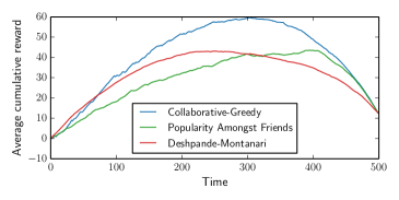
(b)

Figure 1: Movielens10m dataset: (a) Top users by top movies matrix with rows and columns reordered to show clustering of users and items. (b) Average cumulative rewards over time.

6 Discussion and Related Work

This paper proposes a model for online recommendation systems under which we can analyze the performance of recommendation algorithms. We theoretical justify when a cosine-similarity collaborative filtering method works well, with a key insight of using two exploration types.

The closest related work is by Biau et al. [7], who study the asymptotic consistency of a cosine-similarity nearest-neighbor collaborative filtering method. Their goal is to predict the rating of the next unseen item. Barman and Dabeer [4] study the performance of an algorithm called Popularity Amongst Friends, examining its ability to predict binary ratings in an asymptotic information-theoretic setting. In contrast, we seek to understand the finite-time performance of such systems. Dabeer [11] uses a model similar to ours and studies online collaborative filtering with a moving horizon cost in the limit of small noise using an algorithm that knows the numbers of user types and item types. We do not model different item types, our algorithm is oblivious to the number of user types, and our performance metric is different. Another related work is by Deshpande and Montanari [12], who study online recommendations as a linear bandit problem; their method, however, does not actually use any collaboration beyond a pre-processing step in which offline collaborative filtering (specifically matrix completion) is solved to compute feature vectors for items.

Our work also relates to the problem of learning mixture distributions (c.f., [10, 18, 5, 2]), where one observes samples from a mixture distribution and the goal is to learn the mixture components and weights. Existing results assume that one has access to the entire high-dimensional sample or that the samples are produced in an exogenous manner (not chosen by the algorithm). Neither assumption holds in our setting, as we only see each user’s revealed ratings thus far and not the user’s entire preference vector, and the recommendation algorithm affects which samples are observed (by choosing which item ratings are revealed for each user). These two aspects make our setting more challenging than the standard setting for learning mixture distributions. However, our goal is more modest. Rather than learning the $k$ item preference vectors, we settle for classifying them as likable or unlikable. Despite this, we suspect having two types of exploration to be useful in general for efficiently learning mixture distributions in the active learning setting.

Acknowledgements. This work was supported in part by NSF grant CNS-1161964 and by Army Research Office MURI Award W911NF-11-1-0036. GHC was supported by an NDSEG fellowship.

Appendix A Appendix

Throughout our derivations, if it is clear from context, we omit the argument $(t)$ indexing time, for example writing $Y_{u}$ instead of $Y_{u}(t)$.

A.1 Proof of Lemma 1

We reproduce Lemma 1 below for ease of presentation.

Lemma 1.

For user $u$, after

$$t\geq\bigg{(}\frac{2\log(10kmn^{\alpha}/\Delta)}{\Delta^{4}(1-\gamma)^{2}}\bigg{)}^{1/(1-\alpha)}$$

time steps,

$$\mathbb{P}(\mathcal{E}_{\text{good}}(u,t)) \geq 1-\exp\Big{(}-\frac{n}{8k}\Big{)}-12\exp\Big{(}-\frac{\Delta^{4}(1-\gamma)^{2}t^{1-\alpha}}{20}\Big{)}\,.$$

To derive this lower bound on the probability that the good neighborhood event $\mathcal{E}_{\text{good}}(u,t)$ occurs, we prove four lemmas (Lemmas 4, 5, 6, and 7). Before doing so, we define a constant that will appear several times:

$$\beta\triangleq\exp(-\Delta^{4}(1-\gamma)^{2}t^{1-\alpha}).$$

We begin by ensuring that enough users from each of the $k$ user types are in the system.

Lemma 4.

For a user $u$,

$$\mathbb{P}\Big{(}\text{user $u$'s type has}\leq\frac{n}{2k}\text{ users}\Big{)}\leq\exp\Big{(}-\frac{n}{8k}\Big{)}.$$

Proof.

Let $N$ be the number of users from user $u$’s type. User types are equiprobable, so $N\sim\text{Bin}(n,\frac{1}{k})$. By a Chernoff bound,

$$\mathbb{P}\Big{(}N\leq\frac{n}{2k}\Big{)}\leq\exp\bigg{(}-\frac{1}{2}\frac{(\frac{n}{k}-\frac{n}{2k})^{2}}{\frac{n}{k}}\bigg{)}=\exp\Big{(}-\frac{n}{8k}\Big{)}.\qed$$

Next, we ensure that sufficiently many items have been jointly explored across all users. This will subsequently be used for bounding both the number of good neighbors and the number of bad neighbors.

Lemma 5.

After $t$ time steps,

$$\mathbb{P}(\text{fewer than }t^{1-\alpha}/2\text{ jointly explored items}) \leq\exp(-t^{1-\alpha}/20).$$

Proof.

Let $Z_{s}$ be the indicator random variable for the event that the algorithm jointly explores at time $s$. Thus, the number of jointly explored items up to time $t$ is $\sum_{s=1}^{t}Z_{s}$. By our choice for the time-varying joint exploration probability $\varepsilon_{J}$, we have $\mathbb{P}(Z_{s}=1)=\varepsilon_{J}(s)=\frac{1}{s^{\alpha}}$ and $\mathbb{P}(Z_{s}=0)=1-\frac{1}{s^{\alpha}}$. Note that the centered random variable $\bar{Z}_{s}=\mathbb{E}[Z_{s}]-Z_{s}=\frac{1}{s^{\alpha}}-Z_{s}$ has zero mean, and $|\bar{Z}_{s}|\leq 1$ with probability 1. Then,

$$\mathbb{P}\bigg{(}\sum_{s=1}^{t}Z_{s}<\frac{1}{2}t^{1-\alpha}\bigg{)} =\mathbb{P}\bigg{(}\sum_{s=1}^{t}\bar{Z}_{s}>\sum_{s=1}^{t}\mathbb{E}[Z_{s}]-\frac{1}{2}t^{1-\alpha}\bigg{)}\overset{(i)}{\leq}\mathbb{P}\bigg{(}\sum_{s=1}^{t}\bar{Z}_{s}>\frac{1}{2}t^{1-\alpha}\bigg{)}$$

$$\overset{(ii)}{\leq}\exp\bigg{(}-\frac{\frac{1}{8}t^{2(1-\alpha)}}{\sum_{s=1}^{t}\mathbb{E}[\bar{Z}_{s}^{2}]+\frac{1}{6}t^{1-\alpha}}\bigg{)}\overset{(iii)}{\leq}\exp\bigg{(}-\frac{\frac{1}{8}t^{2(1-\alpha)}}{\frac{t^{1-\alpha}}{1-\alpha}+\frac{1}{6}t^{1-\alpha}}\bigg{)}$$

$$=\exp\bigg{(}-\frac{3(1-\alpha)t^{1-\alpha}}{4(7-\alpha)}\bigg{)}\overset{(iv)}{\leq}\exp(-t^{1-\alpha}/20),$$

where step $(i)$ uses the fact that $\sum_{s=1}^{t}\mathbb{E}[Z_{s}]=\sum_{s=1}^{t}1/s^{\alpha}\geq t/t^{\alpha}=t^{1-\alpha}$, step $(ii)$ is Bernstein’s inequality, step $(iii)$ uses the fact that $\sum_{s=1}^{t}\mathbb{E}[\bar{Z}_{s}^{2}]\leq\sum_{s=1}^{t}\mathbb{E}[Z_{s}^{2}]=\sum_{s=1}^{t}1/s^{\alpha}\leq t^{1-\alpha}/(1-\alpha)$, and step $(iv)$ uses the fact that $\alpha\leq 4/7$. (We remark that the choice of constant $4/7$ isn’t special; changing it would simply modify the constant in the decaying exponentially to potentially no longer be $1/20$). ∎

Assuming that the bad events for the previous two lemmas do not occur, we now provide a lower bound on the number of good neighbors that holds with high probability.

Lemma 6.

Suppose that there are no $\Delta$-ambiguous items, that there are more than $\frac{n}{2k}$ users of user $u$’s type, and that all users have rated at least $t^{1-\alpha}/2$ items as part of joint exploration. For user $u$, let $n_{\text{good}}$ be the number of “good” neighbors of user $u$. If $\beta\leq\frac{1}{10}$, then

$$\mathbb{P}\Big{(}n_{\text{good}}\leq(1-\beta)\frac{n}{4k}\Big{)}\leq 10\beta.$$

We defer the proof of Lemma 6 to Appendix A.1.1.

Finally, we verify that the number of bad neighbors for any user is not too large, again conditioned on there being enough jointly explored items.

Lemma 7.

Suppose that the minimum number of rated items in common between any pair of users is $t^{1-\alpha}/2$ and suppose that $\gamma$-incoherence holds for some $\gamma\in[0,1)$. For user $u$, let $n_{\text{bad}}$ be the number of “bad” neighbors of user $u$. Then

$$\mathbb{P}(n_{\text{bad}}\geq n\sqrt{\beta})\leq\sqrt{\beta}.$$

We defer the proof of Lemma 7 to Appendix A.1.2.

We now prove Lemma 1, which union bounds over the four bad events of Lemmas 4, 5, 6, and 7. Recall that the good neighborhood event $\mathcal{E}_{\text{good}}(u,t)$ holds if at time $t$, user $u$ has more than $\frac{n}{5k}$ good neighbors and less than $\frac{\Delta tn^{1-\alpha}}{10km}$ bad neighbors. By assuming that the four bad events don’t happen, then Lemma 6 tells us that there are more than $(1-\beta)\frac{n}{4k}$ good neighbors provided that $\beta\leq\frac{1}{10}$. Thus, to ensure that there are more than $\frac{n}{5k}$ good neighbors, it suffices to have $(1-\beta)\frac{n}{4k}\geq\frac{n}{5k}$, which happens when $\beta\leq\frac{1}{5}$, but we already require that $\beta\leq\frac{1}{10}$. Similarly, Lemma 7 tells us that there are fewer than $n\sqrt{\beta}$ bad neighbors, so to ensure that there are fewer than $\frac{\Delta tn^{1-\alpha}}{10km}$ bad neighbors it suffices to have $n\sqrt{\beta}\leq\frac{\Delta tn^{1-\alpha}}{10km}$, which happens when $\beta\leq(\frac{\Delta t}{10kmn^{\alpha}})^{2}$. We can satisfy all constraints on $\beta$ by asking that $\beta\leq(\frac{\Delta}{10kmn^{\alpha}})^{2}$, which is tantamount to asking that

$$t\geq\bigg{(}\frac{2\log(10kmn^{\alpha}/\Delta)}{\Delta^{4}(1-\gamma)^{2}}\bigg{)}^{1/(1-\alpha)}$$

since $\beta=\exp(-\Delta^{4}(1-\gamma)^{2}t^{1-\alpha})$.

Finally, with $t$ satisfying the inequality above, the union bound over the four bad events can be further bounded to complete the proof:

$$\mathbb{P}(\mathcal{E}_{\text{good}}(u,t)) \geq 1-\exp\Big{(}-\frac{n}{8k}\Big{)}-\exp(-t^{1-\alpha}/20)-10\beta-\sqrt{\beta}$$

$$\geq 1-\exp\Big{(}-\frac{n}{8k}\Big{)}-12\exp\Big{(}-\frac{\Delta^{4}(1-\gamma)^{2}t^{1-\alpha}}{20}\Big{)}.$$

A.1.1 Proof of Lemma 6

We begin with a preliminary lemma that upper-bounds the probability of two users of the same type not being declared as neighbors.

Lemma 8.

Suppose that there are no $\Delta$-ambiguous items for any of the user types. Let users $u$ and $v$ be of the same type, and suppose that they have rated at least $\Gamma_{0}$ items in common (explored jointly). Then for $\theta\in(0,4\Delta^{2})$,

$$\mathbb{P}(\text{users }u\text{ and }v\text{ are not declared as neighbors})\leq\exp\Big{(}-\frac{(4\Delta^{2}-\theta)^{2}}{2}\Gamma_{0}\Big{)}.$$

Proof.

Let us first suppose that users $u$ and $v$ have rated exactly $\Gamma_{0}$ items in common. The two users are not declared to be neighbors if $\langle\widetilde{Y}_{u},\widetilde{Y}_{v}\rangle<\theta\Gamma_{0}$. Let $\Omega\subseteq[m]$ such that $|\Omega|=\Gamma_{0}$. We have

$$\mathbb{E}\big{[}\langle\widetilde{Y}_{u},\widetilde{Y}_{v}\rangle\big{|}\text{supp}(\widetilde{Y}_{u})\cap\text{supp}(\widetilde{Y}_{v})=\Omega\big{]} =\sum_{i\in\Omega}\mathbb{E}[\widetilde{Y}_{ui}\widetilde{Y}_{vi}\mid\widetilde{Y}_{ui}\neq 0,\widetilde{Y}_{vi}\neq 0]$$

$$=\sum_{i\in\Omega}(p_{ui}^{2}+(1-p_{ui})^{2}-2p_{ui}(1-p_{ui}))$$

$$=4\sum_{i\in\Omega}\Big{(}p_{ui}-\frac{1}{2}\Big{)}^{2}.$$ (2)

Since $\langle\widetilde{Y}_{u},\widetilde{Y}_{v}\rangle=\sum_{i\in\Omega}\widetilde{Y}_{ui}\widetilde{Y}_{vi}$ is the sum of terms $\{\widetilde{Y}_{ui}\widetilde{Y}_{vi}\}_{i\in\Omega}$ that are each bounded within $[-1,1]$, Hoeffding’s inequality yields

$$\mathbb{P}\big{(}\langle\widetilde{Y}_{u},\widetilde{Y}_{v}\rangle\leq\theta\Gamma_{0}\;\big{|}\;\text{supp}(\widetilde{Y}_{u})\cap\text{supp}(\widetilde{Y}_{v})=\Omega\big{)}\leq\exp\bigg{(}-\frac{\big{[}\overbrace{4\textstyle{\sum_{i\in\Omega}}\big{(}p_{gi}-\frac{1}{2}\big{)}^{2}}^{\text{equation\,}\eqref{eq:same-source-E-inner-prod}}-\theta\Gamma_{0}\big{]}^{2}}{2\Gamma_{0}}\bigg{)}.$$ (3)

As there are no $\Delta$-ambiguous items, $\Delta\leq|p_{ui}-1/2|$ for all users $u$ and items $i$. Thus, our choice of $\theta$ guarantees that

$$4\sum_{i\in\Omega}\Big{(}p_{ui}-\frac{1}{2}\Big{)}^{2}-\theta\Gamma_{0}\geq 4\Gamma_{0}\Delta^{2}-\theta\Gamma_{0}=(4\Delta^{2}-\theta)\Gamma_{0}\geq 0.$$ (4)

Combining inequalities (3) and (4), and observing that the above holds for all subsets $\Omega$ of cardinality $\Gamma_{0}$, we obtain the desired bound on the probability that users $u$ and $v$ are not declared as neighbors:

$$\mathbb{P}(\langle\widetilde{Y}_{u},\widetilde{Y}_{v}\rangle\leq\theta\Gamma_{0}\;|\;|\text{supp}(\widetilde{Y}_{u})\cap\text{supp}(\widetilde{Y}_{v})|=\Gamma_{0})\leq\exp\Big{(}-\frac{(4\Delta^{2}-\theta)^{2}}{2}\Gamma_{0}\Big{)}.$$ (5)

Now to handle the case that users $u$ and $v$ have jointly rated more than $\Gamma_{0}$ items, observe that, with shorthand $\Gamma_{uv}\triangleq|\text{supp}(\widetilde{Y}_{u})\cap\text{supp}(\widetilde{Y}_{v})|$,

$$\mathbb{P}(u\text{ and }v\text{ not declared neighbors}\,|\,p_{u}=p_{v},\Gamma_{uv}\geq\Gamma_{0})$$

$$=\mathbb{P}(\langle\widetilde{Y}_{u},\widetilde{Y}_{v}\rangle<\theta\Gamma_{uv}\;|\;p_{u}=p_{v},\;\Gamma_{uv}\geq\Gamma_{0})$$

$$=\frac{\mathbb{P}(\langle\widetilde{Y}_{u},\widetilde{Y}_{v}\rangle\leq\theta\Gamma_{uv},\Gamma_{uv}\geq\Gamma_{0}\;|\;p_{u}=p_{v})}{\mathbb{P}(\Gamma_{uv}\geq\Gamma_{0}\;|\;p_{u}=p_{v})}$$

$$=\frac{\sum_{\ell=\Gamma_{0}}^{m}\mathbb{P}(\langle\widetilde{Y}_{u},\widetilde{Y}_{v}\rangle\leq\theta\ell,\Gamma_{uv}=\ell\;|\;p_{u}=p_{v})}{\mathbb{P}(\Gamma_{uv}\geq\Gamma_{0}\;|\;p_{u}=p_{v})}$$

$$=\frac{\sum_{\ell=\Gamma_{0}}^{m}\begin{array}[]{c}\big{[}\mathbb{P}(\Gamma_{uv}=\ell\;|\;p_{u}=p_{v})\\ \cdot\mathbb{P}(\langle\widetilde{Y}_{u},\widetilde{Y}_{v}\rangle\leq\theta\ell\;|\;p_{u}=p_{v},\Gamma_{uv}=\ell)\big{]}\end{array}}{\mathbb{P}(\Gamma_{uv}\geq\Gamma_{0}\;|\;p_{u}=p_{v})}$$

$$\leq\frac{\sum_{\ell=\Gamma_{0}}^{m}\mathbb{P}(\Gamma_{uv}=\ell\;|\;p_{u}=p_{v})\exp\big{(}-\frac{(4\Delta^{2}-\theta)^{2}}{2}\Gamma_{0}\big{)}}{\mathbb{P}(\Gamma_{uv}\geq\Gamma_{0}\;|\;p_{u}=p_{v})}$$

$$\quad\;\;\text{by inequality }\eqref{eq:same-source-prob-error-exact-overlap-amount}$$

$$=\exp\Big{(}-\frac{(4\Delta^{2}-\theta)^{2}}{2}\Gamma_{0}\Big{)}.\qed$$

We now prove Lemma 6.

Suppose that the event in Lemma 4 holds. Let $\mathcal{G}$ be $\frac{n}{2k}$ users from the same user type as user $u$; there could be more than $\frac{n}{2k}$ such users but it suffices to consider $\frac{n}{2k}$ of them. We define an indicator random variable

$$G_{v}\triangleq\mathds{1}\{\text{users }u\text{ and }v\text{ are neighbors}\}=\mathds{1}\{\langle\widetilde{Y}_{u}^{(t)},\widetilde{Y}_{v}^{(t)}\rangle\geq\theta t^{1-\alpha}/2\}.$$

Thus, the number of good neighbors of user $u$ is lower-bounded by $W=\sum_{v\in\mathcal{G}}G_{v}$. Note that the $G_{v}$’s are not independent. To arrive at a lower bound for $W$ that holds with high probability, we use Chebyshev’s inequality:

$$\mathbb{P}(W-\mathbb{E}[W]\leq-\mathbb{E}[W]/2)\leq\frac{4\mathrm{Var}(W)}{(\mathbb{E}[W])^{2}}\,.$$ (6)

Let $\beta=\exp(-(4\Delta^{2}-\theta)^{2}\Gamma_{0}/2)$ be the probability bound from Lemma 8, where by our choice of $\theta=2\Delta^{2}(1+\gamma)$ and with $\Gamma_{0}=t^{1-\alpha}/2$, we have $\beta=\exp(-\Delta^{4}(1-\gamma)^{2}t^{1-\alpha})$.

Applying Lemma 8, we have $\mathbb{E}[W]\geq(1-\beta)\frac{n}{2k}$, and hence

$$(\mathbb{E}[W])^{2}\geq(1-2\beta)\frac{n^{2}}{4k^{2}}.$$ (7)

We now upper-bound

$$\text{Var}(W)=\sum_{v\in\mathcal{G}}\text{Var}(G_{v})+\sum_{v\neq w}\text{Cov}(G_{v},G_{w}).$$

Since $G_{v}=G_{v}^{2}$,

$$\text{Var}(G_{v})=\mathbb{E}[G_{v}]-\mathbb{E}[G_{v}]^{2}=\underbrace{\mathbb{E}[G_{v}]}_{\leq 1}(1-\mathbb{E}[G_{v}])\leq\beta,$$

where the last step uses Lemma 8.

Meanwhile,

$$\text{Cov}(G_{v},G_{w})=\mathbb{E}[G_{v}G_{w}]-\mathbb{E}[G_{v}]\mathbb{E}[G_{w}]\leq 1-(1-\beta)^{2}\leq 2\beta.$$

Putting together the pieces,

$$\text{Var}(W)\leq\frac{n}{2k}\cdot\beta+\frac{n}{2k}\cdot\Big{(}\frac{n}{2k}-1\Big{)}\cdot 2\beta\leq\frac{n^{2}}{2k^{2}}\cdot\beta.$$ (8)

Plugging (7) and (8) into (6) gives

$$\mathbb{P}(W-\mathbb{E}[W]\leq-\mathbb{E}[W]/2)\leq\frac{8\beta}{1-2\beta}\leq 10\beta,$$

provided that $\beta\leq\frac{1}{10}$. Thus, $n_{\text{good}}\geq W\geq\mathbb{E}[W]/2\geq(1-\beta)\frac{n}{4k}$ with probability at least $1-10\beta$.

A.1.2 Proof of Lemma 7

We begin with a preliminary lemma that upper-bounds the probability of two users of different types being declared as neighbors.

Lemma 9.

Let users $u$ and $v$ be of different types, and suppose that they have rated at least $\Gamma_{0}$ items in common via joint exploration. Further suppose $\gamma$-incoherence is satisfied for $\gamma\in[0,1)$. If $\theta\geq 4\gamma\Delta^{2}$, then

$$\mathbb{P}(\text{users }u\text{ and }v\text{ are declared to be neighbors})\leq\exp\Big{(}-\frac{(\theta-4\gamma\Delta^{2})^{2}}{2}\Gamma_{0}\Big{)}.$$

Proof.

As with the proof of Lemma 8, we first analyze the case where users $u$ and $v$ have rated exactly $\Gamma_{0}$ items in common. Users $u$ and $v$ are declared to be neighbors if $\langle\widetilde{Y}_{u},\widetilde{Y}_{v}\rangle\geq\theta\Gamma_{0}$. We now crucially use the fact that joint exploration chooses these $\Gamma_{0}$ items as a random subset of the $m$ items. For our random permutation $\sigma$ of $m$ items, we have $\langle\widetilde{Y}_{u},\widetilde{Y}_{v}\rangle=\sum_{i=1}^{\Gamma_{0}}\widetilde{Y}_{u,\sigma(i)}\widetilde{Y}_{v,\sigma(i)}=\sum_{i=1}^{\Gamma_{0}}Y_{u,\sigma(i)}Y_{v,\sigma(i)}$, which is the sum of terms $\{Y_{u,\sigma(i)}Y_{v,\sigma(i)}\}_{i=1}^{\Gamma_{0}}$ that are each bounded within $[-1,1]$ and drawn without replacement from a population of all possible items. Hoeffding’s inequality (which also applies to the current scenario of sampling without replacement [14]) yields

$$\mathbb{P}\big{(}\langle\widetilde{Y}_{u},\widetilde{Y}_{v}\rangle\geq\theta\Gamma_{0}\mid p_{u}\neq p_{v}\big{)}\leq\exp\left(-\frac{\big{(}\theta\Gamma_{0}-\mathbb{E}[\langle\widetilde{Y}_{u},\widetilde{Y}_{v}\rangle\mid p_{u}\neq p_{v}]\big{)}^{2}}{2\Gamma_{0}}\right).$$ (9)

By $\gamma$-incoherence and our choice of $\theta$,

$$\theta\Gamma_{0}-\mathbb{E}\big{[}\langle\widetilde{Y}_{u},\widetilde{Y}_{v}\rangle\mid p_{u}\neq p_{v}\big{]}\geq\theta\Gamma_{0}-4\gamma\Delta^{2}\Gamma_{0}=(\theta-4\gamma\Delta^{2})\Gamma_{0}\geq 0.$$ (10)

Above, we used the fact that $\Gamma_{0}$ randomly explored items are a random subset of $m$ items, and hence

$$\mathbb{E}\big{[}\tfrac{1}{\Gamma}_{0}\langle\widetilde{Y}_{u},\widetilde{Y}_{v}\rangle\big{]} =\mathbb{E}\big{[}\tfrac{1}{m}\langle{Y}_{u},{Y}_{v}\rangle\big{]},$$

with $Y_{u},Y_{v}$ representing the entire (random) vector of preferences of $u$ and $v$ respectively.

Combining inequalities (9) and (10) yields

$$\mathbb{P}\big{(}\langle\widetilde{Y}_{u},\widetilde{Y}_{v}\rangle\geq\theta\Gamma_{0}\mid p_{u}\neq p_{v}\big{)}\leq\exp\Big{(}-\frac{(\theta-4\gamma\Delta^{2})^{2}}{2}\Gamma_{0}\Big{)}.$$

A similar argument as the ending of Lemma 8’s proof establishes that the bound holds even if users $u$ and $v$ have jointly explored more than $\Gamma_{0}$ items. ∎

We now prove Lemma 7.

Let $\beta=\exp(-(\theta-4\gamma\Delta^{2})^{2}\Gamma_{0}/2)$ be the probability bound from Lemma 9, where by our choice of $\theta=2\Delta^{2}(1+\gamma)$ and with $\Gamma_{0}=t^{1-\alpha}/2$, we have $\beta=\exp(-\Delta^{4}(1-\gamma)^{2}t^{1-\alpha})$.

By Lemma 9, for a pair of users $u$ and $v$ with at least $t^{1-\alpha}/2$ items jointly explored, the probability that they are erroneously declared neighbors is upper-bounded by $\beta$.

Denote the set of users of type different from $u$ by $\mathcal{B}$, and write

$$n_{\text{bad}}=\sum_{v\in\mathcal{B}}\mathds{1}\{u\text{ and }v\text{ are declared to be neighbors}\},$$

whence $\mathbb{E}[n_{\text{bad}}]\leq n\beta$. Markov’s inequality gives

$$\mathbb{P}(n_{\text{bad}}\geq n\sqrt{\beta})\leq\frac{\mathbb{E}[n_{\text{bad}}]}{n\sqrt{\beta}}\leq\frac{n\beta}{n\sqrt{\beta}}=\sqrt{\beta}\,,$$

proving the lemma.

A.2 Proof of Lemma 2

We reproduce Lemma 2 below.

Lemma 2.

For user $u$ at time $t$, if the good neighborhood event $\mathcal{E}_{\text{good}}(u,t)$ holds and $t\leq\mu m$, then

$$\mathbb{P}(X_{ut}=1) \geq 1-2m\exp\Big{(}-\frac{\Delta^{2}tn^{1-\alpha}}{40km}\Big{)}-\frac{1}{t^{\alpha}}-\frac{1}{n^{\alpha}}\,.$$

We begin by checking that when the good neighborhood event $\mathcal{E}_{\text{good}}(u,t)$ holds for user $u$, the items have been rated enough times by the good neighbors.

Lemma 10.

For user $u$ at time $t$, suppose that the good neighborhood event $\mathcal{E}_{\text{good}}(u,t)$ holds. Then for a given item $i$,

$$\mathbb{P}\Big{(}\text{item }i\text{ has}\leq\frac{tn^{1-\alpha}}{10km}\text{ ratings from good neighbors of }u\Big{)}\leq\exp\Big{(}-\frac{tn^{1-\alpha}}{40km}\Big{)}.$$

Proof.

The number of user $u$’s good neighbors who have rated item $i$ stochastically dominates a $\text{Bin}(\frac{n}{5k},\frac{\varepsilon_{R}(n)t}{m})$ random variable, where $\frac{\varepsilon_{R}(n)t}{m}=\frac{t}{mn^{\alpha}}$ (here, we have critically used the lower bound on the number of good neighbors user $u$ has when the good neighborhood event $\mathcal{E}_{\text{good}}(u,t)$ holds). By a Chernoff bound,

$$\mathbb{P}\bigg{(}\text{Bin}\Big{(}\frac{n}{5k},\frac{t}{mn^{\alpha}}\Big{)}\leq\frac{tn^{1-\alpha}}{10km}\bigg{)}\leq\exp\bigg{(}-\frac{1}{2}\frac{(\frac{tn^{1-\alpha}}{5km}-\frac{tn^{1-\alpha}}{10km})^{2}}{\frac{tn^{1-\alpha}}{5km}}\bigg{)}\leq\exp\Big{(}-\frac{tn^{1-\alpha}}{40km}\Big{)}.\qed$$

Next, we show a sufficient condition for which the algorithm correctly classifies every item as likable or unlikable for user $u$.

Lemma 11.

Suppose that there are no $\Delta$-ambiguous items. For user $u$ at time $t$, suppose that the good neighborhood event $\mathcal{E}_{\text{good}}(u,t)$ holds. Provided that every item $i\in[m]$ has more than $\frac{tn^{1-\alpha}}{10km}$ ratings from good neighbors of user $u$, then with probability at least $1-m\exp(-\frac{\Delta^{2}tn^{1-\alpha}}{20km})$, we have that for every item $i\in[m]$,

$$\widetilde{p}_{ui} >\frac{1}{2}\quad\text{if item }i\text{ is likable by user }u,$$

$$\widetilde{p}_{ui} <\frac{1}{2}\quad\text{if item }i\text{ is unlikable by user }u.$$

Proof.

Let $A$ be the number of ratings that good neighbors of user $u$ have provided. Suppose item $i$ is likable by user $u$. Then when we condition on $A=a_{0}\triangleq\lceil\frac{tn^{1-\alpha}}{10km}\rceil$, $\widetilde{p}_{ui}$ stochastically dominates

$$q_{ui}\triangleq\frac{\text{Bin}(a_{0},p_{ui})}{a_{0}+\Delta a_{0}}=\frac{\text{Bin}(a_{0},p_{ui})}{(1+\Delta)a_{0}},$$

which is the worst-case variant of $\widetilde{p}_{ui}$ that insists that all $\Delta a_{0}$ bad neighbors provided rating “$-1$” for likable item $i$ (here, we have critically used the upper bound on the number of bad neighbors user $u$ has when the good neighborhood event $\mathcal{E}_{\text{good}}(u,t)$ holds). Then

$$\mathbb{P}(q_{ui}\leq\frac{1}{2}\mid A=a_{0}) =\mathbb{P}\bigg{(}\text{Bin}(a_{0},p_{ui})\leq\frac{(1+\Delta)a_{0}}{2}\;\bigg{|}\;A=a_{0}\bigg{)}$$

$$=\mathbb{P}\bigg{(}a_{0}p_{ui}-\text{Bin}(a_{0},p_{ui})\geq a_{0}\Big{(}p_{ui}-\frac{1}{2}-\frac{\Delta}{2}\Big{)}\;\bigg{|}\;A=a_{0}\bigg{)}$$

$$\overset{(i)}{\leq}\exp\Big{(}-2a_{0}\Big{(}p_{ui}-\frac{1}{2}-\frac{\Delta}{2}\Big{)}^{2}\Big{)}$$

$$\overset{(ii)}{\leq}\exp\Big{(}-\frac{1}{2}a_{0}\Delta^{2}\Big{)}$$

$$\overset{(iii)}{\leq}\exp\Big{(}-\frac{\Delta^{2}tn^{1-\alpha}}{20km}\Big{)},$$

where step $(i)$ is Hoeffding’s inequality, step $(ii)$ follows from item $i$ being likable by user $u$ (i.e., $p_{ui}\geq\frac{1}{2}+\Delta$), and step $(iii)$ is by our choice of $a_{0}$. Conclude then that

$$\mathbb{P}(\widetilde{p}_{ui}\leq\frac{1}{2}\mid A=a_{0})\leq\exp\Big{(}-\frac{\Delta^{2}tn^{1-\alpha}}{20km}\Big{)}.$$

Finally,

$$\mathbb{P}\Big{(}\widetilde{p}_{ui}\leq\frac{1}{2}\;\Big{|}\;A\geq\frac{tn^{1-\alpha}}{10km}\Big{)} =\frac{\sum_{a=a_{0}}^{\infty}\mathbb{P}(A=a)\mathbb{P}(\widetilde{p}_{ui}\leq\frac{1}{2}\mid A=a)}{\mathbb{P}(A\geq\frac{tn^{1-\alpha}}{10km})}$$

$$\leq\frac{\sum_{a=a_{0}}^{\infty}\mathbb{P}(A=a)\exp(-\frac{\Delta^{2}tn^{1-\alpha}}{20km})}{\mathbb{P}(A\geq\frac{tn^{1-\alpha}}{10km})}$$

$$=\exp\Big{(}-\frac{\Delta^{2}tn^{1-\alpha}}{20km}\Big{)}.$$

A similar argument holds for when item $i$ is unlikable. Union-bounding over all $m$ items yields the claim. ∎

We now prove Lemma 2. First off, provided that $t\leq\mu m$, we know that there must still exist an item likable by user $u$ that user $u$ has yet to consume. For user $u$ at time $t$, supposing that event $\mathcal{E}_{\text{good}}(u,t)$ holds, then every item has been rated more than $\frac{tn^{1-\alpha}}{10km}$ times by the good neighbors of user $u$ with probability at least $1-m\exp(-\frac{tn^{1-\alpha}}{40km})$. This follows from union-bounding over the $m$ items with Lemma 10. Applying Lemma 11, and noting that we only exploit with probability $1-\varepsilon_{J}(t)-\varepsilon_{R}(n)=1-1/t^{\alpha}-1/n^{\alpha}$, we finish the proof:

$$\mathbb{P}(X_{ut}=1) \geq 1-m\exp\Big{(}-\frac{tn^{1-\alpha}}{40km}\Big{)}-m\exp\Big{(}-\frac{\Delta^{2}tn^{1-\alpha}}{20km}\Big{)}-\frac{1}{t^{\alpha}}-\frac{1}{n^{\alpha}}$$

$$\geq 1-2m\exp\Big{(}-\frac{\Delta^{2}tn^{1-\alpha}}{40km}\Big{)}-\frac{1}{t^{\alpha}}-\frac{1}{n^{\alpha}}.$$

A.3 Experimental Results

We demonstrate our algorithm Collaborative-Greedy on two datasets, showing that they have comparable performance and that they both outperform two existing recommendation algorithms Popularity Amongst Friends (PAF) [4] and Deshpande and Montanari’s method (DM) [12]. At each time step, PAF finds nearest neighbors (“friends”) for every user and recommends to a user the “most popular” item, i.e., the one with the most number of $+1$ ratings, among the user’s friends. DM doesn’t do any collaboration beyond a preprocessing step that computes item feature vectors via matrix completion. Then during online recommendation, DM learns user feature vectors over time with the help of item feature vectors and recommends an item to each user based on whether it aligns well with the user’s feature vector.

We simulate an online recommendation system based on movie ratings from the Movielens10m and Netflix datasets, each of which provides a sparsely filled user-by-movie rating matrix with ratings out of 5 stars. Unfortunately, existing collaborative filtering datasets such as the two we consider don’t offer the interactivity of a real online recommendation system, nor do they allow us to reveal the rating for an item that a user didn’t actually rate. For simulating an online system, the former issue can be dealt with by simply revealing entries in the user-by-item rating matrix over time. We address the latter issue by only considering a dense “top users vs. top items” subset of each dataset. In particular, we consider only the “top” users who have rated the most number of items, and the “top” items that have received the most number of ratings. While this dense part of the dataset is unrepresentative of the rest of the dataset, it does allow us to use actual ratings provided by users without synthesizing any ratings.

An initial question to ask is whether the dense movie ratings matrices we consider could be reasonably explained by our latent source model. We automatically learn the structure of these matrices using the method by Grosse et al. [13] and find Bayesian clustered tensor factorization (BCTF) to accurately model the data. This finding isn’t surprising as BCTF has previously been used to model movie ratings data [21]. BCTF effectively clusters both users and movies so that we get structure such as that shown in Figure 1LABEL:sub@fig:bctf for the Movielens10m “top users vs. top items” matrix. Our latent source model could reasonably model movie ratings data as it only assumes clustering of users.

Following the experimental setup of [4], we quantize a rating of 4 stars or more to be $+1$ (likeable), and a rating of 3 stars or less to be $-1$ (unlikeable). While we look at a dense subset of each dataset, there are still missing entries. If a user $u$ hasn’t rated item $j$ in the dataset, then we set the corresponding true rating to 0, meaning that in our simulation, upon recommending item $j$ to user $u$, we receive 0 reward, but we still mark that user $u$ has consumed item $j$; thus, item $j$ can no longer be recommended to user $u$. For both Movielens10m and Netflix datasets, we consider the top $n=200$ users and the top $m=500$ movies. For Movielens10m, the resulting user-by-rating matrix has 80.7% nonzero entries. For Netflix, the resulting matrix has 86.0% nonzero entries. For an algorithm that recommends item $\pi_{ut}$ to user $u$ at time $t$, we measure the algorithm’s average cumulative reward up to time $T$ as

$$\frac{1}{n}\sum_{t=1}^{T}\sum_{u=1}^{n}Y_{u\pi_{ut}}^{(T)},$$

where we average over users.

For all methods, we recommend items until we reach time $T=500$, i.e., we make movie recommendations until each user has seen all $m=500$ movies. We disallow the matrix completion step for DM to see the users that we actually test on, but we allow it to see the the same items as what is in the simulated online recommendation system in order to compute these items’ feature vectors (using the rest of the users in the dataset). Furthermore, when a rating is revealed, we provide DM both the thresholded rating and the non-thresholded rating, the latter of which DM uses to estimate user feature vectors over time.

Parameters $\theta$ and $\alpha$ for and Collaborative-Greedy are chosen using training data: We sweep over the two parameters on training data consisting of 200 users that are the “next top” 200 users, i.e., ranked 201 to 400 in number movie ratings they provided. For simplicity, we discretize our search space to $\theta\in\{0.0,0.1,\dots,1.0\}$ and $\alpha\in\{0.1,0.2,0.3,0.4,0.5\}$. We choose the parameter setting achieving the highest area under the cumulative reward curve. For both Movielens10m and Netflix datasets, this corresponded to setting $\theta=0.0$ and $\alpha=0.5$ for Collaborative-Greedy. In contrast, the parameters for PAF and DM are chosen to be the best parameters for the test data among a wide range of parameters. The results are shown in Figure 2. We find that our algorithm Collaborative-Greedy outperforms PAF and DM. We remark that the curves are roughly concave, which is expected since once we’ve finished recommending likeable items (roughly around time step 300), we end up recommending mostly unlikeable items until we’ve exhausted all the items.

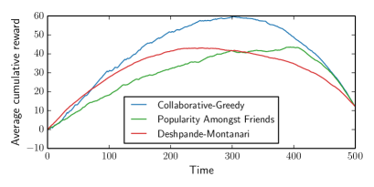
(a)

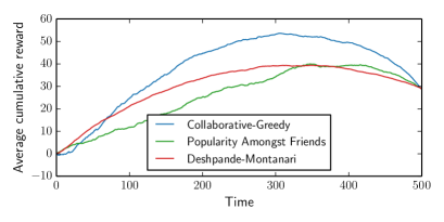
(b)

Figure 2: Average cumulative rewards over time: (a) Movielens10m, (b) Netflix.

References

- [1] Fabio Aiolli. A preliminary study on a recommender system for the million songs dataset challenge. In Proceedings of the Italian Information Retrieval Workshop, pages 73–83, 2013.
- [2] Anima Anandkumar, Rong Ge, Daniel Hsu, Sham M. Kakade, and Matus Telgarsky. Tensor decompositions for learning latent variable models, 2012. arXiv:1210.7559.
- [3] Peter Auer, Nicolò Cesa-Bianchi, and Paul Fischer. Finite-time analysis of the multiarmed bandit problem. Machine Learning, 47(2-3):235–256, May 2002.
- [4] Kishor Barman and Onkar Dabeer. Analysis of a collaborative filter based on popularity amongst neighbors. IEEE Transactions on Information Theory, 58(12):7110–7134, 2012.
- [5] Mikhail Belkin and Kaushik Sinha. Polynomial learning of distribution families. In Foundations of Computer Science (FOCS), 2010 51st Annual IEEE Symposium on, pages 103–112. IEEE, 2010.
- [6] Thierry Bertin-Mahieux, Daniel P.W. Ellis, Brian Whitman, and Paul Lamere. The million song dataset. In Proceedings of the 12th International Conference on Music Information Retrieval (ISMIR 2011), 2011.
- [7] Gérard Biau, Benoît Cadre, and Laurent Rouvière. Statistical analysis of -nearest neighbor collaborative recommendation. The Annals of Statistics, 38(3):1568–1592, 2010.
- [8] Sébastien Bubeck and Nicolò Cesa-Bianchi. Regret analysis of stochastic and nonstochastic multi-armed bandit problems. Foundations and Trends in Machine Learning, 5(1):1–122, 2012.
- [9] Loc Bui, Ramesh Johari, and Shie Mannor. Clustered bandits, 2012. arXiv:1206.4169.
- [10] Kamalika Chaudhuri and Satish Rao. Learning mixtures of product distributions using correlations and independence. In Conference on Learning Theory, pages 9–20, 2008.
- [11] Onkar Dabeer. Adaptive collaborating filtering: The low noise regime. In IEEE International Symposium on Information Theory, pages 1197–1201, 2013.
- [12] Yash Deshpande and Andrea Montanari. Linear bandits in high dimension and recommendation systems, 2013. arXiv:1301.1722.
- [13] Roger B. Grosse, Ruslan Salakhutdinov, William T. Freeman, and Joshua B. Tenenbaum. Exploiting compositionality to explore a large space of model structures. In Uncertainty in Artificial Intelligence, pages 306–315, 2012.
- [14] Wassily Hoeffding. Probability inequalities for sums of bounded random variables. Journal of the American statistical association, 58(301):13–30, 1963.
- [15] Robert Kleinberg, Alexandru Niculescu-Mizil, and Yogeshwer Sharma. Regret bounds for sleeping experts and bandits. Machine Learning, 80(2-3):245–272, 2010.
- [16] Yehuda Koren. The BellKor solution to the Netflix grand prize. http://www.netflixprize.com/assets/GrandPrize2009_BPC_BellKor.pdf, August 2009.
- [17] Greg Linden, Brent Smith, and Jeremy York. Amazon.com recommendations: item-to-item collaborative filtering. IEEE Internet Computing, 7(1):76–80, 2003.
- [18] Ankur Moitra and Gregory Valiant. Settling the polynomial learnability of mixtures of gaussians. Proceedings of the 51st Annual IEEE Symposium on Foundations of Computer Science, 2010.
- [19] Martin Piotte and Martin Chabbert. The pragmatic theory solution to the netflix grand prize. http://www.netflixprize.com/assets/GrandPrize2009_BPC_PragmaticTheory.pdf, August 2009.
- [20] Paul Resnick, Neophytos Iacovou, Mitesh Suchak, Peter Bergstrom, and John Riedl. Grouplens: An open architecture for collaborative filtering of netnews. In Proceedings of the 1994 ACM Conference on Computer Supported Cooperative Work, CSCW ’94, pages 175–186, New York, NY, USA, 1994. ACM.
- [21] Ilya Sutskever, Ruslan Salakhutdinov, and Joshua B. Tenenbaum. Modelling relational data using bayesian clustered tensor factorization. In NIPS, pages 1821–1828, 2009.
- [22] Richard S. Sutton and Andrew G. Barto. Reinforcement Learning: An Introduction. MIT Press, Cambridge, MA, 1998.
- [23] William R. Thompson. On the Likelihood that one Unknown Probability Exceeds Another in View of the Evidence of Two Samples. Biometrika, 25:285–294, 1933.
- [24] Andreas Töscher and Michael Jahrer. The bigchaos solution to the netflix grand prize. http://www.netflixprize.com/assets/GrandPrize2009_BPC_BigChaos.pdf, September 2009.