COSMIC EVOLUTION OF BLACK HOLES AND SPHEROIDS. V. THE RELATION BETWEEN BLACK HOLE MASS AND HOST GALAXY LUMINOSITY FOR A SAMPLE OF 79 ACTIVE GALAXIES

Abstract

We investigate the cosmic evolution of the black hole (BH) mass – bulge luminosity relation using a sample of 52 active galaxies at $z\sim 0.36$ and $z\sim 0.57$ in the BH mass range of $10^{7.4-9.1}$$M_{\odot}$. By consistently applying multi-component spectral and structural decomposition to high-quality Keck spectra and high-resolution HST images, BH masses ($M_{\rm BH}$) are estimated using the H$\beta$ broad emission line combined with the 5100 Å nuclear luminosity, and bulge luminosities ($L_{\rm bul}$) are derived from surface photometry. Comparing the resulting $M_{\rm BH}-L_{\rm bul}$ relation to local active galaxies and taking into account selection effects, we find evolution of the form $M_{\rm BH}/L_{\rm bul}\propto(1+z)^{\gamma}$ with $\gamma=1.8\pm 0.7$, consistent with BH growth preceding that of the host galaxies. Including an additional sample of 27 active galaxies with $0.5<z<1.9$ taken from the literature and measured in a consistent way, we obtain $\gamma=0.9\pm 0.7$ for the $M_{\rm BH}-L_{\rm bul}$ relation and $\gamma=0.4\pm 0.5$ for the $M_{\rm BH}$–total host galaxy luminosity ($L_{\rm host}$) relation. The results strengthen the findings from our previous studies and provide additional evidence for host-galaxy bulge growth being dominated by disk-to-bulge transformation via minor mergers and/or disk instabilities.

1. INTRODUCTION

The co-evolution of supermassive black holes (BHs) and their host galaxies, suggested to explain the tight correlations between BH mass ($M_{\rm BH}$) and host-galaxy properties, such as the $M_{\rm BH}$-stellar velocity dispersion ($\sigma_{*}$), $M_{\rm BH}$-bulge luminosity ($L_{\rm bul}$) and $M_{\rm BH}$-bulge mass ($M_{\rm bul}$) relations discovered in the local Universe (e.g., Magorrian et al., 1998; Ferrarese & Merritt, 2000; Gebhardt et al., 2000; Marconi & Hunt, 2003; Häring & Rix, 2004) (see also recent studies by Gültekin et al. 2009; Graham et al. 2011; Beifiori et al. 2012; McConnell & Ma 2013; Graham & Scott 2013; Läsker et al. 2014) can be considered a key element in our understanding of galaxy formation and evolution (see Ferrarese & Ford, 2005; Kormendy & Ho, 2013). In theoretical models, AGN feedback has been considered as a promising physical driver for these correlations (e.g., Kauffmann & Haehnelt, 2000; Volonteri et al., 2003; Di Matteo et al., 2005; Croton et al., 2006; Hopkins et al., 2009; Dubois et al., 2013). Another possibility is statistical convergence from hierarchical merging that reproduces the observed correlations without the need of a physical coupling (e.g., Peng, 2007; Hirschmann et al., 2010; Jahnke & Macciò, 2011). Recently, Anglés-Alcázar et al. (2013a, b) have shown that the scaling relations can also be achieved in the galaxy-scale torque-limited BH accretion model as an alternative to self-regulated BH growth models driven by AGN feedback.

However, given the assumptions and approximations involved in the theoretical models which lead to degeneracies of the underlying parameters, the origin of the BH mass-host galaxy coupling is still an open question. Observations, on the other hand, can provide direct constraints on how BHs and galaxies co-evolve by probing the scaling relations over cosmic time. Such an empirical evidence is essential to determine the underlying fundamental physical processes at work and to guide the models of galaxy formation and evolution.

To measure BH masses in the distant Universe, observational studies have to rely on galaxies with actively accreting BHs (also known as Active Galactic Nuclei = AGNs) and in particular broad-line (Type I) AGNs to apply the virial method. The majority of these studies have found an evolution in which the BH growth precedes the growth of the host-galaxy bulge (e.g., Treu et al., 2004, 2007; McLure et al., 2006; Shields et al., 2006; Peng et al., 2006; Woo et al., 2006, 2008; Salviander et al., 2007; Jahnke et al., 2009; Decarli et al., 2010; Merloni et al., 2010; Bennert et al., 2010, 2011b; Cisternas et al., 2011; Hiner et al., 2012; Canalizo et al., 2012; Bongiorno et al., 2014). However, some studies are consistent with no evolution (e.g., Shields et al., 2003; Shen et al., 2008; Schramm & Silverman, 2013; Salviander & Shields, 2013; Salviander et al., 2014), and others even report an opposite trend, i.e., under-massive BHs given their host galaxies (e.g., Alexander et al., 2008; Shapiro et al., 2009; Urrutia et al., 2012; Busch et al., 2014).

Despite the great amount of effort put towards determining the evolution of the BH mass scaling relations, uncertainties remain, largely due to the inherent uncertainties in BH mass estimates using the virial method (e.g., Woo et al., 2010; Park et al., 2012a, b) together with measurement systematics in host-galaxy properties (e.g., Woo et al., 2006; Kim et al., 2008a, b), and small sample sizes and limited dynamic ranges. Making use of high quality data of a large sample covering a wide dynamic range and taking into account systematic uncertainties as well as observational biases (e.g., Lauer et al. 2007; Shen & Kelly 2010; Schulze & Wisotzki 2011, see also Lamastra et al. 2010) is essential to make progress in understanding the cosmic evolution of the BH mass scaling relations. Following the footsteps of our previous work, the current paper represents another step towards this goal.

The evolution of the BH mass scaling rations has been the main focus of our team effort. While the $M_{\rm BH}$ - $\sigma_{*}$ relation at lookback time of 4-6 Gyr has been probed based on the high quality Keck spectra (Treu et al., 2004; Woo et al., 2006, 2008), our group made the first attempt in Treu et al. (2007) to study the evolution of the $M_{\rm BH}-L_{\rm bul}$ relation using a carefully selected sample of 17 active galaxies at $z\sim 0.36$, determining both BH masses and host-galaxy properties by combining high quality Keck spectra and high-resolution Hubble Space Telescope (HST) Advanced Camera for Surveys (ACS) images. The results revealed a significant offset of the high-redshift sample from the local $M_{\rm BH}-L_{\rm bul}$ relation corresponding to an evolution of the form $M_{\rm BH}/L_{\rm bul}\propto(1+z)^{1.5\pm 1.0}$, with selection effects being negligible.

Bennert et al. (2010) went a step further by including 23 new galaxies (17 at $z\sim 0.36$, six at $z\sim 0.57$) imaged with the HST Near Infrared Camera and Multi-Object Spectrometer (NICMOS). Thus, the total number of objects in the sample was 40 ($=17+23$). Furthermore, a local comparison sample of reverberation-mapped (RM) active galaxies measured in a consistent manner to minimize biases was used as a local baseline. An evolutionary trend of the form $M_{\rm BH}/L_{\rm bul}\propto(1+z)^{1.4\pm 0.2}$ was derived, taking into account selection effects via a Monte Carlo approach. In contrast, the $M_{\rm BH}-L_{\rm host}$ relation showed apparently no evolution (at least out to a redshift of $\sim$1), suggestive of dominant bulge growth through secular evolution by a re-distribution of disk stars.

Here, we continue these efforts by adding 12 new galaxies (three at $z\sim 0.36$, nine at $z\sim 0.57$) based on HST Wide Field Camera 3 (WFC3) images, and finalize the result on the evolution of the $M_{\rm BH}-L_{\rm bul}$ relation by updating all $M_{\rm BH}$ and $L_{\rm bul}$ measurements. To minimize possible measurement systematics, we perform a consistent analysis for the entire sample ($40+12=52$ objects total) to obtain BH masses and bulge luminosities. In addition, in contrast to our previous analysis (Woo et al., 2006, 2008), we improved the spectral decomposition method by taking into account host-galaxy starlight and broad iron emission contribution for a more accurate emission-line width measurement (see also Park et al., 2012b). Finally, the photometric decomposition now takes advantage of a Markov Chain Monte Carlo (MCMC) sampler for better optimization in the large parameter space, simultaneously allowing for linear combinations of different point-spread function (PSF) models to account for a possible PSF mismatch. Including a sample of 27 objects taken from the literature and analyzed in a consistent way, our final sample consists of 79 active galaxies for which we derive the evolution of the $M_{\rm BH}-L_{\rm bul}$ relation, taking into account selection effects with a revised Monte Carlo technique.

The paper is organized as follows. Sample selection, observations, and data reduction are described in Section 2. Section 3 summarizes the analysis of the Keck spectra for an estimation of BH mass and surface photometry of HST images for bulge and host-galaxy luminosity measurements. Section 4 describes the adopted local comparison sample. In Section 5, we present our main results, namely constraints on the redshift evolution of the $M_{\rm BH}-L_{\rm bul}$ relation, including selection effects and estimates for possible BH mass growth by accretion. We summarize our work and discuss its implications in Section 6. The updated measurements for the previous sample of 40 galaxies are given in Appendix A. Appendix B compares AGN continuum luminosities measured from spectra and images.

Throughout this paper, the following cosmological parameters were adopted: $H_{0}=70$ km s^-1 Mpc^-1, $\Omega_{\rm m}=0.30$, and $\Omega_{\Lambda}=0.70$. Magnitudes are given in the AB system.

2. SAMPLE SELECTION, OBSERVATIONS, AND DATA REDUCTION

We here summarize sample selection, observations, and data reduction for the full sample of 52 objects.

2.1. Sample Selection

To simultaneously determine BH masses ($M_{\rm BH}$) from broad emission-line width and continuum luminosity, stellar velocity dispersions ($\sigma_{*}$) from absorption lines, and host-galaxy bulge luminosities ($L_{\rm bul}$), high signal-to-noise (S/N) spectra and high-resolution images of objects with comparable nuclear and stellar light fractions are essential. For that purpose, a sample of moderate-luminosity broad-line AGNs was carefully selected from the Sloan Digital Sky Survey (SDSS) database with specific redshift windows of $0.35<z<0.37$ (named to S object) and $0.56<z<0.58$ (named to W object) to minimize the uncertainties from strong sky features. The following selection criteria were applied: (i) H$\beta$ equivalent width and Gaussian width greater than 5Å in the rest-frame, (ii) spatially resolved in the SDSS images, and (iii) $g^{\prime}-r^{\prime}>0.1$ and $r^{\prime}-i^{\prime}>0.3$ for a non-negligible stellar light fraction. Object showing strong Fe II nuclear emission were eliminated from the sample after visual inspection of the SDSS spectra. In addition, supplementary objects at $0.35<z<0.37$ (named to SS object) were selected to extend the BH mass dynamic range to low-mass range with the additional selection criterion $M_{\rm BH}\lesssim 10^{8}M_{\odot}$ using the measurements from the SDSS spectra and the BH mass calibration by McGill et al. (2008).

Our final sample contains a total of 52 moderate-luminosity ($\lambda L_{5100}\sim 10^{44}$erg s^-1) AGNs at intermediate-redshifts (37 at $z\sim 0.36$ and 15 at $z\sim 0.57$). Out of those, 40 objects were already analyzed and presented in the series of our previous papers (Treu et al., 2004; Woo et al., 2006; Treu et al., 2007; Woo et al., 2008; Bennert et al., 2010). We here analyze the new 12 AGNs (three at $z\sim 0.36$, nine at $z\sim 0.57$) observed with HST WFC3 as well as re-analyze those 40 objects in a consistent manner. Table 1 lists all 52 objects.

2.2. Observations and Data Reduction

We obtained high quality spectra for the entire sample using the Low Resolution Imaging Spectrometer (LRIS) at the Keck I telescope. The spectroscopic observations and data reductions were described by Woo et al. (2006, 2008), and here we briefly summarize the procedure. We used two spectroscopic setups, namely, the 900 lines mm^-1 gratings with a Gaussian velocity resolution of $\sim$55 km s^-1 and the 831 lines mm^-1 gratings with a Gaussian velocity resolution of $\sim$58 km s^-1, respectively for objects at z$\sim$0.36 and z$\sim$0.57. Total exposure time ranges from 600 s to 4.5 hr for each object. After performing the standard spectroscopic reduction procedures using a series of IRAF scripts, one-dimensional spectra were extracted with a window of $4-5$ pixels ($\sim 1\arcsec$). To minimize the uncertainties of long-slit spectrophotometry due to slit losses and seeing effects, we performed a re-calibration of the flux scale based on the corresponding SDSS DR7 spectra. We then applied a Galactic extinction correction to the spectra using the $E(B-V)$ values from Schlafly & Finkbeiner (2011) listed in the NASA/IPAC Extragalactic Database (NED) and the reddening curve of Fitzpatrick (1999). The final reduced spectra are presented in Figure 1 & 11. The average S/N at rest-frame 5100Å of the spectra is $\rm S/N\approx 61$ pixel^-1 (see Table 2).

The HST imaging data for the three (nine) objects at $z=0.36$ ($z=0.57$) were obtained as part of GO-11166, PI: Woo (GO-11208; PI: Treu). All 12 objects were observed with WFC3 aboard HST in the F110W filter (wide $YJ$ band) for a total exposure time of 2397 sec per object. Four separate exposures for each target were dither-combined using MultiDrizzle within the PyRAF environment. A final pixel scale of $0.09^{\prime\prime}$ and a pixfrac of 0.9 were adopted for the MultiDrizzle task. The HST imaging observations and data reductions for the previous 40 objects were presented in Treu et al. (2007) and Bennert et al. (2010). The final drizzled (i.e., distortion corrected, cosmic rays and defects removed, sky background subtracted) images for 12 objects (40 objects) are shown in the first column of Figure 2 (Figure 14).

3. DERIVED QUANTITIES

To investigate the evolution of the BH mass scaling relations over cosmic time, both the BH mass and host-galaxy properties (here, $M_{\rm BH}$ and $L_{\rm bul}$) as a function of redshift are required. In this section, we present estimates of $M_{\rm BH}$ from a combination of spectral and imaging analysis, and $L_{\rm bul}$ measurements from high-resolution images.

3.1. Black Hole Mass

To estimate BH masses, we applied the multi-component spectral decomposition technique, which was based on our previous work Woo et al. (2006), and significantly improved by Park et al. (2012b), including host galaxy stellar population models. The spectra were first converted to rest-frame wavelengths using redshifts from Hewett & Wild (2010) (Table 1). The observed continuum was then modeled by a combination of a single power-law, an Fe II template, and a host-galaxy template, respectively, for the featureless AGN continuum, the AGN Fe II emission blends, and the host-galaxy starlight in the regions of 4430-4770Å and 5080-5450Å (slightly adjusted for each spectrum to avoid including wings of adjacent broad emission lines and some absorption features). Weak AGN narrow emission lines (e.g., He I $\lambda 4471$, [Fe VII] $\lambda 5160$, [N I] $\lambda 5201$, [Ca V] $\lambda 5310$) and the broad He II $\lambda 4686$ line were masked out during the fitting process.

The Fe II template was adopted from the I Zw 1 Fe II template of Boroson & Green (1992). The stellar template is composed of seven stellar spectra of G and K giants with various temperatures from the Indo-US spectral library (Valdes et al., 2004), which have been widely used for stellar-velocity dispersion measurements on Keck spectra in many studies (e.g., Wolf & Sheinis, 2008; Suyu et al., 2010; Bennert et al., 2011a; Fernández Lorenzo et al., 2011; Harris et al., 2012; Suyu et al., 2013). These high-resolution stellar template spectra ($\sim 34$ km s^-1; Beifiori et al. 2011) were degraded to match the Keck spectral resolution. Note that our template for the host-galaxy starlight is different from that of Park et al. (2012b, a single synthetic template with solar metallicity and 11 Gyr old from ), since our spectral fitting range is dominated by features of late-type stellar spectra such as Mg b triplet ($\sim 5175$ Å) and Fe (5270 Å) absorption lines. Moreover, using a combination of stellar templates resulted in smaller $\chi^{2}$ values and residuals compared to a single synthetic galaxy template.

The best-fit continuum models were determined by $\chi^{2}$ minimization using the nonlinear Levenberg-Marquardt least-squares fitting routine mpfit (Markwardt, 2009) in IDL to optimize the following parameters: the normalization and slope of the power-law model and the velocity shifts and widths of the Gaussian broadening kernels for the convolution of the Fe II and host-galaxy templates. The weights for a linear combination of the Fe II and stellar templates were internally optimized using a bounded-variable least-squares solver (bvls) with the constraint of non-negative values during the fitting. We measured the AGN continuum luminosity at 5100Å from the power-law model for comparing with the AGN continuum luminosity measured from the HST imaging (see Appendix B for details).

After subtracting the best-fit continuum model, the H$\beta$ emission line region complex was modeled with a combination of a sixth-order Gauss-Hermite series for the H$\beta$ broad component, a tenth-order Gauss-Hermite series with different flux scaling ratios for the H$\beta$ narrow component and [O III] $\lambda\lambda 4959,5007$ narrow lines, and two Gaussian functions for the He II $\lambda 4686$ line whenever it blends with the H$\beta$ profile. Figure 1 shows the observed spectra with the best-fit models for our sample of 12 objects (see Figure 11 for the previous 40 objects). We measured line widths ($\Delta V$), Full Width at Half Maximum (FWHM) and line dispersion ($\sigma$), for the H$\beta$ broad emission line from the best-fit profile of the sixth-order Gauss-Hermite series. The measured line widths were finally corrected for instrumental resolution.

Using the method described above we performed the multi-component spectral decomposition for all 52 objects in our sample (Table 2). We have thus updated spectral measurements for the samples presented in our previous works (Woo et al., 2006; Treu et al., 2007; Woo et al., 2008; Bennert et al., 2010, see Appendix A for a comparison between previous and updated measurements).

For the $M_{\rm BH}$ estimation, we use the following formalism, derived by combining the recent calibrations for the size-luminosity ($R-L$) relationship ($R_{\rm BLR}\propto L^{0.519}$, Bentz et al., 2009a) and the virial factor ($\log f=0.71$, Park et al., 2012a; Woo et al., 2013) from the virial equation ($M_{\rm BH}=fR_{\rm BLR}{\varDelta V}^{2}/G$ where $G$ is the gravitational constant):

$$\log\left(\frac{M_{\rm BH}}{M_{\odot}}\right) ~{}=~{} 7.536+0.519~{}\log\left(\frac{\lambda L_{5100}}{10^{44}~{}\rm erg~{}s^{-1}}\right)$$ (1)

$$~{}+~{} 2~{}\log\left(\frac{\sigma_{\textrm{H$\beta$}}}{1000~{}\rm km~{}s^{-1}}\right),$$

where the overall uncertainty of single-epoch (SE) BH masses is assumed to be 0.4 dex, estimated by summing in quadrature each source of uncertainties, i.e., 0.31 dex scatter of the virial factor (Woo et al., 2010), 0.2 dex additional variation of the virial factor based on the direction of regression in its calibration (Park et al., 2012a), 0.05 dex scatter due to AGN variability (Park et al., 2012b), and 0.15 dex scatter of the size-luminosity relation (Bentz et al., 2009a). Although the $R-L$ relation has recently been updated with nine new low-mass RM AGNs by Bentz et al. (2013), we use the calibration of Bentz et al. (2009a) for consistency with the local RM AGN sample adopted from Bentz et al. (2009b, re-analysed in ). The results do not change within the uncertainties even if we adopt the latest $R-L$ calibration. Note that we use the AGN continuum luminosity measured from HST images, as described in the following section, for the final $M_{\rm BH}$ estimates given in Table 4 (see Appendix B for a comparison between luminosity estimates from spectra and images).

3.2. Bulge Luminosity

To determine AGN and bulge luminosities of the host galaxies, we performed two-dimensional surface photometry on HST imaging data for the entire sample including the 12 new objects, using a modified version of the image fitting code “Surface Photometry and Structural Modeling of Imaging Data” (SPASMOID Bennert et al., 2011a, b) written by Matthew W. Auger. The code allows for a linear combinations of different PSFs to model the AGN, accounting for any potential PSF mismatch, which is particularly important for the HST image analysis of host galaxies with a central bright point source (Kim et al., 2008b). To efficiently explore the multi-parameter space, the code adopts an adaptive simulated annealing algorithm with an MCMC sampler in the pymc framework, which is superior to a local $\chi^{2}$ minimization method due to less sensitivity to initial guesses and less likely to get stuck in local minima and thus achieving better convergence on a global minimum over the posterior distribution, at the cost of longer execution time.

In this section we focus on the analysis of the new 12 objects. We created a library of 16 PSFs from nearby bright, isolated, unsaturated stars carefully selected over the science fields, normalized and shifted relative to each other using spline interpolation to obtain centroid images. Empirical stellar PSFs are generally considered better than synthetic TinyTim PSFs given that they were observed simultaneously with the science target and reduced and analyzed in the same way (Kim et al., 2008b; Canalizo et al., 2012). The central point source (i.e., AGN) was then modeled as a scaled linear combination of these different PSFs. On average, a combination of four PSF images was chosen for the AGN. If a single arbitrarily chosen PSF model from the library is adopted for each object, the derived AGN (bulge) luminosity can be incorrectly shifted by up to $\sim 0.2$ ($\sim 0.3$) mag compared to that of the multiple PSF model. If the single largest amplitude PSF model, taken from the selected PSF combinations of the multiple PSF fits, is adopted, there is on average $\sim 0.06$ ($\sim 0.09$) mag scatter for the AGN (bulge) luminosity estimates.

The host galaxy was then fitted with a de Vaucouleurs (1948) profile to model the bulge component. After carefully examining the original and residual images (following a similar strategy adopted by Treu et al., 2007; Kim et al., 2008a; Bennert et al., 2010), an exponential disk profile was added if deemed necessary (i.e., if an extended structure was clearly visible in the original and residual images and the resulting parameters were physically acceptable when fitted with the additional disk component). Five out of 12 objects were modeled with an additional disk component. All model components for the host galaxy are concentric, but an offset between the AGN and host galaxy centroid is allowed. The minimum radius of the de Vaucouleurs (1948) profile was set to be 2.5 pixels (i.e., the minimum resolvable size given the PSFs). The normalization of each profile (i.e., magnitude of each model component) is optimized by fitting a linear combination of all models given the structural parameters (i.e., centroid, effective radius, axis ratio, and position angle) to data with a non-negative least squares solver (nnls; Lawson & Hanson, 1987). Note that all model components were fitted simultaneously.

Out of the 12 objects, four bulge component fits (i.e., W3, SS3, W17, and W9) resulted in small effective radii, approaching the minimum size. Thus, we assign an upper limit to the bulge luminosities of these objects. To estimate the bulge luminosity from the upper limit, we applied the same method described in Bennert et al. (2010). In brief, by taking advantage of the prior knowledge of the bulge-to-total luminosity ratios, measured by Benson et al. (2007) for a sample of 8839 SDSS galaxies, we derived the posterior distribution by combining the prior and likelihood for the B/T ratios as shown in Figure 5. A non-zero step function up to the measured upper limit B/T was adopted for the likelihood function. The prior was determined by using the B/T distribution of galaxies from Benson et al. (2007) whose total galaxy magnitudes are within $\pm$0.5 mag of the total host galaxy magnitude of the sample here. (Note that even if the bulge magnitudes are upper limits, the total host-galaxy magnitudes are robust.) For each object, the mean value from the B/T posterior distribution was adopted to calculate the final bulge luminosity from the total host galaxy luminosity. Note that the 14 upper limit objects in our previous work (Bennert et al., 2010) were also consistently re-analyzed.

For one target (W1), a nearby object was fitted simultaneously since its light profile overlaps with that of the science target. In all other cases, surrounding objects were masked-out during the fitting process. In Figure 2, we show the images, best-fit models, and residuals for the 12 objects. For illustration purposes only, one-dimensional surface brightness profiles obtained with the IRAF ellipse task are shown in Figure 2. The 40 objects presented in the previous papers of the series were consistently re-measured using the same method (see Appendix A).

The apparent AB magnitudes were determined by converting counts to magnitude using equation 11 in Sirianni et al. (2005), i.e., $\rm ABmag=-2.5\log(counts[e^{-1}s^{-1}])+zero-point,$ with zero-point = 26.8223 mag for WFC3/F110W. To obtain rest-frame $V$-band luminosities of the host-galaxy bulges, we first corrected for Galactic extinction using $E(B-V)$ values from Schlafly & Finkbeiner (2011) listed in NED and assuming $A_{\rm F110W}=0.902\ E(B-V)$ (Schlegel et al., 1998). The extinction-corrected F110W AB magnitudes were then transformed to rest-frame $V$-band by applying $K$-correction with an early-type galaxy template spectrum of Coleman et al. (1980) extended to UV and IR regions using the spectral evolutionary models of Bruzual & Charlot (1993). We estimate an uncertainty of the template choice as $<0.06$ mag (i.e., 0.02 dex in luminosity) using the scatter from 14 single stellar population templates with ages ranging from 2 to 8.5 Gyr. The $V$-band luminosities are given by $\log L_{V}/L_{V,\odot}=0.4(M_{V,\odot}-M_{V})$ where $M_{V,\odot}=4.83$. We adopt a conservative total uncertainty of 0.2 dex ($\sim 0.5$ mag) for the bulge luminosity estimates as discussed in Treu et al. (2007) and Bennert et al. (2010). Note that the F110W band corresponds to rest-frame $R$ and $I$ bands for the redshift range covered by our sample, allowing for a robust decomposition between the bulge and the blue AGN light that would dominate shorter bandpasses while also minimizing dust attenuation. The scatter of red colors of bulges (i.e., $V-R$ and $V-I$) are known to be small. For a more direct comparison with local samples, we correct for passive luminosity evolution due to the aging of the stellar populations, by applying the following equation as previously adopted in Treu et al. (2007) and Bennert et al. (2010):

$$\log L_{V,0}=\log L_{V}-(0.62\pm 0.09)\times z.$$ (2)

To derive the AGN 5100Å continuum luminosity ($\lambda L_{5100}^{\rm image}$) from the HST image analysis, we transformed the extinction-corrected PSF F110W AB magnitude to rest-frame 5100Å by assuming a single power-law SED ($f_{\nu}\propto\nu^{-0.5}$) as adopted by Bentz et al. (2006) and Bennert et al. (2010, 2011a). The slope of the power-law continuum is the same as the median value of the power-law continuum slopes measured from our 52 spectra, although the slopes are based on a limited wavelength range ($\sim 4400-5500$Å), and show a large scatter. However, by varying the adopted slope between $-0.2$ and $-1$, the reported range in the literature (see Bennert et al. 2011a and references therein), we estimate that the uncertainty in the derived luminosity due to the choice of a fixed slope of $-0.5$ is $\pm 0.05$ dex on average, thus negligible compared to the adopted total uncertainty for $M_{\rm BH}$ (i.e., 0.4 dex). Note that $\lambda L_{5100}^{\rm image}$ is preferred over $\lambda L_{5100}^{\rm spec}$ since it is not affected by the uncertainties from slit losses, seeing effects, and the difficulty of absolute spectrophotometric calibration in spectral measurements (see Figure 23 and Appendix B for comparison between $\lambda L_{5100}^{\rm image}$ and $\lambda L_{5100}^{\rm spec}$).

The measured quantities from the HST image analysis for the full sample are listed in Table 3. Table 4 provides the final quantities of BH mass, as derived from equation (1) using $\sigma_{\rm H\beta}$ and $\lambda L_{5100}^{\rm image}$, and host-galaxy properties. The bulge luminosities with and without correction for passive evolution are given.

4. LOCAL COMPARISON SAMPLES

Adopting a robust local baseline is crucial for an accurate characterization of the evolution of the scaling relation. We could adopt the local baseline relation either from local active galaxies (Bennert et al., 2010) or from local quiescent galaxies (McConnell & Ma, 2013).

The local active galaxy sample consists of RM AGNs for which both reliable BH masses and host-galaxy properties from HST images are available. We take the RM AGN properties from Table 3 in Bennert et al. (2010) who re-analyzed the host galaxies presented in Bentz et al. (2009b) in a manner comparable to the analysis of the higher $z$ samples. This choice is made in order to reduce systematic uncertainties involved in bulge luminosity measurements. The dynamic ranges of $M_{\rm BH}$ and $L_{\rm bul}$ for our intermediate-$z$ sample are comparable and well covered by those of the local RM AGNs.

A direct comparison of our intermediate-$z$ active galaxies, selected based on BH property (e.g., nuclear luminosity and broad emission line, hence $M_{\rm BH}$), to the local quiescent galaxies, selected by galaxy property (e.g., galaxy luminosity) , is not straightforward, since the samples are subject to different selection functions (Lauer et al., 2007), which could introduce a substantial effect on the evolutionary signal, if not properly taken into account. In addition, the recent sample of local quiescent galaxies compiled in McConnell & Ma (2013) suffers from a lack of low-mass objects (i.e., $M_{\rm BH}\lesssim 10^{8}M_{\odot}$) and is limited to early-type galaxies in the $M_{\rm BH}-L_{\rm bul}$ plane. A direct comparison of the $M_{\rm BH}-L_{\rm bul}$ relation between active and quiescent galaxies is further complicated by the normalization of the BH mass scale (i.e., the virial factor) for active galaxies, which forces the local RM AGNs into agreement with the $M_{\rm BH}-\sigma_{*}$ relation of local quiescent galaxies (e.g., Onken et al., 2004; Woo et al., 2010; Graham et al., 2011; Park et al., 2012a; Woo et al., 2013; Grier et al., 2013) instead of the the $M_{\rm BH}-L_{\rm bul}$ relation, because of the smaller intrinsic scatter of the former.

We thus consider the local RM AGN sample as the better suited comparison sample and use it as the fiducial local baseline. Note that we consistently apply the same virial factor for both samples of local and distant active galaxies, assuming that the virial factor does not change with redshift.

5. RESULTS

5.1. $M_{\rm BH}-L_{\rm bul}$ Relation

Figure 6 shows the resulting BH mass–bulge luminosity relation for a total of 52 intermediate-$z$ objects as well as the local comparison sample. Figure 7 shows the offset from the fiducial local relation as a function of redshift. As a comparison, we show the local RM AGNs with black squares and intrinsic dispersion (i.e., $0.21$ dex) of the local baseline as a gray shaded region. Overall, BHs are overly massive compared to the expectation from the local relation. When modeling the redshift evolution of the offset as $\Delta\log M_{\rm BH}=\gamma\log(1+z)$, without taking into account selection effects, we find $\gamma=+1.3\pm 0.4$ with an intrinsic scatter of $0.2\pm 0.1$ dex using the FITEXY estimator implemented in Park et al. (2012a).

5.2. Host-Galaxy Morphology

When classifying the host galaxies as ellipticals (fitted by a de Vaucouleurs 1948 profile only), spirals (fitted by a de Vaucouleurs 1948 + exponential profile) or merging/interacting, our sample consists of comparable numbers of each type (i.e., 18 for ellipticals, 18 for spirals, and 16 for merging/interacting galaxies). To probe whether the observed offset in BH mass depends on a specific morphological type of our sample, we show the offset as a function of this simple morphological classification in Figure 8. No clear dependency on morphological type is observed. The objects containing a bar component (i.e., 7 out of 52) seem to have a marginally larger offset in BH mass than average. However, the sample size is too small, especially when split into sub-samples, for a conclusive result.

5.3. Redshift Evolution Including Selection Effects

Improper accounting for the selection function can introduce a bias in the inferred evolution of the scaling relations (e.g., Treu et al., 2007; Lauer et al., 2007). Our sample of intermediate-$z$ AGN host galaxies is selected based on nuclear (AGN) luminosity and width of the H$\beta$ broad emission line (i.e., BH mass). Given the steeply declining bulge luminosity function and the intrinsic dispersion of the $M_{\rm BH}-L_{\rm bul}$ relation, this will favor selecting galaxies with under-luminous bulges at a given BH mass, similar to the well-known Malmquist bias. The distribution of BH masses (i.e., lower and upper limits) of our sample relative to the entire mass distribution of the supermassive BH population is also an important factor to take into account. Note that our samples at $z=0.36$ and $z=0.57$ have different selection criteria on BH mass (see Section 2.1). The SS* objects (16 at $z\sim 0.36$; the blue plus signs in Fig. 6) were selected with an additional constraint of $M_{\rm BH}\lesssim 10^{8}M_{\odot}$ to extend the dynamic range to lower masses compared to the initial sample (S* and W* objects; 21 at $z\sim 0.36$ and 15 at $z\sim 0.57$). High mass objects which could introduce an offset above the $M_{\rm BH}-L_{\rm bul}$ relation were thus purposefully selected against for this particular sub-sample.

To constrain evolution and intrinsic scatter taking into account the effects mentioned above, we adopt the Monte Carlo simulation method introduced by Treu et al. (2007) and Bennert et al. (2010) with a slight modification as described below. First, we generate samples of the joint distribution of BH mass and bulge luminosity from a combination of the local active BH mass function from Schulze & Wisotzki (2010, the modified Schechter function fit in their Table 3) and the local $M_{\rm BH}-L_{\rm bul}$ relation from Bennert et al. (2010, the linear fit in their Table 4). Since we are using an active galaxy sample, it is also important to take into account for the active fraction bias as suggested by Schulze & Wisotzki (2011). This is easily done, however, assuming that the active fraction is not a strong function of redshift over the range covered here. It is sufficient to start from the BH mass function of active galaxies to generate simulated samples. This allows us to directly compare the local simulated active galaxies to the high-$z$ observed active galaxies, avoiding the currently uncertain prediction of the active fraction (in other words, we assume that the mass-dependent effect of the active faction cancels out between local and higher-$z$ samples).

Next, simulated samples with Gaussian random noise added on both axes are constructed as a function of the two free parameters $\gamma$ and $\sigma_{\rm int}$. We then consider the observational selection on $\log M_{\rm BH}$, which are simply modeled by lower and upper limits of [7.3, 8.2] for SS* objects (16 out of total 52) and [7.7, 9.1] for S* and W* objects (36 out of total 52), respectively, from the observed distributions of $\log M_{\rm BH}$. Note that adopting such a simple threshold is a practical approach, given the difficulty of deriving a more precise selection function by including all the details involved in the observation and sampling processes. The likelihood of the observed BH mass for the given bulge luminosity for each object is calculated from the probability distribution of the BH masses of the simulated sample at the given $\gamma$ and $\sigma_{\rm int}$ with corresponding bulge luminosity within the measurement uncertainty. By adopting un-informative uniform priors, we evaluate the posterior distribution function and take the best-fit values at the maximum of the one-dimensional marginalized probability distribution with 1$\sigma$ uncertainties.

Figure 9 shows the results of the Monte Carlo simulations in the two-dimensional plane spanned by $\gamma$ and $\sigma_{\rm int}$. For a uniform prior of $\sigma_{\rm int}$, the parameters are not well constrained since the dynamic range in redshifts of our sample is insufficient to determine $\gamma$ and $\sigma_{\rm int}$ simultaneously. If we adopt the log-normal prior from Bennert et al. (2010, $\sigma_{\rm int}=0.21\pm 0.08$) under the assumption that the intrinsic scatter has a similar magnitude as that of the local sample, the slope is found to be $\gamma=+1.8\pm 0.7$ with $\sigma_{\rm int}=0.3\pm 0.1$. The obtained slope is rather steeper than that derived without taking into account selection effects in Sec. 5.1. This increase of the slope mainly results from proper accounting for the selection function of the SS* objects, which consequently leads to a positive offset on the result. We obtain consistent estimates for the slope, $\gamma=+1.8\pm 0.9$ and $\gamma=+2.0\pm 1.1$, if we adopt the log-normal priors for $\sigma_{\rm int}$ from Gültekin et al. (2009, $\sigma_{\rm int}=0.38\pm 0.09$) and McConnell & Ma (2013, $\sigma_{\rm int}=0.52\pm 0.06$), respectively. We also obtain a consistent estimate for the slope, $\gamma=+1.7\pm 0.6$, if we broaden the mass interval of the selection function by as much as $0.4$ dex (i.e., the adopted uncertainty of SE BH masses). This trend can also be expressed as $M_{\rm BH}/L_{\rm bul}\propto(1+z)^{1.8\pm 0.7}$, consistent with our previous results, and with that BH growth precedes bulge assembly (Woo et al. 2006, 2008; Treu et al. 2007; Bennert et al. 2010, 2011b; see also, Canalizo et al. 2012). If our intermediate-$z$ galaxies are to fall on the local relation as evolutionary end-point, their bulge luminosities have to increase by $0.24$ dex (i.e., $\sim 70$%) and $0.35$ dex (i.e., more than a factor of two) by today from $z=0.36$ ($\sim$ 4 Gyr) and $z=0.57$ ($\sim$ 6 Gyr), respectively. This requires formation of new stars or injection of young and old stars into the bulge component without a significant BH growth.

To increase the redshift range studied, we include two literature samples from Bennert et al. (2011b, a sample of 11 X-ray selected AGNs in $1<z<1.9$) and Schramm & Silverman (2013, a sample of 18 X-ray selected AGNs in $0.5<z<1.1$) with a similar approach to our work, thus minimizing possible measurement systematics. (Note that we use the measurements provided by Bennert et al. (2011b) for two overlapping objects between the samples.) Taking advantage of this increased sample size of a total of 79 objects and extended redshift distribution of $0.5<z<1.9$, the evolutionary slope, $\gamma$, can be constrained without the need for informative priors for the intrinsic scatter. Note that these samples have different selection functions compared to our mass-selected sample since they were selected from X-ray flux limited surveys. Given the difficulty of deriving exact selection functions, we practically apply mass selections on $\log M_{\rm BH}$ in the same manner of our sample, i.e., with mass limits of [7.8, 9.3] for the sample of Bennert et al. (2011b) and [7.1, 9.3] for that of Schramm & Silverman (2013). Figure 10 shows the offset in BH mass for all 79 active galaxies for both the bulge luminosity and host-galaxy luminosity. For the bulge luminosity, the resulting evolution ($M_{\rm BH}/L_{\rm bul}\propto(1+z)^{0.9\pm 0.7}$ with $\sigma_{\rm int}=0.6\pm 0.2$) is consistent with the results obtained above within the uncertainties. However, for the host-galaxy luminosity we find a milder evolution that can even be considered zero evolution, given the uncertainties ($M_{\rm BH}/L_{\rm host}\propto(1+z)^{0.4\pm 0.5}$ with $\sigma_{\rm int}=0.4\pm 0.2$). If we include only the sample from Bennert et al. (2011b), which is based on an almost identical analysis, the slope is found to be $(1+z)^{1.2\pm 0.9}$ ($(1+z)^{0.7\pm 0.7}$) for the bulge (host-galaxy) luminosity. These results are in broad agreement with those of previous studies (e.g., Jahnke et al., 2009; Merloni et al., 2010; Bennert et al., 2011b; Cisternas et al., 2011; Schramm & Silverman, 2013) and provide further evidence in support of a scenario in which secular processes, which lead to galaxy-structure evolution by a re-distribution of stars from disk to bulge, play the dominant role in bulge growth mechanism (e.g., Croton, 2006; Parry et al., 2009).

5.4. $M_{\rm BH}$ Growth By Accretion

For a direct comparison with the local sample, we need to account the possible additional BH growth through accretion since $z=0.36$ and $z=0.57$, respectively. Although it is uncertain to estimate the BH mass growth rate and lifetime for individual AGNs, we adopt a common approach in the following manner.

First, we estimate the bolometric luminosities of the AGNs as $L_{\rm bol}=9.26\times\lambda L_{5100}^{\rm image}$ (see Shen et al. 2008 and references therein). The resulting Eddington ratios of our sample range from $0.01$ to $0.24$, with an average of $\sim$$0.08$. Then, the BH mass growth rate is estimated as

$$\dot{M}_{\rm BH}=\dot{M}_{\rm infall}(1-\epsilon)=\frac{L_{\rm bol}(1-\epsilon)}{\epsilon c^{2}},$$ (3)

where $L_{\rm bol}=\epsilon\dot{M}_{\rm infall}c^{2}$ is the bolometric luminosity and $\epsilon$ is the radiative efficiency (i.e., fraction of accreted mass converted into radiation). By assuming the standard average radiative efficiency of $10\%$ (Yu & Tremaine 2002; but see also Wang et al. 2009; Davis & Laor 2011; Li et al. 2012), the growth rate for the sample of our 52 objects is in the range of $0.05-0.7$ $M_{\odot}$/year with an average of $0.2$ $M_{\odot}$/year.

Finally, we estimate AGN lifetimes; estimates for the typical AGN lifetime found in the literature range from $\sim 1$ Myr to $\sim 1$ Gyr (e.g., Martini & Weinberg, 2001; Yu & Tremaine, 2002; Marconi et al., 2004; Martini, 2004; Porciani et al., 2004; Shankar et al., 2004; Yu & Lu, 2004; Hopkins et al., 2005; Shen et al., 2007; Wang et al., 2008; Croton, 2009; Gilli et al., 2009; Hopkins & Hernquist, 2009; Cao, 2010; Kelly et al., 2010; Furlanetto & Lidz, 2011; Richardson et al., 2013). However, AGN lifetime is likely a function of luminosity and/or mass, and not a single value for the entire population, given the diverse physical properties of the AGN population. The AGN lifetime can be estimated as $t_{\rm AGN}\equiv\delta\times t_{\rm H}(z)$ where $\delta$ is the duty cycle and $t_{\rm H}(z)$ is the Hubble time at the given redshift. We here adopt the semi-analytic prediction for the duty cycle as a function of BH mass and redshift, $\delta=\delta(M_{\rm BH},z)$, given in Table 4 of Shankar et al. (2009b, see also their Figure 7). This reflects AGN downsizing: a higher mass and higher activity population has a shorter lifetime, thus completing its BH mass growth by accretion at an earlier epoch (i.e., anti-hierarchical BH growth). The estimated lifetimes for our sample range from $3$ Myr to $65$ Myr with an average of $24$ Myr.

These lifetime estimates along with the growth rates lead to BH mass growth by on average $0.02$ dex for our sample with a maximum of $0.08$ dex. If we consistently estimate the BH mass growth for the sample of local RM AGNs, the average mass growth will also be $\sim 0.02$ dex. This insignificant BH mass growth implies that the previously inferred evolution (Section 5.3) is dependent on bulge growth only.

6. DISCUSSION AND CONCLUSIONS

We study the cosmic evolution of the BH mass–bulge luminosity relation by performing a uniform and consistent analysis of high-quality Keck spectra and high-resolution HST images for a sample of 52 active galaxies at $z\sim 0.36$ and $z\sim 0.57$, corresponding to look-back times of 4-6 Gyrs. Using Monte Carlo simulations to take into account selection effects, we find an evolutionary trend of the form $M_{\rm BH}/L_{\rm bul}\propto(1+z)^{\gamma}$ with $\gamma=1.8\pm 0.7$. By combining our sample with a literature sample of 27 AGNs at $0.5<z<1.9$ (taken from Bennert et al. 2011a and Schramm & Silverman 2013), we find a weaker, but consistent within the uncertainties, evolution of $\gamma=0.9\pm 0.7$.

The overall evolutionary trend we find is consistent with those reported by Treu et al. (2007, $\gamma=1.5\pm 1.0$) and Bennert et al. (2010, $\gamma=1.4\pm 0.2$) based on the $M_{\rm BH}-L_{\rm bul}$ relation and McLure et al. (2006, $\gamma=2.07\pm 0.76$), Jahnke et al. (2009, $\gamma=1.2$), Decarli et al. (2010, $\gamma=1.4$), Cisternas et al. (2011, $\gamma=1.15\pm 0.34$), Bennert et al. (2011b, $\gamma=1.96\pm 0.55$) based on the $M_{\rm BH}-M_{\rm bul}$ relation and Woo et al. (2006, $\gamma=1.66\pm 0.43$), Woo et al. (2008, $\gamma=3.1\pm 1.5$) based on the $M_{\rm BH}-\sigma_{*}$ relation. From a theoretical approach using a self-regulated BH growth model Wyithe & Loeb (2003) also expect $M_{\rm BH}/M_{\rm bul}\propto(1+z)^{3/2}$. Merloni et al. (2004) present a weaker evolution of $M_{\rm BH}/M_{\rm bul}\propto(1+z)^{1/2}$ based on empirical models for the joint evolution of the stellar and BH mass densities. Using global constrains on the BH mass density evolution from the galaxy distribution functions and the AGN luminosity function, Shankar et al. (2009a) and Zhang et al. (2012) find a mild evolution of $\gamma=0.33$ and $\gamma=0.64\pm 0.28$, respectively. Recently, Shankar et al. (2013a) predicted evolution for both the $M_{\rm BH}-\sigma_{*}$ and $M_{\rm BH}-M_{\rm bul}$ relations based on the Munich semi-analytic model of galaxy formation and evolution.

Our results indicate that BHs in the distant Universe tend to reside in smaller bulges than today. Interpreted in the framework of co-evolution of BHs and their host galaxies and assuming that the local relation is the final product, BHs grow first and their host galaxies need to catch up. Thus, a substantial bulge growth is expected between the observed intermediate-$z$ epochs and today. Out of our sample of 52 active galaxies, $\sim 30$% show signs of (major) mergers/interactions – a promising way to grow the bulge. Croton (2006) suggested that a merger with a disk-dominated system containing no BH can explain substantial growth of bulge luminosity by transferring stars in a disk to a bulge. However, this would only work for a fraction of our sample. Recently, secular evolution driven by disk instabilities and/or minor merging has also been suggested for the bulge growth mechanism by redistributing mass into the bulge component without a significant growth of BH (e.g., Parry et al., 2009; Jahnke et al., 2009; Cisternas et al., 2011; Bennert et al., 2010, 2011b; Schramm & Silverman, 2013).

Selection effects can mimic an evolutionary trend (Lauer et al. 2007; Shen & Kelly 2010; Schulze & Wisotzki 2011, see also Merloni et al. 2010; Volonteri & Stark 2011; Portinari et al. 2012; Salviander & Shields 2013; Schulze & Wisotzki 2014). Thus, we here consider three kinds of selection effects in the analysis. (i) Performing Monte Carlo simulations, we take into account the potential bias that might arise when selecting a broad-line AGN sample based on their luminosities (i.e., BH masses) (Treu et al., 2007; Lauer et al., 2007). Given the presence of intrinsic scatter of the scaling relations, particularly in the high-luminosity regime where the galaxy (and bulge) luminosity function is steeply decreasing, this can lead to a preferential selection of higher mass BHs.

(ii) In the same simulations, we also take into account the selection effect introduced by the large uncertainties on BH mass measured from the SE method (Shen & Kelly 2010; but see also Schulze & Wisotzki 2011). It is more likely to detect massive BHs at a given bulge luminosity since the true lower mass BHs have a higher chance of being scatted into the higher SE mass bin through the SE mass estimates with large uncertainty than the intrinsically higher-mass BHs, under the steeply declining BH mass function. Thus, this will lead to a positive bias. On the contrary, a negative bias may be expected from the uncertainty of the bulge luminosity – given the steeply declining galaxy luminosity function, for a given BH mass, there will be a higher chance of scattering effectively less luminous galaxies into the brighter luminosity bins.

(iii) Lastly, we consider the active fraction selection function suggested by Schulze & Wisotzki (2011) that can cause a negative offset in a sample of AGNs by preferentially observing less massive BHs for a given bulge luminosity in the presence of intrinsic scatter of the scaling relation, since the active fraction (i.e., the probability of BHs to be observed as active galaxies) decreases as a function of mass. Since the details of mass and redshift dependence of the active fraction is not well-known, we by-pass this bias by performing Monte Carlo simulations based on active BH mass function, assuming that the active fraction is independent of redshift for the redshift range covered by our sample.

Aside from these selection effects, there are other limitations that need to be addressed for a better estimation of the evolution of the scaling relations. First, BH mass measurements for distant active galaxies have to rely on the empirically calibrated SE method which is subject to relatively large random and systematic uncertainties (see a review by Shen 2013 and references therein). The largest systematic uncertainty stems from the virial factor that depends on the unknown kinematics and geometry of the BLR and is currently adopted from an empirically-calibrated average virial factor for the entire BH population (see, e.g., Woo et al., 2010; Park et al., 2012b; Woo et al., 2013). A direct assessment of the virial factor for each active galaxy will greatly reduce the uncertainties in $M_{\rm BH}$ measurements (see, e.g., Pancoast et al., 2011, 2012, 2013; Brewer et al., 2011; Li et al., 2013).

Second, the results from our own image decomposition might be systematically different to those from other published studies (e.g., using GALFIT; Peng et al., 2002, 2010); however, a thorough comparison is beyond the scope of this work.

Third, the sample of local RM AGNs is small and covers a small dynamic range. The extension of this sample and a more complete establishment of the local scaling relation will ultimately shed light on the accurate characterization of the BH-galaxy co-evolution. Although the BH mass range covered in our sample and the local RM AGNs are almost the same, we need to extend our sample to higher and lower $L_{\rm bul}$ regimes for a more direct comparison to the local RM AGNs. Extending the sample toward the low-mass regime ($M_{\rm BH}\lesssim 10^{7.5}$$M_{\odot}$) where the magnitude of selection biases is expected to be smaller is essential.

Properly taking into account the selection effects, we have derived the overall positive evolutionary trend, although the result is subject to the adopted prior for the intrinsic scatter because we cannot constrain the slope and intrinsic scatter simultaneously due to the insufficient dynamic range of our sample. At this point, it is difficult to distinguish between a mean evolution of the scaling relations (normalization) and an evolution of their intrinsic scatter (see also Merloni et al., 2010) with our sample ; larger data sets of uniformly selected and consistently measured samples are necessary.

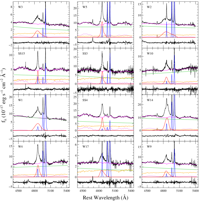
Figure 1.— Multi-component spectral decomposition for 12 objects. The observed spectra are shown along with the best-fit models. In each panel, observed spectra (black) and the continuum$+$Fe II$+$stellar best-fit model (magenta) are shown in the upper part, and the best-fit power-law continuum (green), stellar template (yellow), and Fe II template (violet) models are presented in the middle part. Three narrow lines [H$\beta$, [O III] $\lambda\lambda 4959,5007$ (blue)], broad H$\beta$ (red), and the broad and narrow He II $\lambda 4686$ components (brown; only included if blended with H$\beta$) are presented in the bottom part. The residuals (black), representing the difference between the observed spectra and the sum of all model components, are arbitrarily shifted downward for clarity.

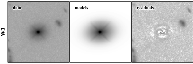
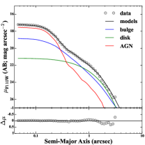
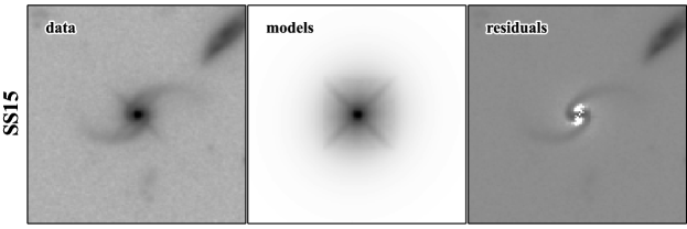
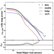
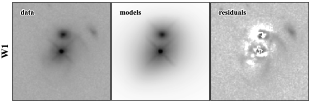
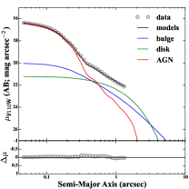
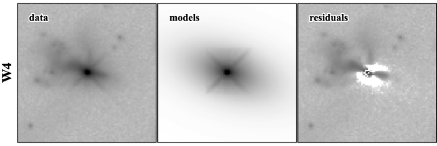
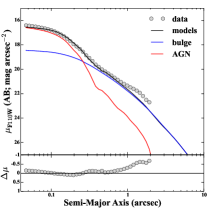
Figure 2.— HST WFC3 F110W images for 12 objects. In each row, observed data (first column), best-fit models (second column), and residuals (third column) are presented with the object name. All images are $10.8\arcsec\times 10.8\arcsec$ in size and displayed with an inverted asinh stretch. The fourth column shows the corresponding one-dimensional surface brightness profiles. In each top panel, the profiles measured from the data (open circles), the best-fit model (black solid line), and the sub-components of the model for bulge (blue solid line), disk (green solid line), AGN (red solid line) are shown. Residuals (gray circles), the difference of the profiles between the data and the best-fit model, are presented in each bottom panel. Note that the one-dimensional surface brightness profiles are shown for illustration purposes only, the actual fitting made use of the full two-dimensional images.

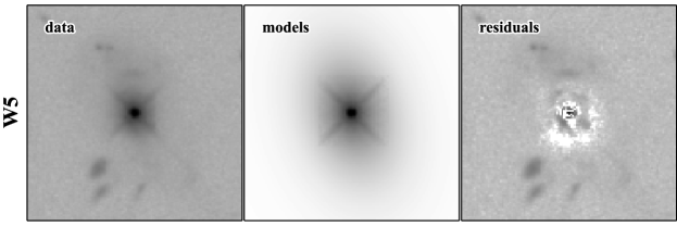
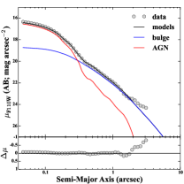
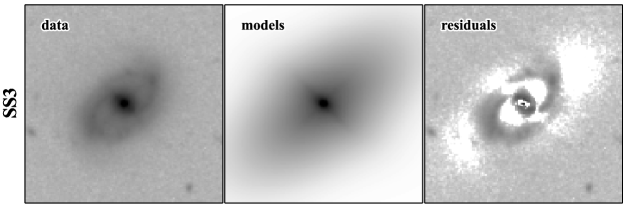
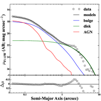
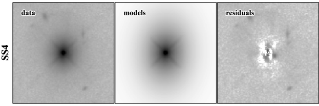
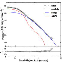
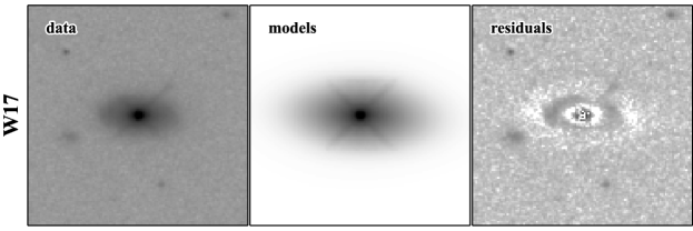
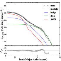
Figure 2.— Continued.

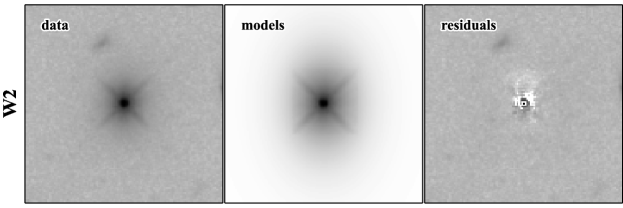
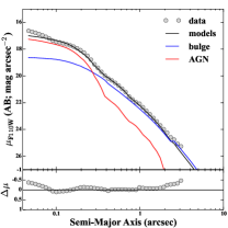
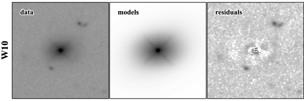
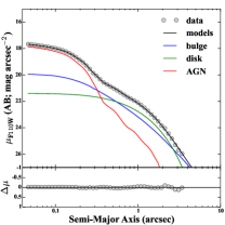
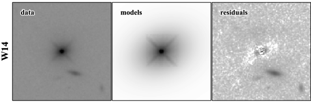
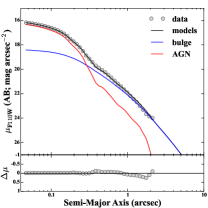
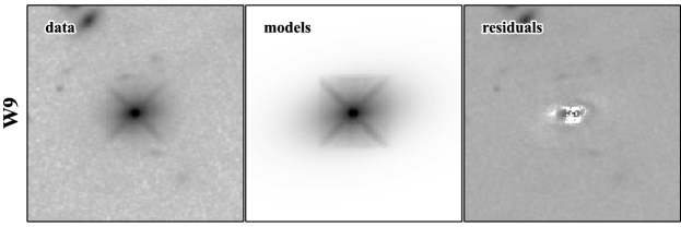
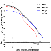
Figure 2.— Continued.

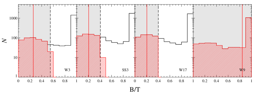
Figure 5.— Bulge-to-total (B/T) luminosity ratio distributions using informative priors from Benson et al. (2007) to estimate $L_{\rm bul}$ for those four objects with upper limits. The black histograms indicate B/T prior distributions from SDSS galaxies that have total magnitudes within $\pm 0.5$ mag to those of our active galaxy sample. The vertical black dashed line shows an upper limit value for the B/T measured from our surface photometry and the B/T likelihood function as the form of a step function is displayed as a grey shade. The posterior distribution for the B/T ratios, derived by combining the prior (black histogram) and likelihood (gray shade), is plotted as a red hashed histogram with its mean value (vertical red solid line) in each panel.

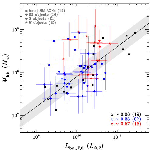
Figure 6.— $M_{\rm BH}-L_{\rm bul}$ relation. Colored symbols indicate our intermediate-$z$ sample (plus signs: SS objects; circles: S objects; stars: W objects; see Sec. 2.1 for the details of the sample). Corresponding redshifts of the samples are expressed by different colors (black: local ($\bar{z}\sim 0.08$); blue: $z=0.36$; red: $z=0.57$). The black filled squares are the local RM AGNs taken from Bennert et al. (2010) with the best-fit relation (black solid line) and its intrinsic scatter (0.21 dex; gray shaded region).

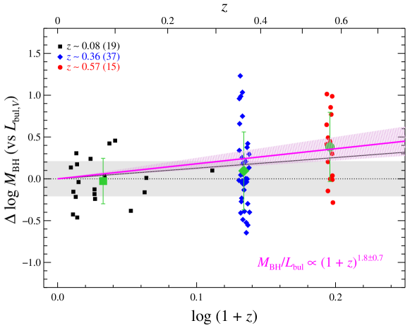
Figure 7.— Redshift evolution of the offset in $\log M_{\rm BH}$ for a given $L_{\rm bul}$ with respect to local baseline $M_{\rm BH}-L_{\rm bul}$ relation (black dotted line with gray shaded region showing the intrinsic scatter). Colored symbols indicate local RM AGNs (black squares at $\bar{z}\sim 0.08$) and our intermediate-$z$ sample at $z=0.36$ (blue diamonds) and at $z=0.57$ (red circles). The mean and root-mean-square (rms) scatter of offsets for each sample are shown as green big symbols with error bars. The black solid line represents the best-fit trend for all intermediate-$z$ objects in the functional form of $\Delta\log M_{\rm BH}=\gamma\log(1+z)$ without taking into account for selection effects. The magenta solid line with the hatched $1\sigma$ confidence range shows the result when taking into account selection effects. The corresponding best-fit value for the evolution slope is given in the lower right corner.

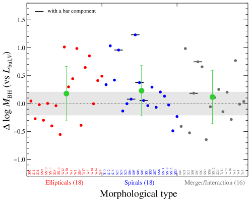
Figure 8.— The measured offset in $\log M_{\rm BH}$ for a given $L_{\rm bul}$ with respect to local baseline $M_{\rm BH}-L_{\rm bul}$ relation (black dotted line with gray shaded region for the intrinsic scatter) with simple morphological type classification based on the visual inspection of HST images. Objects containing a bar component are indicated with a black horizontal bar.

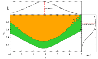
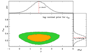
Figure 9.— Monte Carlo simulation results constraining the evolution of $\Delta\log M_{\rm BH}=\gamma\log(1+z)$ with intrinsic scatter $\sigma_{\rm int}$, by taking into account selection effects. Upper panel: Evolutionary trend assuming uniform priors; neither slope nor scatter are well constrained. Bottom panel: the same as in the upper panel, but assuming a log-normal prior for $\sigma_{\rm int}$ (Bennert et al., 2010, $\sigma_{\rm int}=0.21\pm 0.08$). The 2D posterior distributions of $\gamma$ and $\sigma_{\rm int}$ are plotted with a yellow (green) filled contour corresponding to 1$\sigma$ (2$\sigma$) confidence level. The marginalized 1D distributions for each parameter are shown in the top and right sides in each panel with the adopted best-fit values (red dashed lines) and 1$\sigma$ uncertainties.

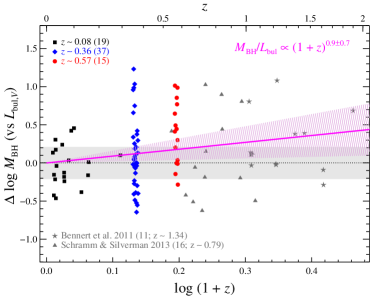
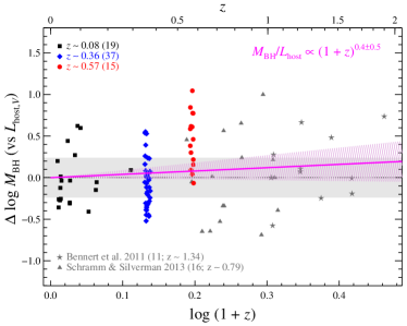
Figure 10.— Same as Figure 7, but with the additional samples from Bennert et al. (2011b) and Schramm & Silverman (2013). Left (right) panel shows the evolution of the mass offset for a given $L_{\rm bul}$ ($L_{\rm host}$) with respect to the local baseline $M_{\rm BH}-L_{\rm bul}$ ($M_{\rm BH}-L_{\rm host}$) relation. The best-fit evolution slope ($\gamma$) estimated from the Monte Carlo simulation incorporating selection effects is given at each upper right corner and over-plotted as a magenta solid line with a hatched $1\sigma$ confidence range.

Table 1Sample

Object	SDSS name	$z$	$D_{\rm L}$	$E(B-V)$
			(Mpc)	(mag)
(1)	(2)	(3)	(4)	(5)
Sample presented in Treu et al. (2007)
S09	$\rm SDSS-J005916.10+153816.0$	0.354488	1884.8	0.089
S10	$\rm SDSS-J010112.06-094500.7$	0.351342	1865.3	0.030
S12	$\rm SDSS-J021340.59+134756.0$	0.358309	1908.6	0.104
S21	$\rm SDSS-J110556.18+031243.1$	0.354551	1885.2	0.048
S16	$\rm SDSS-J111937.58+005620.3$	0.370213	1983.1	0.033
S23	$\rm SDSS-J140016.65-010822.1$	0.351314	1865.1	0.039
S24	$\rm SDSS-J140034.70+004733.3$	0.361910	1931.1	0.032
S26	$\rm SDSS-J152922.24+592854.5$	0.369242	1977.0	0.014
S27	$\rm SDSS-J153651.27+541442.6$	0.366873	1962.1	0.020
S01	$\rm SDSS-J153916.24+032322.0$	0.359351	1915.1	0.058
S02	$\rm SDSS-J161111.66+513131.1$	0.354384	1884.2	0.021
S03	$\rm SDSS-J173203.08+611751.8$	0.358429	1909.3	0.040
S04	$\rm SDSS-J210211.50-064645.0$	0.357906	1906.1	0.076
S05	$\rm SDSS-J210451.83-071209.4$	0.353505	1878.7	0.086
S06	$\rm SDSS-J212034.18-064122.2$	0.368817	1974.3	0.186
S07	$\rm SDSS-J230946.07+000048.9$	0.351999	1869.3	0.041
S08	$\rm SDSS-J235953.44-093655.6$	0.358619	1910.5	0.030
Sample presented in Bennert et al. (2010)
S11	$\rm SDSS-J010715.97-083429.4$	0.355877	1893.4	0.049
SS1	$\rm SDSS-J080427.99+522306.2$	0.356555	1897.7	0.043
SS2	$\rm SDSS-J093455.60+051409.1$	0.367083	1963.4	0.033
SS5	$\rm SDSS-J100706.26+084228.4$	0.373450	2003.5	0.029
S31	$\rm SDSS-J101527.26+625911.5$	0.350568	1860.5	0.006
SS6	$\rm SDSS-J102103.58+304755.9$	0.358781	1911.5	0.025
SS7	$\rm SDSS-J104331.50-010732.8$	0.361284	1927.1	0.046
SS8	$\rm SDSS-J104610.60+035031.2$	0.365515	1953.6	0.039
SS9	$\rm SDSS-J125838.71+455515.5$	0.370188	1982.9	0.012
SS10	$\rm SDSS-J133414.84+114221.5$	0.365808	1955.5	0.023
SS11	$\rm SDSS-J135226.90+392426.8$	0.373111	2001.3	0.016
SS12	$\rm SDSS-J150116.82+533102.1$	0.362919	1937.4	0.013
SS13	$\rm SDSS-J150541.79+493520.0$	0.374316	2008.9	0.013
S28	$\rm SDSS-J161156.29+451610.9$	0.367841	1968.2	0.011
SS14	$\rm SDSS-J211531.68-072627.5$	0.370558	1985.3	0.117
S29	$\rm SDSS-J215841.92-011500.3$	0.357366	1902.7	0.083
SS18	$\rm SDSS-J234050.52+010635.5$	0.358543	1910.0	0.029
W11	$\rm SDSS-J015516.18-094556.0$	0.565000	3282.3	0.019
W22	$\rm SDSS-J034229.70-052319.4$	0.565167	3283.5	0.042
W12	$\rm SDSS-J143955.10+355305.3$	0.562309	3263.4	0.010
W20	$\rm SDSS-J150014.81+322940.4$	0.576130	3360.7	0.014
W16	$\rm SDSS-J152654.93-003243.3$	0.578015	3374.0	0.106
W8	$\rm SDSS-J163252.42+263749.1$	0.571209	3326.0	0.043
Sample presented here
W3	$\rm SDSS-J002005.69-005016.3$	0.576049	3360.1	0.024
SS15	$\rm SDSS-J014412.77-000610.5$	0.359329	1914.9	0.024
W1	$\rm SDSS-J083654.98+075712.4$	0.573637	3343.1	0.026
W4	$\rm SDSS-J093210.96+433813.1$	0.576601	3364.0	0.018
W5	$\rm SDSS-J094852.73+363120.5$	0.576728	3364.9	0.012
SS3	$\rm SDSS-J095553.14+633742.8$	0.356623	1898.1	0.028
SS4	$\rm SDSS-J095850.15+400342.3$	0.362909	1937.3	0.011
W17	$\rm SDSS-J100728.38+392651.8$	0.561690	3259.0	0.012
W2	$\rm SDSS-J110641.86+614146.5$	0.572026	3331.7	0.008
W10	$\rm SDSS-J111415.83-005920.4$	0.571076	3325.0	0.035
W14	$\rm SDSS-J125631.89-023130.6$	0.561702	3259.1	0.019
W9	$\rm SDSS-J155227.81+562236.4$	0.565356	3284.8	0.010

Note. — Column 1: Object ID. Column 2: SDSS name. Column 3: Redshifts as listed in NED from improved redshifts by Hewett & Wild (2010). Column 4: Luminosity distance. Column 5: $E(B-V)$ as listed in NED from the Schlafly & Finkbeiner (2011) recalibration of the Schlegel et al. (1998) infrared-based dust map.

Table 2Results from Keck spectroscopic analysis

Object	S/N	FWHMHβ	$\sigma_{\rm H\beta}$	$\lambda L_{5100}^{\rm spec}$	$\log M_{\rm BH}^{\rm spec}$
	(pix-1)	(km s-1)	(km s-1)	($10^{44}$erg s-1)	($M_{\odot}$)
(1)	(2)	(3)	(4)	(5)	(6)
S09	39	2655	1748	1.76	8.15
S10	96	4850	2597	2.77	8.59
S12	40	8800	4256	1.82	8.93
S21	75	8296	3897	5.33	9.09
S16	6	3749	1867	0.69	8.00
S23	108	9629	4251	1.78	8.92
S24	100	7061	2635	1.49	8.47
S26	50	5386	1914	0.83	8.06
S27	42	2508	1409	1.26	7.89
S01	69	4662	2194	1.37	8.29
S02	44	4841	2274	1.25	8.30
S03	88	3018	1716	2.11	8.17
S04	46	2821	1749	1.19	8.06
S05	119	4908	3333	2.23	8.76
S06	31	4527	1413	1.10	7.86
S07	108	4635	2547	1.81	8.48
S08	54	2909	1217	1.59	7.81
S11	114	2595	1354	1.57	7.90
SS1	26	2620	1501	1.04	7.90
SS2	32	2815	1316	0.83	7.73
SS5	46	2790	1612	1.40	8.03
S31	79	4012	2117	0.93	8.17
SS6	48	1947	1031	0.69	7.48
SS7	54	2959	1371	0.98	7.81
SS8	82	2733	1532	1.54	8.00
SS9	70	2787	1569	1.25	7.98
SS10	84	2232	1431	4.09	8.16
SS11	49	3505	1466	2.07	8.03
SS12	116	2101	1371	4.34	8.14
SS13	108	2169	1143	1.49	7.74
S28	73	4600	2532	0.97	8.33
SS14	51	2143	1212	0.65	7.60
S29	54	3533	1847	1.20	8.11
SS18	63	1631	1029	1.90	7.71
W11	18	3812	2026	0.78	8.09
W22	81	5835	2654	4.65	8.73
W12	63	7698	3859	3.62	9.00
W20	26	10861	3806	1.33	8.76
W16	37	2392	1564	1.05	7.94
W8	57	7340	2977	4.17	8.81
W3	59	7461	3508	1.47	8.71
SS15	46	1604	1000	0.64	7.43
W1	80	7378	3152	4.71	8.88
W4	51	3490	1728	3.68	8.30
W5	72	2722	1738	4.94	8.38
SS3	13	1953	1252	0.74	7.66
SS4	64	2213	1378	1.35	7.88
W17	24	5556	2483	0.86	8.29
W2	66	12647	4811	3.03	9.15
W10	31	3636	1477	2.92	8.12
W14	76	5001	2616	5.56	8.76
W9	62	5273	2747	2.64	8.63

Note. — Column 1: Object ID. Column 2: S/N averaged at rest wavelength range of 5080–5120 Å. Column 3: FWHM of H$\beta$ broad emission line. Column 4: Line dispersion of H$\beta$ broad emission line. Column 5: Continuum luminosities at 5100 Å as measured from spectra. Column 6: BH mass derived from Eq (1) using $\sigma_{\rm H\beta}$ and $\lambda L_{5100}^{\rm spec}$ measurements. Note that all spectroscopic properties and BH mass estimates are updated from Woo et al. (2006, 2008).

Table 3Results from HST image analysis

Object	Instrument/Filter	Ncomp.	Total	PSF	Host	Bulge	$r_{\rm eff,bul}$	$r_{\rm eff,bul}$	$f_{\rm AGN}$	$\lambda L_{5100}^{\rm image}$	$\log L_{{\rm host},V}$	$\log L_{{\rm bul},V}$
			(mag)	(mag)	(mag)	(mag)	($\arcsec$)	(kpc)		($10^{44}$erg s-1)	($L_{\odot,V}$)	($L_{\odot,V}$)
(1)	(2)	(3)	(4)	(5)	(6)	(7)	(8)	(9)	(10)	(11)	(12)	(13)
S09	ACS/F775W	3	18.10	19.67	18.39	18.46	2.60	12.97	0.23	0.86	10.95	10.93
S10	ACS/F775W	3	17.96	19.13	18.41	19.49	0.11	0.52	0.34	1.38	10.93	10.50
S12	ACS/F775W	3	18.17	19.58	18.52	20.79	0.17	0.85	0.27	0.96	10.92	10.01
S21	ACS/F775W	3	17.32	18.51	17.77	19.07	0.10	0.50	0.34	2.52	11.20	10.68
S16	ACS/F775W	3	19.11	19.91	19.82	21.42	0.41	2.12	0.48	0.76	10.43	9.79
S23	ACS/F775W	4	18.01	19.33	18.39	20.33	0.24	1.18	0.30	1.15	10.94	10.17
S24	ACS/F775W	3	18.10	20.41	18.24	18.72	1.83	9.24	0.12	0.46	11.04	10.85
S26	ACS/F775W	3	18.84	20.10	19.24	19.97	0.24	1.25	0.31	0.64	10.66	10.37
S27	ACS/F775W	3	18.11	19.52	18.45	18.62	4.71	23.98	0.27	1.07	10.97	10.90
S01	ACS/F775W	4	18.53	19.89	18.89	20.05	0.97	4.87	0.28	0.72	10.77	10.31
S02	ACS/F775W	3	19.03	20.61	19.32	19.96	0.45	2.25	0.23	0.36	10.58	10.33
S03	ACS/F775W	4	17.89	18.74	18.56	21.36	0.10	0.51	0.46	2.08	10.90	9.78
S04	ACS/F775W	4	18.07	19.11	18.60	19.79	0.41	2.03	0.38	1.47	10.88	10.41
S05	ACS/F775W	4	17.97	18.77	18.68	21.06	0.10	0.50	0.48	1.96	10.84	9.88
S06	ACS/F775W	4	18.51	20.17	18.78	21.69	0.10	0.53	0.22	0.59	10.85	9.68
S07	ACS/F775W	3	17.78	18.62	18.44	20.32	0.24	1.20	0.46	2.22	10.92	10.18
S08	ACS/F775W	4	18.31	19.35	18.83	21.00	0.17	0.88	0.38	1.18	10.79	9.92
S11	NICMOS/F110W	3	17.86	19.54	18.11	19.10	0.10	0.51	0.21	0.83	10.80	10.40
SS1	NICMOS/F110W	3	17.88	20.10	18.03	19.37	0.10	0.48	0.13	0.50	10.84	10.30
SS2	NICMOS/F110W	2	18.37	20.46	18.55	18.55	0.38	1.96	0.15	0.38	10.66	10.66
SS5	NICMOS/F110W	3	18.31	19.33	18.85	19.65	0.10	0.50	0.39	1.12	10.56	10.24
S31	NICMOS/F110W	3	17.56	19.27	17.81	18.41	1.25	6.17	0.21	1.02	10.90	10.66
SS6	NICMOS/F110W	3	18.84	20.19	19.20	20.38	0.10	0.48	0.29	0.46	10.37	9.90
SS7	NICMOS/F110W	3	18.30	20.07	18.54	19.41	0.10	0.49	0.20	0.53	10.64	10.30
SS8	NICMOS/F110W	3	17.89	19.67	18.12	19.95	0.10	0.49	0.19	0.78	10.82	10.09
SS9	NICMOS/F110W	2	18.02	19.33	18.41	18.41	0.31	1.57	0.30	1.09	10.72	10.72
SS10	NICMOS/F110W	3	17.55	18.19	18.42	18.92	0.10	0.51	0.55	3.05	10.71	10.51
SS11	NICMOS/F110W	3	18.11	19.65	18.41	19.75	0.10	0.49	0.24	0.83	10.73	10.19
SS12	NICMOS/F110W	2	17.37	17.73	18.75	18.75	0.10	0.48	0.72	4.61	10.56	10.56
SS13	NICMOS/F110W	2	18.38	19.29	19.00	19.00	0.23	1.16	0.43	1.17	10.50	10.50
S28	NICMOS/F110W	3	18.05	20.48	18.17	18.70	0.32	1.64	0.11	0.37	10.81	10.60
SS14	NICMOS/F110W	2	19.00	20.65	19.27	19.27	0.29	1.49	0.22	0.33	10.38	10.38
S29	NICMOS/F110W	3	18.36	19.92	18.66	19.50	0.10	0.48	0.24	0.59	10.59	10.25
SS18	NICMOS/F110W	3	18.39	19.58	18.83	20.13	0.10	0.48	0.33	0.81	10.52	10.00
W11	NICMOS/F110W	2	19.62	21.41	19.85	19.85	0.28	1.83	0.19	0.41	10.63	10.63
W22	NICMOS/F110W	2	17.99	19.05	18.50	18.50	1.15	7.46	0.38	3.65	11.17	11.17
W12	NICMOS/F110W	3	18.51	19.31	19.21	19.59	0.10	0.62	0.48	2.84	10.88	10.73
W20	NICMOS/F110W	2	18.98	20.99	19.17	19.17	0.49	3.20	0.16	0.64	10.93	10.93
W16	NICMOS/F110W	2	19.38	20.82	19.72	19.72	0.17	1.12	0.27	0.75	10.71	10.71
W8	NICMOS/F110W	2	18.46	19.26	19.17	19.17	0.23	1.49	0.48	3.07	10.91	10.91
W3	WFC3/F110W	3	18.84	19.80	19.43	20.08	0.23	1.48	0.41	1.85	10.78	10.52
SS15	WFC3/F110W	2	18.81	19.79	19.38	19.38	0.26	1.32	0.41	0.65	10.26	10.26
W1	WFC3/F110W	3	18.33	18.96	19.22	19.84	1.17	7.67	0.56	3.97	10.85	10.61
W4	WFC3/F110W	2	18.38	19.19	19.09	19.09	0.48	3.15	0.48	3.26	10.91	10.91
W5	WFC3/F110W	2	18.44	19.17	19.22	19.22	0.60	3.91	0.51	3.32	10.86	10.86
SS3	WFC3/F110W	3	18.16	20.37	18.31	19.28	0.23	1.13	0.13	0.38	10.68	10.29
SS4	WFC3/F110W	2	17.88	19.17	18.28	18.28	0.50	2.53	0.31	1.18	10.71	10.71
W17	WFC3/F110W	3	19.15	20.46	19.53	20.52	0.23	1.46	0.30	0.95	10.70	10.31
W2	WFC3/F110W	2	18.70	19.61	19.31	19.31	0.47	3.04	0.43	2.17	10.81	10.81
W10	WFC3/F110W	3	19.12	20.15	19.65	20.31	0.68	4.42	0.39	1.31	10.67	10.41
W14	WFC3/F110W	2	18.27	18.93	19.12	19.12	0.49	3.19	0.54	3.89	10.87	10.87
W9	WFC3/F110W	2	18.36	19.06	19.16	19.16	0.23	1.46	0.52	3.50	10.86	10.86

Note. — Column 1: Object ID. Column 2: HST instrument and filter. Column 3: Number of model components fitted (2=PSF+Bulge; 3=PSF+Bulge+Disk; 4=PSF+Bulge+Disk+Bar). Column 4: Total extinction-corrected AB magnitude (Total=PSF+Bulge+(Disk)+(Bar)). Column 5: AGN extinction-corrected AB magnitude (from PSF). Column 6: Host-galaxy extinction-corrected AB magnitude (Host=Bulge+(Disk)+(Bar)). Column 7: Bulge extinction-corrected AB magnitude. Column 8: Bulge effective radius in arcsec. Column 9: Bulge effective radius in kpc. Column 10: AGN-to-total light fraction. Column 11: AGN continuum luminosities at rest-frame 5100 Å in $10^{44}$ erg s^-1 measured from images. Column 12: Host-galaxy luminosity in rest-frame $V$ (solar units), not corrected for evolution. Column 13: Bulge luminosity in rest-frame $V$ (solar units), not corrected for evolution.

Table 4Resulting $M_{\rm BH}$ and $L_{\rm bul}$

Object	$\log M_{\rm BH}$	$\log L_{{\rm bul},V}$	$\log L_{{\rm bul},V,0}$
	($M_{\odot}$)	($L_{\odot,V}$)	($L_{\odot,V}$)
(1)	(2)	(3)	(4)
S09	7.99	10.93	10.71
S10	8.44	10.50	10.29
S12	8.78	10.01	9.79
S21	8.93	10.28	10.06
S16	8.02	9.79	9.56
S23	8.82	10.17	9.95
S24	8.20	10.85	10.62
S26	8.00	10.37	10.14
S27	7.85	10.90	10.68
S01	8.15	10.31	10.09
S02	8.02	10.33	10.11
S03	8.17	9.54	9.32
S04	8.11	10.41	10.18
S05	8.73	9.65	9.43
S06	7.72	9.43	9.20
S07	8.53	10.18	9.96
S08	7.74	9.92	9.70
S11	7.76	10.40	10.18
SS1	7.73	10.03	9.81
SS2	7.56	10.66	10.43
SS5	7.98	9.92	9.69
S31	8.19	10.66	10.45
SS6	7.39	9.57	9.35
SS7	7.67	9.98	9.76
SS8	7.85	9.86	9.63
SS9	7.95	10.72	10.49
SS10	8.10	10.51	10.28
SS11	7.83	9.94	9.71
SS12	8.15	10.44	10.21
SS13	7.69	10.50	10.27
S28	8.12	10.60	10.37
SS14	7.45	10.38	10.15
S29	7.95	9.93	9.71
SS18	7.51	9.71	9.48
W11	7.95	10.63	10.28
W22	8.68	11.17	10.82
W12	8.94	10.39	10.04
W20	8.60	10.93	10.57
W16	7.86	10.71	10.35
W8	8.74	10.91	10.56
W3	8.76	10.18	9.83
SS15	7.44	10.26	10.04
W1	8.84	10.61	10.25
W4	8.28	10.91	10.55
W5	8.29	10.86	10.50
SS3	7.51	10.00	9.78
SS4	7.85	10.71	10.49
W17	8.31	10.02	9.67
W2	9.07	10.81	10.46
W10	7.94	10.41	10.05
W14	8.68	10.87	10.52
W9	8.70	10.79	10.44

Note. — Column 1: Object ID. Column 2: BH mass derived from Eq. (1) using $\sigma_{\rm H\beta}$ and $\lambda L_{5100}^{\rm image}$ (in solar units). Column 3: Bulge luminosity in rest-frame $V$ (in solar units). For 18 objects with upper limits, the bulge luminosity was derived using informative priors (see Section 3.2 for details). Column 4: Final bulge luminosity corrected for evolution by aging of the stellar population.

Appendix A Updated Measurements of Previous Sample

We performed a consistent spectral and image analysis for 40 objects presented by Treu et al. (2007) and Bennert et al. (2010), using the same methods described in the main text to minimize measurement systematics (see Figure 11 and 14).

We compare the previous and new measurements for BH masses and bulge luminosities in Figure 22. On average we obtained consistent measurements with previous results (i.e., close to zero offsets). However, there is a considerable scatter ($\sim 0.18$ dex for $M_{\rm BH}$ and $\sim 0.22$ dex for $L_{\rm bul}$), indicating the necessity of a homogeneous and careful analysis. We consider the results presented here more robust, given several improvements in the analysis. For one, the multi-component spectral decomposition applied here takes into account host-galaxy starlight contribution as well as iron emission blends for a better isolation of the broad H$\beta$ emission line, resulting in a more accurate measurement of BH mass. The difference between the previous and new line width ($\sigma_{\rm line}$) is $\sim 0.08$ dex scatter. Second, the current multi-component image decomposition has advantages over the previous approach. It not only achieves a better optimization by probing the true global minimum over parameter spaces, but the PSF model consisting of a linear combination of several field stars minimizes any PSF mismatch and arguably provides more accurate structural decomposition results. Moreover, in contrast to the previous approach, our model allows off-centered AGN and galaxy components for a given object.

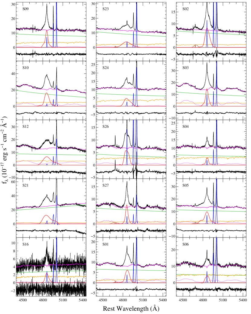
Figure 11.— Same as Figure 1, but for the previous sample of 40 objects.

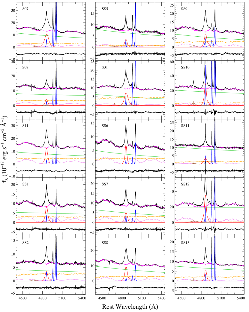
Figure A1.— Continued.

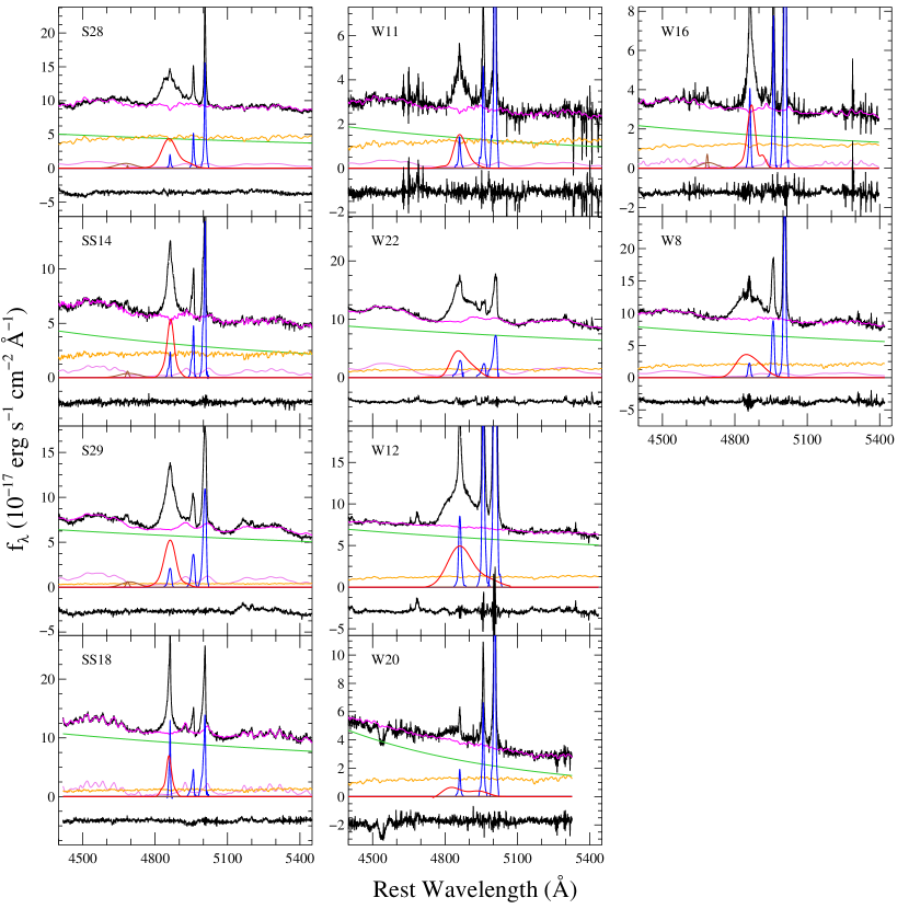
Figure A1.— Continued.

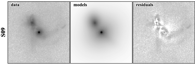
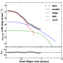
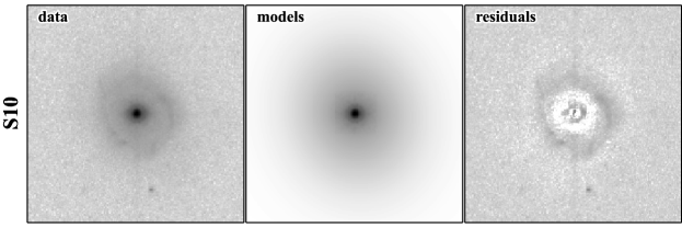
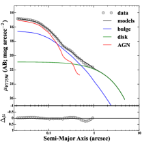
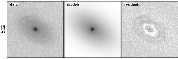
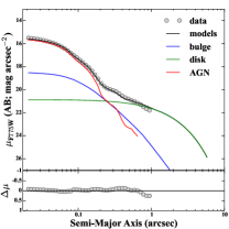
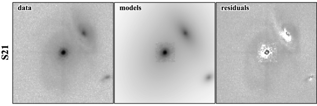
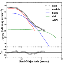
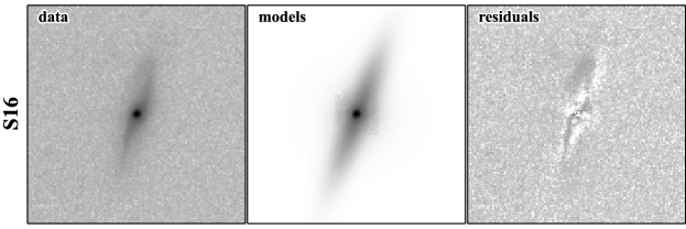
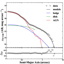
Figure 14.— Same as Figure 2, but for the previous sample of 40 objects with displayed image sizes of $8\arcsec\times 8\arcsec$ (HST ACS images; first 17 objects) and $7.6\arcsec\times 7.6\arcsec$ (HST NICMOS images; next 23 objects).

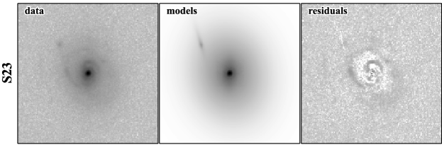
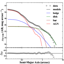
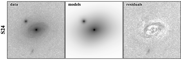
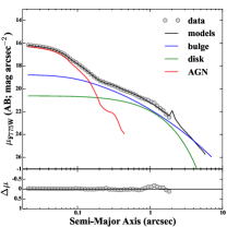
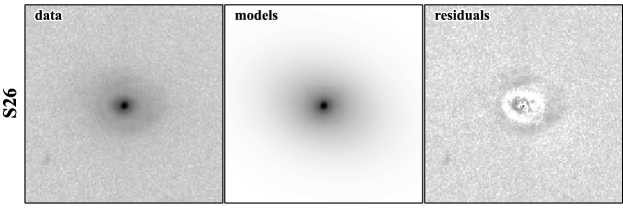
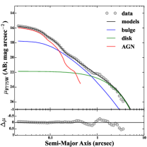
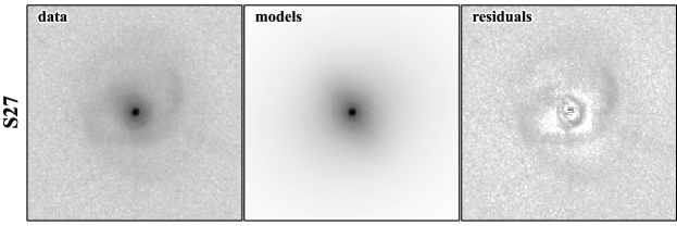
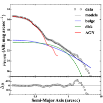
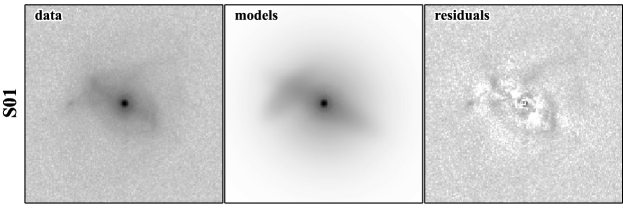
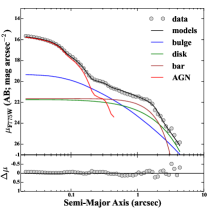
Figure A2.— Continued.

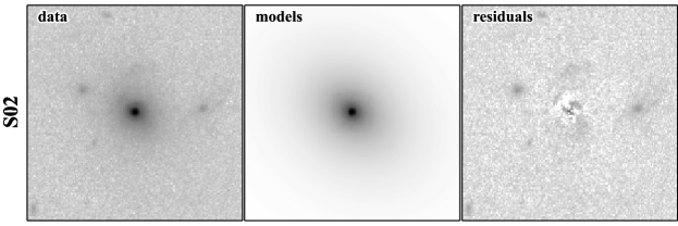
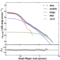
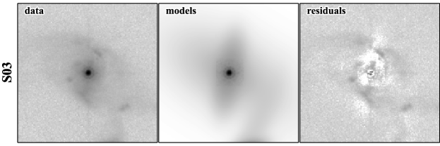
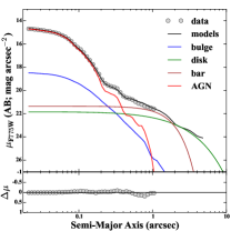
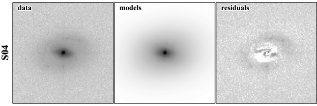
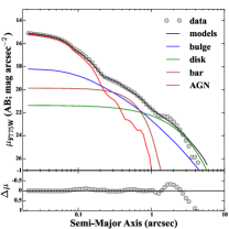
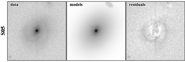
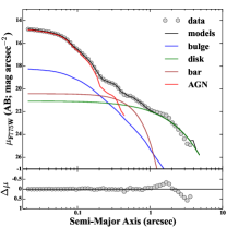
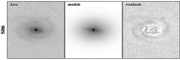
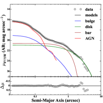
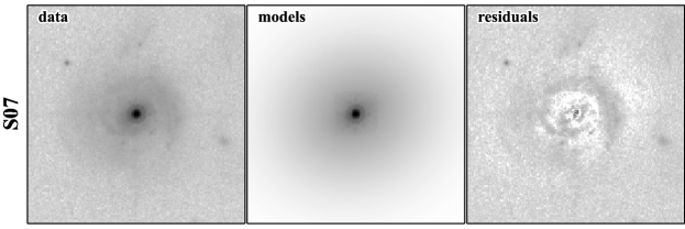
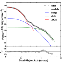
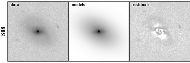
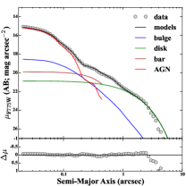
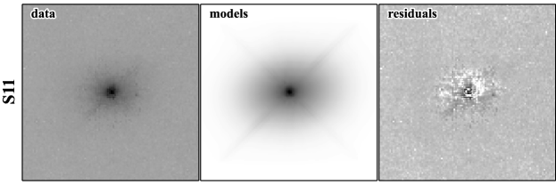
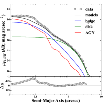
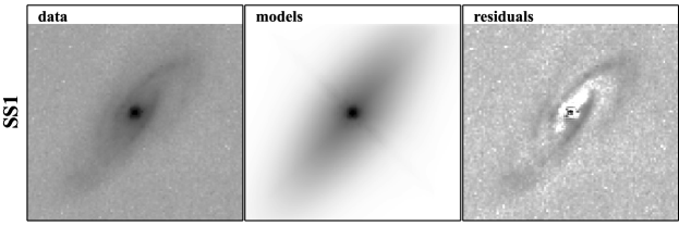
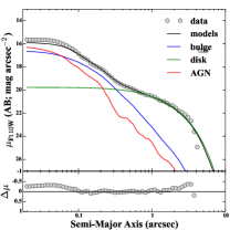
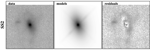
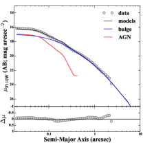
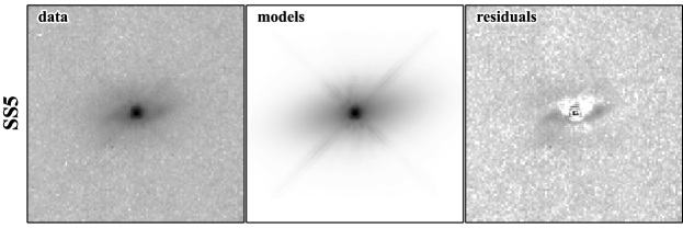
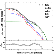
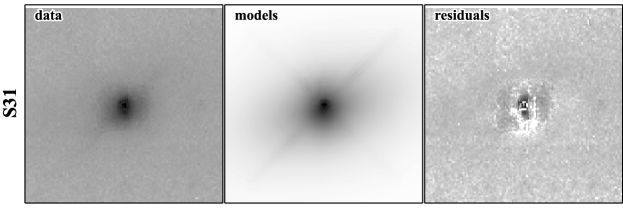
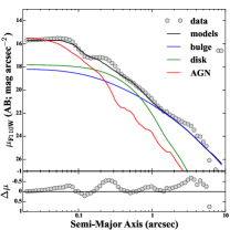
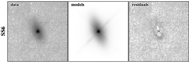
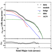
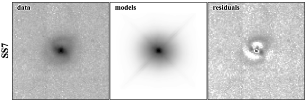
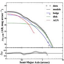
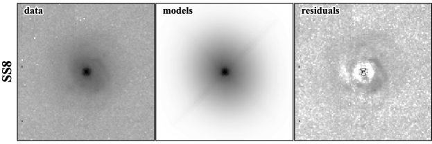
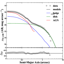
Figure A2.— Continued.

Figure A2.— Continued.

Figure A2.— Continued.

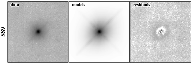
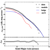
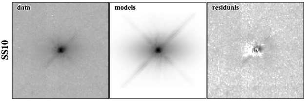
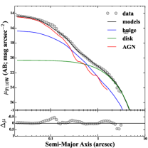
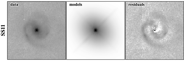
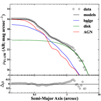
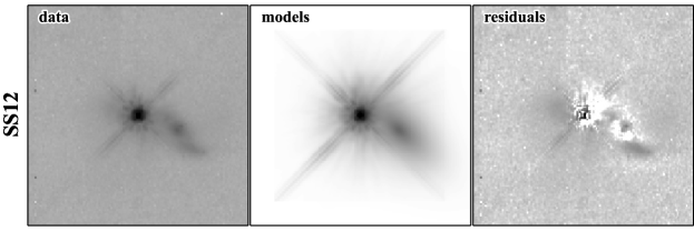
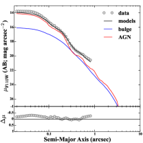
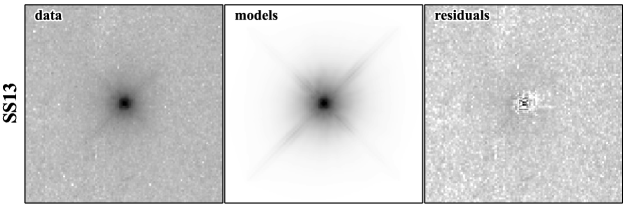
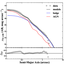
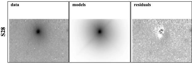
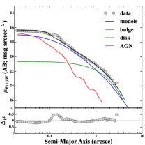
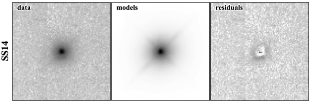
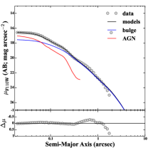
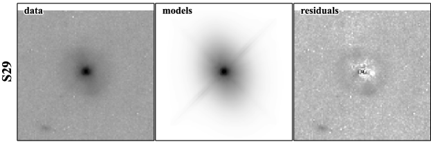
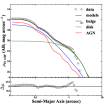
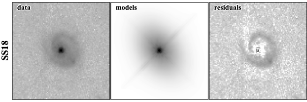
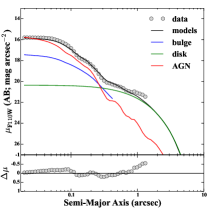
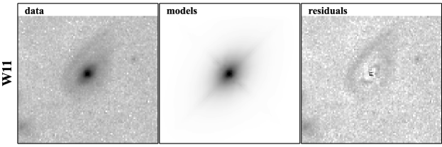
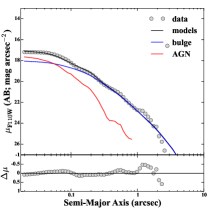
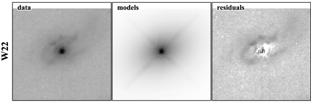
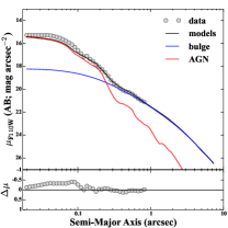
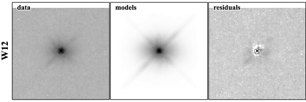
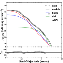
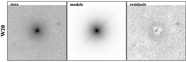
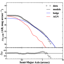
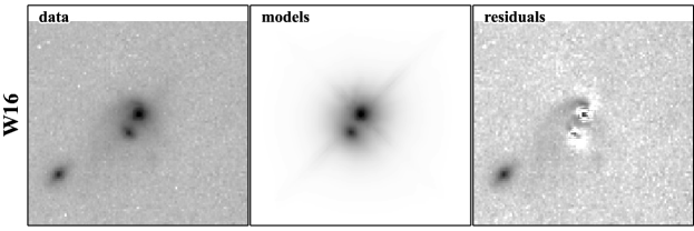
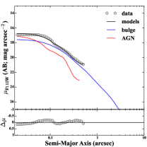
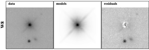
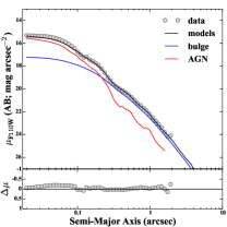
Figure A2.— Continued.

Figure A2.— Continued.

Figure A2.— Continued.

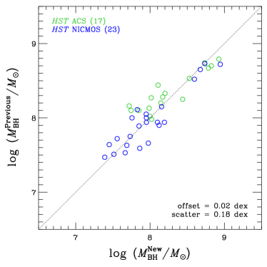
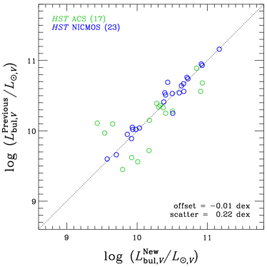
Figure 22.— Difference of BH mass estimates (left) and bulge luminosity estimates (right) between previous results (Bennert et al., 2010) and new results presented here.

Appendix B Comparison between $\lambda L_{5100}^{\rm spec}$ and $\lambda L_{5100}^{\rm image}$

Figure 23 compares AGN continuum luminosities, $\lambda L_{5100}$, measured from spectra and images. There are considerable offset and scatter between them due to several possible reasons. In addition to AGN intrinsic variability and seeing effects, the adopted single power-law SED when converting PSF magnitudes into luminosities at $5100$ Å (Sec. 3.2) will contribute some amount of the scatter. The AGN continuum luminosities measured from spectra are on average larger than those from images by $\sim 0.17$ dex. This is probably because the AGN luminosity measured from spectra could be overestimated from the different contribution of host galaxy starlights, which is stemming from aperture size difference between Keck slit and Sloan fiber spectra when performing flux (re-)calibration (Sec. 2.2). Although the scatter between AGN luminosities estimated from spectra and images is reduced significantly (by $\sim 0.2$ dex) after the renormalization, the overall flux scale could be increased against the genuine value due to the smaller contribution of host galaxy in Keck spectra than that of Sloan spectra if the amount of AGN variability is marginal. There is another possibility of the overestimation when performing spectral decomposition in that the AGN power-law model could be contaminated with the contribution from young stellar population (if any) since it is not possible to decompose it unambiguously with this limited wavelength range of the spectra.

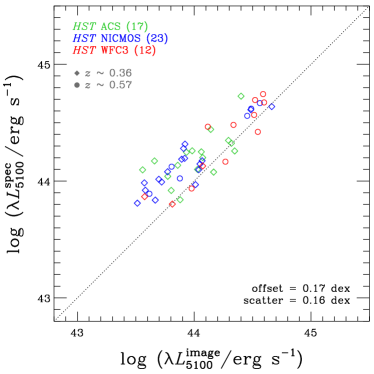
Figure 23.— Difference of AGN continuum luminosity estimates from Keck spectra and HST images for all 52 objects.

References

- Alexander et al. (2008) Alexander, D. M., Brandt, W. N., Smail, I., et al. 2008, AJ, 135, 1968
- Anglés-Alcázar et al. (2013a) Anglés-Alcázar, D., Özel, F., & Davé, R. 2013a, ApJ, 770, 5
- Anglés-Alcázar et al. (2013b) Anglés-Alcázar, D., Özel, F., Davé, R., et al. 2013b, ApJ submitted (arXiv:1309.5963)
- Beifiori et al. (2011) Beifiori, A., Maraston, C., Thomas, D., & Johansson, J. 2011, A&A, 531, A109
- Beifiori et al. (2012) Beifiori, A., Courteau, S., Corsini, E. M., & Zhu, Y. 2012, MNRAS, 419, 2497
- Bennert et al. (2010) Bennert, V. N., Treu, T., Woo, J.-H., et al. 2010, ApJ, 708, 1507
- Bennert et al. (2011a) Bennert, V. N., Auger, M. W., Treu, T., Woo, J.-H., & Malkan, M. A. 2011a, ApJ, 726, 59
- Bennert et al. (2011b) Bennert, V. N., Auger, M. W., Treu, T., Woo, J.-H., & Malkan, M. A. 2011b, ApJ, 742, 107
- Benson et al. (2007) Benson, A. J., Džanović, D., Frenk, C. S., & Sharples, R. 2007, MNRAS, 379, 841
- Bentz et al. (2006) Bentz, M. C., Peterson, B. M., Pogge, R. W., Vestergaard, M., & Onken, C. A. 2006, ApJ, 644, 133
- Bentz et al. (2009a) Bentz, M. C., Peterson, B. M., Netzer, H., Pogge, R. W., & Vestergaard, M. 2009a, ApJ, 697, 160
- Bentz et al. (2009b) Bentz, M. C., Peterson, B. M., Pogge, R. W., & Vestergaard, M. 2009b, ApJ, 694, L166
- Bentz et al. (2013) Bentz, M. C., Denney, K. D., Grier, C. J., et al. 2013, ApJ, 767, 149
- Bongiorno et al. (2014) Bongiorno, A., Maiolino, R., Brusa, M., et al. 2014, MNRAS in press (arXiv:1406.6094)
- Boroson & Green (1992) Boroson, T. A., & Green, R. F. 1992, ApJS, 80, 109
- Brewer et al. (2011) Brewer, B. J., Treu, T., Pancoast, A., et al. 2011, ApJ, 733, L33
- Bruzual & Charlot (1993) Bruzual A., G., & Charlot, S. 1993, ApJ, 405, 538
- Bruzual & Charlot (2003) Bruzual, G., & Charlot, S. 2003, MNRAS, 344, 1000
- Busch et al. (2014) Busch, G., Zuther, J., Valencia-S., M., et al. 2014, A&A, 561, A140
- Canalizo et al. (2012) Canalizo, G., Wold, M., Hiner, K. D., et al. 2012, ApJ, 760, 38
- Cao (2010) Cao, X. 2010, ApJ, 725, 388
- Cisternas et al. (2011) Cisternas, M., Jahnke, K., Bongiorno, A., et al. 2011, ApJ, 741, L11
- Coleman et al. (1980) Coleman, G. D., Wu, C.-C., & Weedman, D. W. 1980, ApJS, 43, 393
- Croton (2006) Croton, D. J. 2006, MNRAS, 369, 1808
- Croton et al. (2006) Croton, D. J., Springel, V., White, S. D. M., et al. 2006, MNRAS, 365, 11
- Croton (2009) Croton, D. J. 2009, MNRAS, 394, 1109
- Davis & Laor (2011) Davis, S. W., & Laor, A. 2011, ApJ, 728, 98
- Decarli et al. (2010) Decarli, R., Falomo, R., Treves, A., et al. 2010, MNRAS, 402, 2453
- de Vaucouleurs (1948) de Vaucouleurs, G. 1948, Annales d’Astrophysique, 11, 247
- Di Matteo et al. (2005) Di Matteo, T., Springel, V., & Hernquist, L. 2005, Nature, 433, 604
- Dubois et al. (2013) Dubois, Y., Gavazzi, R., Peirani, S., & Silk, J. 2013, MNRAS, 433, 3297
- Driver et al. (2007) Driver, S. P., Allen, P. D., Liske, J., & Graham, A. W. 2007, ApJ, 657, L85
- Ferrarese & Ford (2005) Ferrarese, L., & Ford, H. 2005, Space Sci. Rev., 116, 523
- Ferrarese & Merritt (2000) Ferrarese, L., & Merritt, D. 2000, ApJ, 539, L9
- Fernández Lorenzo et al. (2011) Fernández Lorenzo, M., Cepa, J., Bongiovanni, A., et al. 2011, A&A, 526, A72
- Fitzpatrick (1999) Fitzpatrick, E. L. 1999, PASP, 111, 63
- Furlanetto & Lidz (2011) Furlanetto, S. R., & Lidz, A. 2011, ApJ, 735, 117
- Gebhardt et al. (2000) Gebhardt, K., Bender, R., Bower, G., et al. 2000, ApJ, 539, L13
- Gilli et al. (2009) Gilli, R., Zamorani, G., Miyaji, T., et al. 2009, A&A, 494, 33
- Graham et al. (2011) Graham, A. W., Onken, C. A., Athanassoula, E., & Combes, F. 2011, MNRAS, 412, 2211
- Graham & Scott (2013) Graham, A. W., & Scott, N. 2013, ApJ, 764, 151
- Grier et al. (2013) Grier, C. J., Martini, P., Watson, L. C., et al. 2013, ApJ, 773, 90
- Gültekin et al. (2009) Gültekin, K., Richstone, D. O., Gebhardt, K., et al. 2009, ApJ, 698, 198
- Harris et al. (2012) Harris, C. E., Bennert, V. N., Auger, M. W., et al. 2012, ApJS, 201, 29
- Häring & Rix (2004) Häring, N., & Rix, H.-W. 2004, ApJ, 604, L89
- Hiner et al. (2012) Hiner, K. D., Canalizo, G., Wold, M., Brotherton, M. S., & Cales, S. L. 2012, ApJ, 756, 162
- Hirschmann et al. (2010) Hirschmann, M., Khochfar, S., Burkert, A., et al. 2010, MNRAS, 407, 1016
- Hewett & Wild (2010) Hewett, P. C., & Wild, V. 2010, MNRAS, 405, 2302
- Hopkins et al. (2005) Hopkins, P. F., Hernquist, L., Martini, P., et al. 2005, ApJ, 625, L71
- Hopkins & Hernquist (2009) Hopkins, P. F., & Hernquist, L. 2009, ApJ, 698, 1550
- Hopkins et al. (2009) Hopkins, P. F., Murray, N., & Thompson, T. A. 2009, MNRAS, 398, 303
- Jahnke et al. (2009) Jahnke, K., Bongiorno, A., Brusa, M., et al. 2009, ApJ, 706, L215
- Jahnke & Macciò (2011) Jahnke, K., & Macciò, A. V. 2011, ApJ, 734, 92
- Kauffmann & Haehnelt (2000) Kauffmann, G., & Haehnelt, M. 2000, MNRAS, 311, 576
- Kelly et al. (2010) Kelly, B. C., Vestergaard, M., Fan, X., et al. 2010, ApJ, 719, 1315
- Kim et al. (2008a) Kim, M., Ho, L. C., Peng, C. Y., et al. 2008a, ApJ, 687, 767
- Kim et al. (2008b) Kim, M., Ho, L. C., Peng, C. Y., Barth, A. J., & Im, M. 2008b, ApJS, 179, 283
- Kormendy & Ho (2013) Kormendy, J., & Ho, L. C. 2013, ARA&A, 51, 511
- Lamastra et al. (2010) Lamastra, A., Menci, N., Maiolino, R., Fiore, F., & Merloni, A. 2010, MNRAS, 405, 29
- Läsker et al. (2014) Läsker, R., Ferrarese, L., van de Ven, G., & Shankar, F. 2014, ApJ, 780, 70
- Lauer et al. (2007) Lauer, T. R., Tremaine, S., Richstone, D., & Faber, S. M. 2007, ApJ, 670, 249
- Lawson & Hanson (1987) Lawson C., Hanson R.J., 1987, Solving Least Squares Problems, SIAM
- Li et al. (2012) Li, Y.-R., Wang, J.-M., & Ho, L. C. 2012, ApJ, 749, 187
- Li et al. (2013) Li, Y.-R., Wang, J.-M., Ho, L. C., Du, P., & Bai, J.-M. 2013, ApJ, 779, 110
- Magorrian et al. (1998) Magorrian, J., Tremaine, S., Richstone, D., et al. 1998, AJ, 115, 2285
- Marconi & Hunt (2003) Marconi, A., & Hunt, L. K. 2003, ApJ, 589, L21
- Marconi et al. (2004) Marconi, A., Risaliti, G., Gilli, R., et al. 2004, MNRAS, 351, 169
- Markwardt (2009) Markwardt, C. B. 2009, Astronomical Data Analysis Software and Systems XVIII, 411, 251
- Martini (2004) Martini, P. 2004, Coevolution of Black Holes and Galaxies, 169
- Martini & Weinberg (2001) Martini, P., & Weinberg, D. H. 2001, ApJ, 547, 12
- McConnell & Ma (2013) McConnell, N. J., & Ma, C.-P. 2013, ApJ, 764, 184
- McGill et al. (2008) McGill, K. L., Woo, J.-H., Treu, T., & Malkan, M. A. 2008, ApJ, 673, 703
- McLure et al. (2006) McLure, R. J., Jarvis, M. J., Targett, T. A., Dunlop, J. S., & Best, P. N. 2006, MNRAS, 368, 1395
- Merloni et al. (2004) Merloni, A., Rudnick, G., & Di Matteo, T. 2004, MNRAS, 354, L37
- Merloni et al. (2010) Merloni, A., Bongiorno, A., Bolzonella, M., et al. 2010, ApJ, 708, 137
- Onken et al. (2004) Onken, C. A., Ferrarese, L., Merritt, D., et al. 2004, ApJ, 615, 645
- Pancoast et al. (2011) Pancoast, A., Brewer, B. J., & Treu, T. 2011, ApJ, 730, 139
- Pancoast et al. (2012) Pancoast, A., Brewer, B. J., Treu, T., et al. 2012, ApJ, 754, 49
- Pancoast et al. (2013) Pancoast, A., Brewer, B. J., Treu, T., et al. 2013, ApJ in press (arXiv:1311.6475)
- Park et al. (2012a) Park, D., Kelly, B. C., Woo, J.-H., & Treu, T. 2012a, ApJS, 203, 6
- Park et al. (2012b) Park, D., Woo, J.-H., Treu, T., et al. 2012b, ApJ, 747, 30
- Parry et al. (2009) Parry, O. H., Eke, V. R., & Frenk, C. S. 2009, MNRAS, 396, 1972
- Peng et al. (2002) Peng, C. Y., Ho, L. C., Impey, C. D., & Rix, H.-W. 2002, AJ, 124, 266
- Peng (2007) Peng, C. Y. 2007, ApJ, 671, 1098
- Peng et al. (2006) Peng, C. Y., Impey, C. D., Rix, H.-W., et al. 2006, ApJ, 649, 616
- Peng et al. (2010) Peng, C. Y., Ho, L. C., Impey, C. D., & Rix, H.-W. 2010, AJ, 139, 2097
- Peterson (2013) Peterson, B. M. 2013, Space Sci. Rev., 60
- Porciani et al. (2004) Porciani, C., Magliocchetti, M., & Norberg, P. 2004, MNRAS, 355, 1010
- Portinari et al. (2012) Portinari, L., Kotilainen, J., Falomo, R., & Decarli, R. 2012, MNRAS, 420, 732
- Richardson et al. (2013) Richardson, J., Chatterjee, S., Zheng, Z., Myers, A. D., & Hickox, R. 2013, ApJ, 774, 143
- Salviander et al. (2007) Salviander, S., Shields, G. A., Gebhardt, K., & Bonning, E. W. 2007, ApJ, 662, 131
- Salviander & Shields (2013) Salviander, S., & Shields, G. A. 2013, ApJ, 764, 80
- Salviander et al. (2014) Salviander, S., Shields, G. A., & Bonning, E. W. 2014, ApJ submitted (arXiv:1405.2446)
- Schlafly & Finkbeiner (2011) Schlafly, E. F., & Finkbeiner, D. P. 2011, ApJ, 737, 103
- Schlegel et al. (1998) Schlegel, D. J., Finkbeiner, D. P., & Davis, M. 1998, ApJ, 500, 525
- Schramm & Silverman (2013) Schramm, M., & Silverman, J. D. 2013, ApJ, 767, 13
- Schulze & Wisotzki (2010) Schulze, A., & Wisotzki, L. 2010, A&A, 516, A87
- Schulze & Wisotzki (2011) Schulze, A., & Wisotzki, L. 2011, A&A, 535, A87
- Schulze & Wisotzki (2014) Schulze, A., & Wisotzki, L. 2014, MNRAS, 438, 3422
- Shapiro et al. (2009) Shapiro, K. L., Genzel, R., Quataert, E., et al. 2009, ApJ, 701, 955
- Shankar et al. (2004) Shankar, F., Salucci, P., Granato, G. L., De Zotti, G., & Danese, L. 2004, MNRAS, 354, 1020
- Shankar et al. (2009a) Shankar, F., Bernardi, M., & Haiman, Z. 2009a, ApJ, 694, 867
- Shankar et al. (2009b) Shankar, F., Weinberg, D. H., & Miralda-Escudé, J. 2009b, ApJ, 690, 20
- Shankar et al. (2013a) Shankar, F., Marulli, F., Bernardi, M., et al. 2013, MNRAS, 428, 109
- Shen et al. (2008) Shen, J., Vanden Berk, D. E., Schneider, D. P., & Hall, P. B. 2008, AJ, 135, 928
- Shen et al. (2007) Shen, Y., Strauss, M. A., Oguri, M., et al. 2007, AJ, 133, 2222
- Shen et al. (2008) Shen, Y., Greene, J. E., Strauss, M. A., Richards, G. T., & Schneider, D. P. 2008, ApJ, 680, 169
- Shen & Kelly (2010) Shen, Y., & Kelly, B. C. 2010, ApJ, 713, 41
- Shen (2013) Shen, Y. 2013, Bulletin of the Astronomical Society of India, 41, 61
- Shields et al. (2003) Shields, G. A., Gebhardt, K., Salviander, S., et al. 2003, ApJ, 583, 124
- Shields et al. (2006) Shields, G. A., Menezes, K. L., Massart, C. A., & Vanden Bout, P. 2006, ApJ, 641, 683
- Sirianni et al. (2005) Sirianni, M., Jee, M. J., Benítez, N., et al. 2005, PASP, 117, 1049
- Suyu et al. (2010) Suyu, S. H., Marshall, P. J., Auger, M. W., et al. 2010, ApJ, 711, 201
- Suyu et al. (2013) Suyu, S. H., Auger, M. W., Hilbert, S., et al. 2013, ApJ, 766, 70
- Treu et al. (2004) Treu, T., Malkan, M. A., & Blandford, R. D. 2004, ApJ, 615, L97
- Treu et al. (2007) Treu, T., Woo, J.-H., Malkan, M. A., & Blandford, R. D. 2007, ApJ, 667, 117
- Urrutia et al. (2012) Urrutia, T., Lacy, M., Spoon, H., et al. 2012, ApJ, 757, 125
- Valdes et al. (2004) Valdes, F., Gupta, R., Rose, J. A., Singh, H. P., & Bell, D. J. 2004, ApJS, 152, 251
- Volonteri et al. (2003) Volonteri, M., Haardt, F., & Madau, P. 2003, ApJ, 582, 559
- Volonteri & Stark (2011) Volonteri, M., & Stark, D. P. 2011, MNRAS, 417, 2085
- Wang et al. (2008) Wang, J.-M., Chen, Y.-M., Yan, C.-S., & Hu, C. 2008, ApJ, 673, L9
- Wang et al. (2009) Wang, J.-M., Hu, C., Li, Y.-R., et al. 2009, ApJ, 697, L141
- Wolf & Sheinis (2008) Wolf, M. J., & Sheinis, A. I. 2008, AJ, 136, 1587
- Woo et al. (2006) Woo, J.-H., Treu, T., Malkan, M. A., & Blandford, R. D. 2006, ApJ, 645, 900
- Woo et al. (2008) Woo, J.-H., Treu, T., Malkan, M. A., & Blandford, R. D. 2008, ApJ, 681, 925
- Woo et al. (2010) Woo, J.-H., Treu, T., Barth, A. J., et al. 2010, ApJ, 716, 269
- Woo et al. (2013) Woo, J.-H., Schulze, A., Park, D., et al. 2013, ApJ, 772, 49
- Wyithe & Loeb (2003) Wyithe, J. S. B., & Loeb, A. 2003, ApJ, 595, 614
- Yu & Lu (2004) Yu, Q., & Lu, Y. 2004, ApJ, 602, 603
- Yu & Tremaine (2002) Yu, Q., & Tremaine, S. 2002, MNRAS, 335, 965
- Zhang et al. (2012) Zhang, X., Lu, Y., & Yu, Q. 2012, ApJ, 761, 5