Analysis of a new stabilized discontinuous Galerkin method for the reaction-diffusion problem with discontinuous coefficient111The
work is supported by the Natural Science Foundation of China(No. 10901047).
Email: zhihaoge@henu.edu.cn, fax:+86-378-3881696.
Abstract
In this paper, a new stabilized discontinuous Galerkin method within a new function space setting is introduced, which involves an extra stabilization term on the normal fluxes across the element interfaces. It is different from the general DG methods. The formulation satisfies a local conservation property and we prove well posedness of the new formulation by Inf-Sup condition. A priori error estimates are derived, which are verified by a 2D experiment on a reaction-diffusion type model problem.
keywords:
DG methods, Error estimation, Inf-Sup condition.1 Introduction
In 1973, Reed and Hill [19] introduced the first discontinuous Galerkin (DG) method for hyperbolic equations, and since that time there has been an active development of DG methods for hyperbolic and nearly hyperbolic problems, resulting in a variety of different methods. Also in the 1970’s, but independently, Galerkin methods for elliptic and parabolic equations using discontinuous finite elements were proposed by Babuska, Baker, Douglas and Dupont [12], and a number of variants introduced and studied such as [1, 2, 8, 25, 9] and so on. These were generally called interior penalty (IP) methods [3, 6] and their development remained independent of the development of the DG methods for hyperbolic equations. In 1997, Bassi and Rebay [7] introduced a DG method for the Navier-Stokes equations and in 1998, Cockburn and Shu [10] introduced the local discontinuous Galerkin (LDG) methods. Around the same time, Oden and Bauman [16] introduced another DG method for some diffusion problems. Their approach uses a non-symmetric bilinear form, even for symmetric problems, analogous to the one obtained from Nitsche’s penalty form by reversing the sign of the symmetrization term, as discussed earlier.
In this work, we introduce a new stabilized discontinuous Galerkin method within a new function space setting, which involves an extra stabilization term on the normal fluxes across the element interfaces. It is different from the general DG methods introduced by Oden, Babuska and Baumann [3, 16]. The formulation satisfies a local conservation property and we prove well posedness of the new formulation by proving and using Inf-Sup condition. A priori error estimates are proved that satisfy the optimal in and suboptimal in .
The paper is organized as follows. In Section 2, we introduce the model problem and the notations. In the same section, the weak formulation of the model problem, which includes an extra stabilization term on the inter-element jumps of the fluxes and satisfies a local conservation property, is also described. Then the discrete problem is given. In Section 3, we investigate the Inf-Sup condition in the case of discrete. We derive a priori error estimates to analyze the rates of convergence of the method in Section 4. A 2-dimensional numerical experiments to test our analysis is given in Section 5. Finally, concluding remarks are summarized in Section 6.
2 A new stabilized discontinuous Galerkin method
2.1 Model problem and notations
Let be a bounded open domain with Lipschitz boundary and let be a family of regular partitions of into open elements , such that
| (2.1) |
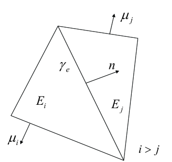
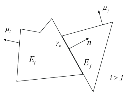
The following notations will be used in our further considerations. We set . The set of all edges of the partition is given by , where reprents the number of edges in the partition . The interior interface is then defined as the union of all common edges shared by elements of partition
| (2.2) |
The definition of the unit normal vector on each is related to the numbering of the elements in the partition, such that is defined outward with respect to the element with the highest index number. The normal vector is defined outward to each element individually. Within the setting above, the following reaction-diffusion problem is considered
| (2.3) | |||||
| (2.4) |
where is a real-valued function in and . For the sake of clarity in the notation, the jump and average operators on each are, respectively, defined as
| (2.5) |
where is the common edge(in 2D and interface in 3D) between two neighbouring elements.
2.2 The weak formulation of the problem (2.3)-(2.4)
The discontinuous Galerkin method is a class of finite element methods using completely discontinuous piecewise polynomial space for the numerical solution and the test functions. First, we introduce the following :
where
The norm of is defined as
| (2.6) | |||||
where . One can easily prove that norms and are equivalent. The parameter that is introduced here represents the minimum of all of the local orders of polynomial approximations in the partition . Notice that the parameters are greater than or equal to zero and that the subsequent norms in (2.6) are defined as
| (2.7) | |||||
| (2.8) |
where denotes the duality pairing in , namely,
| (2.9) |
And denotes the trace operator
Now, the choice for the space of test functions, , is the completion of with respect to the norm . The new discontinuous variational formulation, within this new function space setting, is then stated as follows:
| (2.10) |
where the bilinear form and linear form are defined as
| (2.11) | |||||
| (2.12) |
where and denote the jump and average operators, respectively.
Remark 2.1.
The formulation is closely related to the DG formulation by Oden, Babuska and Baumann [15]. Indeed, if we choose the subspace of of function with fluxes , then we again get the DG formulation of [15]. The only difference would then be the addition of the last term in (2.11). This term has been incorporated in [17, 14], where it is accompanied by another penalty term on the jumps of the function across the element interfaces. We replace the jumps by the jumps, in order to prove both continuity and Inf-Sup properties of the bilinear form with respect to the space , in which the norm is defined as .
2.3 The discrete problem
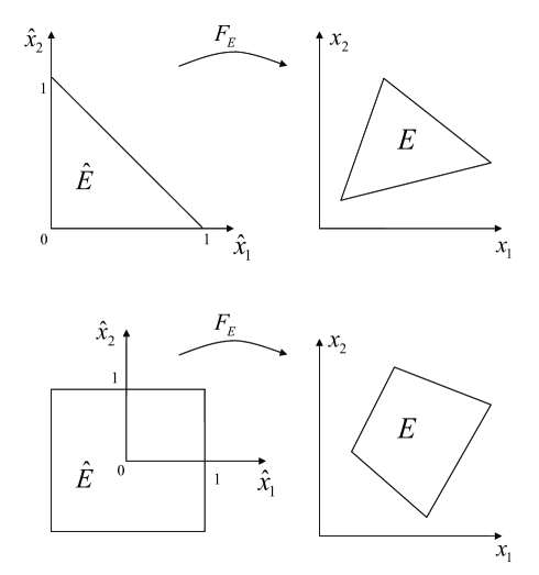
When implementing the DG methods, we have to compute integrals over volumes(such as triangles or quadrilaterals in 2D, terahedra or hexahedra in 3D) and faces(such as edges in 2D, triangles or quadrilaterals in 3D). It would be too costly to compute the integrals over each physical element in the mesh. A more economical and effective approach is to use a change of variables to obtain an integral on a fixed element, called the reference element. Let be a family of invertible maps defined for a partition such that every element is the image of acting on a reference element , as shown in Figure 2.
| (2.13) |
In the computational model, a finite-dimensional space of real-valued piecewise polynomial functions of degree is introduced, such that
| (2.14) |
is noted that a subspace of . Now, an approximation of is sought as the solution of the following discrete problem:
| (2.15) |
where the bilinear form is given by (2.11).
3 Inf-Sup condition on the discrete space
The following trace theorem is used to establish the Inf-Sup condition on the discrete space .
Lemma 3.1.
Let be characterized by an affine mapping (see section 2.3) and . Then there exists a constant , independent of , such that
| (3.1) |
One can find the proof of the lemma in [20].
Corollary 3.1.
Given a polynomial(degree ) , and the mapping between and is affine, then there exists such that
| (3.2) |
Proof.
Theorem 3.1.
Let be a family of affine invertible mappings. If , then there exists a , such that
| (3.5) |
here we can write
Proof.
By definition of the supremum, we get
| (3.6) |
By applying Corollary 3.1, it is clear that there exists , such that
| (3.7) | |||||
which completes the proof. ∎
4 Error estimation
In this section, we investigate the convergence properties of solution of (2.15). Let be the exact solution to the VBVP (2.10), then by using the linearity of , it follows easily that the approximation error is governed by
| (4.1) |
where is the residual functional. Note that, due to (2.15), the residual satisfies the following orthogonality property on ,
| (4.2) |
We start firstly by proving an interpolation theorem in the norm , secondly we need for our proof of the error estimate in this norm. Then we derives the convergence rates in the norm . Finally we prove an error estimate in the norm.
We introduce a family of interpolants , such that
Some results for the interpolation errors from the work of Babuska and Suri [5] will be needed.
Theorem 4.2.
For , there exists , independent of and and a sequence , such that
where .
By extending the local interpolant operators to zero outside of for every , we can define the global interpolant as follows
| (4.3) |
We define the notations as follows,
where
Theorem 4.3.
Let and , let the stabilization parameters and , and let the norm parameters , there exists , independent of , and such that the interpolation error can be bounded as follows
where
and where .
The norm in the space is defined as
Proof.
Theorem 4.4.
Proof.
Given the interpolation defined in (4.3). Note that and that the interpolation error . Consequently, using the triangle inequality, we obtain
| (4.4) |
Applying the discrete Inf-Sup condition of Theorem 3.1 and taking and , we obtain
Using the orthogonality property (4.2), the inequality can be rewritten as
Taking and , we have
Thus, returning to (4.4), we can conclude
With this choice of coefficients, we get for the parameters in Theorem 4.3
Hence, we finish the proof. ∎
Remark 4.1.
Since , the above theorem would imply suboptimal convergence rates for the error in the norm .
In the following, we derive optimal convergence rates for the error in the norm for . The decisive element in the proof is the use of a specific type of interpolants, that were introduced by Riviere et al [21]. The original estimates were them improved in [22, 18]. By using these interpolants, we succeed at proving optimal convergence rates for , but the convergence rates appear to be order lower than the one predicted in the previous section. So we succeed at improving the convergence rate, but not the rates.
We start our analysis by defining the following norm on ,
| (4.5) |
Lemma 4.1.
The bilinear form is continuous on with respect to the norm , i.e., there exists , such that
| (4.6) |
where is a constant, independent of and .
Next, we introduce an important inverse inequality (see [23]) between the spaces and for finite-dimensional functions .
Lemma 4.2.
Let the parameters in the norm be set as , then there exists a constant dependent of , such that
| (4.7) |
where denotes the piecewise average of
| (4.8) |
Similar to our proofs in the other sections, we need a theorem on the interpolation error in the norm . As mentioned previously, here we do not use the Babuska and Suri [5] interpolants but rather the interpolants proposed by Riviere et al [21].
Theorem 4.5.
Let , , there exists , independent of and , and interpolant , such that
| (4.9) |
and
where .
Again, by extending the corresponding local interpolant equal to zero outside of each , we can define a global interpolant on
| (4.10) |
Theorem 4.6.
Let be the interpolant of (4.10) and let the stabilization parameters and , then there exists , independent of , and such that the interpolation error can be bounded as follows
where
and where .
Proof.
Theorem 4.7.
Proof.
Given the interpolant in (4.10), using the triangle inequality, we can obtain
| (4.11) |
From (2.11) and (2.12), it follows that
| (4.12) |
Using the orthogonality property (4.2) and the linearity of , this can be rewritten as
| (4.13) |
where denotes the piecewise average (4.8) of . Now, applying Lemma 4.1 to the first term in the right hand side, we get
| (4.14) |
Applying the inverse inequality of Lemma 4.2, we can rewrite the above inequality as
| (4.15) |
As we shall now see, the term can be bounded in terms of as well, due to the special property (4.9) of the interpolant . By expanding the term , we get
Now, applying the property (4.9), gives
Back substitution of this result into (4.15) and (4.11), then yields
Next, recalling the interpolation Theorem 4.6, we get
Since , we know that and . ∎
Remark 4.2.
Now, we prove the error estimate in the norm. We will apply the Aubin-Nitsche lift technique used in the analysis of the classical finite element method to the DG method. First we introduce an important result (see [20]) as follows.
Theorem 4.8.
Let for . Let be an integer. There exists a constant independent of and and a function such that for all ,
| (4.16) |
We assume that the domain is convex and that the solution to the dual problem
belongs to with continuous dependence on ,
| (4.17) |
Then, we have
because of the regularity of we know that the jumps . Now subtracting the orthogonality property (4.2) from the equation above, we get
We choose , a continusous interpolant of of degree , and assume that such an interpolant exists. In this case, the first term is easily bounded using Cauchy-Schwarz inequality and the Theorem 4.8,
The rest terms except in the right hand side (4), yields
Therefore, by the Theorem 4.7 and using the bound (4.17), we obtain
Then, we have the following theorem:
Theorem 4.9.
Assume that Theorem 4.7 holds. Then there exists a constant independent of and , but dependent of , such that
where .
Remark 4.3.
For the results of Theorem 4.9, we can find that for the stabilization term of order and for , the convergence rates are of order and for and convergence, respectively.
5 Numerical results
For the 2D example problem, we consider the following VBVP, given on the unit square with prescribed Dirichlet boundary conditions on ,
| (5.1) |
Here we take , and the exact solution to this problem we choose is
| (5.2) |
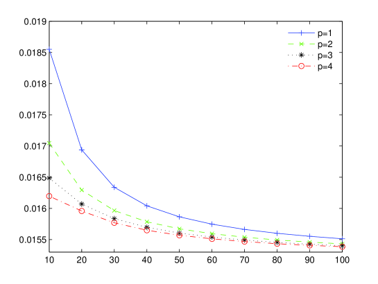
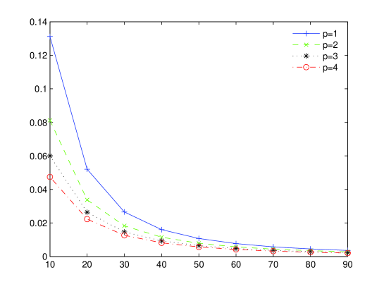
In the convergence analyses performed here, the orders of the norm and stabilization parameters are set equal to , i.e., taking . In Figure 3, the results are shown for the approximation error in the norm. Figure 4 shows the convergence rates with respect to the norm. And the rule of obtaining the rates is defined as
| (5.3) |
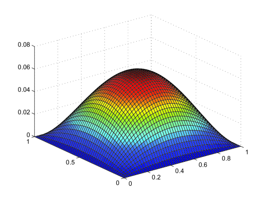
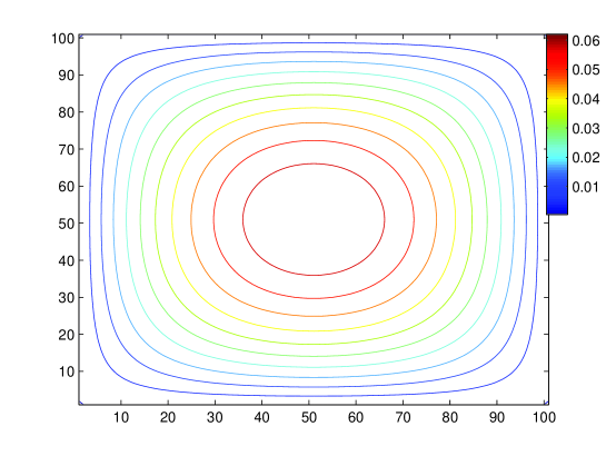
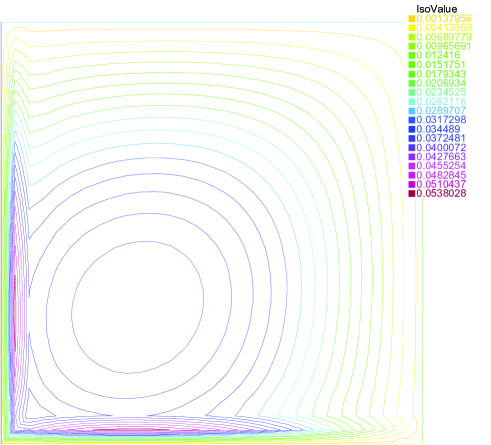
Figure 5 and 6 show the exact solution (5.2) and its contour figure, respectively. At last, the numerical solution is shown by using our method in Figure 7.
6 Conclusion
We introduce a new DG formulation and analyse the case of a two-dimensional reaction-diffusion problem with Dirichlet boundary conditions. The method is similar to the general DG method of [4, 15], but involves an extra stabilization term on the jumps of the fluxes across the element interfaces. In the work, we apply the conforming mesh as Figure 1 shows, but generally we can constrct elements as the Figure 8 shows, and the elements are even star-shaped as . Appliations of this type of element one can find in [11].
In addation, a new space setting is introduced. Instead of choosing the conventional , which is predominantly used in discontinuous Galerkin methods, we relax the constrains on the space and choose functions that are locally in and whose jumps in the fluxes across the element interfaces are in .
References
- [1] D.N. Arnold, An interior penalty finite element method with discontinuous elements, SIAM J.Numer. Anal., 19 (1982) 742-760.
- [2] D.N. Arnold, F. Brezzi, B. Cockburn, and D. Marini, Unified analysis of discontinuous Galerkin methods for elliptic problems, SIAM J. Numer. Anal., 39 (2001) 1749-1779.
- [3] I. Babuska, The finite element method with penalty, Math. Comput., 27 (1973) 221-228.
- [4] I. Babuska, C. Baumann, and J. Oden, A discontinuous hp-finite element method for diffusion problems: 1-D analysis, Comput. Appl. Math., 37 (1999) 103-122.
- [5] I. Babuska and M. Suri, The hp-version of the finite element method with Lagrangian multipliers, Mathematical Modelling and Numerical Mathematics, 21 (1987) 199-238.
- [6] I. Babuska and M. Zlamal, Nonconforming elements in the finit elements method with penalty, SIAM J. Numer. Anal., 10 (1973) 863-875.
- [7] F. Bassi and S. Rebay, A high-order accurate discontinuous finite element method for the numerical solution of the compressible Navier-Stokes equations, J. Comput. Phys., 131 (1997) 267-279.
- [8] F. Brezzi, G. Manzini, D. Marini, P. Pietra, and A. Russo, Discontinuous Galerkin approximations for elliptic problems, Numer. Methods Partial Differ. Eq., 16 (2000) 365-378.
- [9] P. Castillo, B. Cockburn, I. Perugia, and D. Schotzau, An a priori error analysis of the local discontinuous Galerkin method for elliptic problems, SIAM J. Numer. Anal., 38 (2000) 1676-1706.
- [10] B. Cockburn and C.W. Shu, The local discontinuous Galerkin finite element method for convection-diffusion systems, SIAM J. Numer. Anal., 35 (1998) 2440-2463.
- [11] V. Dolejsi, M. Feistauer and V. Sobotikova, Analysis of the discontinuous Galerkin method for nonlinear convection-diffusion problems, 194 (2005) 2709-2733.
- [12] J. Douglas, Jr. and T. Dupont, Interior penalty procedures for elliptic and parabolic Galerkin methods, Lecture Notes in Physics 58, Springer-Verlag, Berlin, 1976.
- [13] Z. Ge, J. Cao. A new variational formulation based on discontinuous Galerkin technique for a reaction-diffusion problem, preprint. arXiv:1204.4144v1.
- [14] T.J.R.Hughes, G.Engel, L. Mazzei and M.G. Larson, A comparison of discontinuous and continuous Galerkin methods based on error estimates, conservation, robustness and efficiency, Lecture Notes in Computational Science an Engineering, 11 (1999) 135-146.
- [15] J.T. Oden, I. Babuska and C.E. Baumann, A discontinuous hp finite element method for diffusion problem, J. Comput. Phys., 146 (1998) 491-519.
- [16] J. Oden and C.E. Baumann, A discontinuous hp finite element method for the Navier-Stokes equations, 10th. International Conference on Finite Element in Fluids, 1998.
- [17] P. Percell and M.F. Wheeler, A local residual finite element procedure for elliptic equations, SIAM J. Numer. Anal., 15 (1978) 705-714.
- [18] S. Prudhomme, F. Pascal, J.T. Oden and A. Romkes, A priori error estimates for the Baumann-Oden version of the discontinuous Galerkin method, Comptes Rendus de l’Academie des Sciences I, Numer. Anal., 322 (2001) 851-856.
- [19] W.H. Reed and T.R. Hill, Triangular mesh methods for the neutron transport equation, Tech. Report LA-UR-73-479, Los Alamos Scientific Laboratory, 1973.
- [20] B. Riviere. Discontinuous Galerkin Methods for Solving Elliptic and Parabolic Equations: Theory and Implementation, SIAM, Philadelphia, 2008.
- [21] B. Riviere, M.F. Wheeler and V. Girault, Improved enery estimates for interior penality, constrained and discontinuous Galerkin methods for elliptic problems. Part I, Computational Geosciences, 3 (1999) 337-360.
- [22] B. Riviere, M.F. Wheeler and V. Girault, A priori error estimates for finite element methods based on discontinuous approximation spaces for elliptic problems, SIAM J. Numer. Anal., 39 (2001) 902-931.
- [23] A. Romkes, S. Prudhomme and J.T. Oden. A priori error analyses of a stabilized discontinuous Galerkin method, Computers & Mathematics with Applications, 46 (2003) 1289-1311.
- [24] C. Schwab, P- and hp- finite element method: theory and applications in solid and fluid mechanics. Oxford University Press, New York, 1998.
- [25] M.F. Wheeler, An elliptic collocation-finite element method with interior penalities, SIAM J. Numer. Anal., 15 (1978) 152-161.