Strong Heegaard diagrams and strong L-spaces

Abstract.

We study a class of 3-manifolds called strong L-spaces, which by definition admit a certain type of Heegaard diagram that is particularly simple from the perspective of Heegaard Floer homology. We provide evidence for the possibility that every strong L-space is the branched double cover of an alternating link in the three-sphere. For example, we establish this fact for a strong L-space admitting a strong Heegaard diagram of genus two via an explicit classification. We also show that there exist finitely many strong L-spaces with bounded order of first homology; for instance, through order eight, they are connected sums of lens spaces. The methods are topological and graph theoretic. We discuss many related results and questions.

1. Introduction

The purpose of this paper is to study a family of $3$-manifolds called strong L-spaces. These manifolds are defined by a combinatorial condition on Heegaard diagrams, and they arise naturally in the context of Heegaard Floer homology.

In its simplest form, the Heegaard Floer homology [OSz3Manifold] of a closed, oriented $3$-manifold $Y$ is a finitely generated abelian group $\widehat{\operatorname{HF}}(Y)$, defined as follows. We present $Y$ by means of a Heegaard diagram $H$, consisting of a closed, oriented surface $S$ of genus $g$ and two disjoint unions of embedded circles in $S$, $\alpha=\alpha_{1}\cup\dots\cup\alpha_{g}$ and $\beta=\beta_{1}\cup\dots\cup\beta_{g}$, each of which spans a $g$-dimensional subspace of $H_{1}(S;\mathbb{Z})$ and which intersect each other transversally. To such a diagram, we associate a chain complex $\widehat{\operatorname{CF}}(H)$, which is freely generated by the set $\SS(H)$ of unordered $g$-tuples of points in $S$ with one point on each $\alpha$ circle and one point on each $\beta$ circle. By adapting the machinery of Lagrangian Floer homology, Ozsváth and Szabó define a differential $\partial$ on $\widehat{\operatorname{CF}}(H)$ that also depends on some additional choices of analytic data. They prove that the homology $H_{*}(\widehat{\operatorname{CF}}(H),\partial)$ depends only on the $3$-manifold $Y$ and not on the specific choice of Heegaard diagram or analytic data. This homology group is denoted $\widehat{\operatorname{HF}}(Y)$.

Define the determinant $\det(Y)$ of a $3$-manifold $Y$ to be the order of $H_{1}(Y;\mathbb{Z})$ if this group is finite (i.e. when $Y$ is a rational homology sphere) and $0$ otherwise. With respect to a natural $\mathbb{Z}/2$–grading, the Euler characteristic of $\widehat{\operatorname{CF}}(Y)$ is equal to $\det(Y)$ [OSzProperties]. As a result, for any Heegaard diagram $H$ presenting $Y$, we have

(1) $$\left\lvert\SS(H)\right\rvert=\operatorname{rank}\widehat{\operatorname{CF}}(H)\geq\operatorname{rank}\widehat{\operatorname{HF}}(Y)\geq\det(Y).$$

If $\det(Y)\neq 0$ and $\widehat{\operatorname{HF}}(Y)$ is free abelian of rank $\det(Y)$, $Y$ is called an L-space. In view of (1), such manifolds can be seen as having the simplest possible Heegaard Floer homology. Examples of L-spaces include $S^{3}$, lens spaces (whence the name), all manifolds with finite fundamental group, and branched double covers of non-split alternating (or, more generally, quasi-alternating) knots and links in $S^{3}$ [OSzDouble]. The classification of L-spaces is one of the major outstanding questions in Heegaard Floer theory. For instance, it is conjectured that a rational homology sphere $Y$ is an L-space if and only if $\pi_{1}(Y)$ is not left-orderable. This conjecture is known to hold (at least mod torsion) for many classes of manifolds, including all geometric, non-hyperbolic manifolds [BoyerGordonWatson].

The minimum size of $\SS(H)$, ranging over all Heegaard diagrams $H$ for a rational homology sphere $Y$, may be viewed as a measure of the topological complexity of $Y$. This quantity is called the simultaneous trajectory number of $Y$ and is denoted $M(Y)$ [OSzProperties, Section 1.2]. Both $\det(Y)$ and $\operatorname{rank}(\widehat{\operatorname{HF}}(Y))$ provide lower bounds on $M(Y)$ by (1). The second author and Lewallen [LevineLewallen] introduced the following definition:

Definition 1.1.

A closed, oriented $3$-manifold $Y$ is called a strong L-space if $M(Y)=\det(Y)$. A Heegaard diagram $H$ for $Y$ for which $\left\lvert\SS(H)\right\rvert=\det(Y)$ is called a strong Heegaard diagram.

By (1), a strong L-space is an L-space. In view of the conjecture mentioned above, the second author and Lewallen proved that the fundamental group of a strong L-space is not left-orderable [LevineLewallen]. As a simple direct consequence, a strong L-space cannot admit an ${\mathbb{R}}$-covered taut foliation. In fact, Ozsváth and Szabó established the much deeper result that an L-space does not admit any co-orientable taut foliation [KazezRoberts, OSzGenus].

Our motivating problem is to describe the homeomorphism types of strong L-spaces and strong Heegaard diagrams. As we shall see, the condition of being a strong L-space is quite restrictive, more so than being an L-space. For instance, the only strong L-space with determinant $1$ is $S^{3}$, so the Poincaré homology sphere is an L-space but not a strong L-space [OSzProperties, LevineLewallen].

The standard genus-$1$ Heegaard diagram for a lens space $L(p,q)$ (consisting of a single $\alpha$ curve and a single $\beta$ curve on a torus, intersecting $p$ times) is clearly a strong diagram, so lens spaces are strong L-spaces. A broader source of examples derives from work of the first author, who showed that the double cover of $S^{3}$ branched along a non-split alternating link is a strong L-space [GreeneSpanning, Corollary 3.5]. Note that these spaces subsume lens spaces, which are branched double covers of two-bridge links, although the strong diagrams for these spaces in [GreeneSpanning] do not have genus $1$. Although we can generate many families of strong Heegaard diagrams, we were unable to produce any new examples of strong L-spaces besides the ones just mentioned. Indeed, our main results support an affirmative answer to the following question:

Question 1.2.

Is every strong L-space the branched double cover of an alternating link in $S^{3}$?

As a first approach to Question 1.2, recall that the determinant of a link $L\subset S^{3}$ is the absolute value of its (single-variable) Alexander polynomial evaluated at $-1$: $\det(L)=\left\lvert\Delta_{L}(-1)\right\rvert$. Let $\Sigma(L)$ denote the double cover of $S^{3}$ branched over $L$. Then $\det(L)=\det(\Sigma(L))$, in part justifying our terminology. A classical theorem of Bankwitz and Crowell asserts that there exist finitely many alternating links of bounded determinant [BankwitzAlternating, CrowellNonalternating]. Therefore, an affirmative answer to Question 1.2 would imply the same about strong L-spaces. We deduce this fact directly as a corollary of the following result, which we prove using topological and graph-theoretic methods:

Theorem 1.3.

There exist finitely many rational homology spheres with bounded simultaneous trajectory number.

Corollary 1.4.

There exist finitely many strong L-spaces with bounded determinant. ∎

By contrast, there exist infinitely many irreducible L-spaces with the same determinant. Reducible examples are easy to exhibit, since Heegaard Floer homology satisfies a Künneth principle for connected sums. Thus, for example, the connected sum of any L-space with arbitrarily many copies of the Poincaré sphere is an L-space with the same determinant. For irreducible examples, the Seifert fibered spaces of type $(2,2,n)$ all have determinant $4$ and finite fundamental group, so they are L-spaces. (It is unknown whether there exist infinitely many irreducible L-spaces with determinant less than $4$.) Additionally, the first author and Watson [GreeneWatsonQA] gave an infinite family of hyperbolic manifolds with determinant $25$ that are L-spaces mod torsion.

Using similar techniques to those in the proof of Theorem 1.3, we prove:

Theorem 1.5.

If $Y$ is a strong L-space with $\det(Y)\leq 8$, then $Y$ is the branched double cover of an alternating link. Specifically, $Y$ is a connected sum of lens spaces.

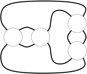
Figure 1. Diagram of the link $L(a_{1},a_{2},a_{3},a_{4})$, $a_{1},a_{2},a_{3},a_{4}\in\mathbb{Q}\cup\{1/0\}$.

In another direction towards Question 1.2, we describe all strong L-spaces that admit strong Heegaard diagrams of genus 2. For $a_{1},a_{2},a_{3},a_{4}\in\mathbb{Q}\cup\{1/0\}$, let $L(a_{1},a_{2},a_{3},a_{4})$ denote the link presented by the the diagram in Figure 1, where the four balls are filled in with the rational tangles specified by $a_{1},a_{2},a_{3},a_{4}$ (see Section 5.2). Note that the diagram is alternating iff all $a_{i}$ have the same sign, where $0/1$ and $1/0$ are considered to have both signs. Setting $a_{1}=a_{2}=a_{3}=a_{4}=\pm 1$ results in the minimal diagram $D$ of the figure eight knot, so the diagram can be regarded as substituting arbitrary rational tangles for the crossings in $D$. The branched double cover $\Sigma(L(a_{1},a_{2},a_{3},a_{4}))$ is either (1) a connected sum of one or two genus-1 manifolds, (2) a small Seifert fibered space, or (3) a graph manifold whose JSJ decomposition consists of two Seifert fibered spaces over $D^{2}$ with two exceptional fibers.

Theorem 1.6.

Let $Y$ be a strong L-space that admits a strong Heegaard diagram of genus $2$. Then for some $a_{1},\dots,a_{4}\in\mathbb{Q}\cup\{1/0\}$ of the same sign, $Y\cong\Sigma(L(a_{1},a_{2},a_{3},a_{4}))$. In particular, $Y$ is the branched double cover of an alternating link in $S^{3}$.

Usui [UsuiSmoothing1, UsuiSmoothing2] has obtained similar results.

A key ingredient for proving Theorems 1.3 and 1.6 is Proposition 3.1, which implies that every strong L-space admits a Heegaard diagram $H$ that is both strong and 1-extendible. In such a diagram, the signs with which the $\alpha$ and $\beta$ curves may intersect are highly constrained: all points of intersection between any two curves have the same sign, and the associated intersection matrix is a Pólya matrix (see Section 2). Theorems 1.3 and 1.5 then follow from topological and graph theoretic arguments, and their proofs appear in Section 4. To prove Theorem 1.6, we show in Section 5 that every strong, 1-extendible Heegaard diagram of genus 2 has a standard form, which coincides precisely with a particular class of Heegaard diagrams for $\Sigma(L(a_{1},a_{2},a_{3},a_{4}))$ for $a_{1},a_{2},a_{3},a_{4}$ of the same sign.

In Section LABEL:sec:_simpleknots, we prove some results concerning Floer simple knots in strong L-spaces that admit genus-2 strong diagrams. The existence of such knots has applications to Dehn surgery and minimal genus problems. In Section LABEL:sec:_waves, we discuss the connections between strong L-spaces and other notions pertaining to Heegaard splittings. We close in Section LABEL:sec:_questions with several questions motivated by the present work.

Acknowledgments

We extend our foremost thanks to John Luecke, who had a great influence on this work. We also warmly thank Cameron Gordon, Sam Lewallen, and Nathan Dunfield for enjoyable, stimulating discussions.

2. Preliminaries

For an oriented, properly embedded curve $\alpha$ in a surface (possibly with boundary), let $-\alpha$ denote the same curve with the opposite orientation, and for any integer $n$, let $n\alpha$ denote a multi-curve obtained by taking $|n|$ parallel copies of $\operatorname{sgn}(n)\alpha$. For oriented multi-curves $\alpha$ and $\beta$ that meet transversally, let $\alpha+\beta$ denote an oriented multi-curve obtained from $\alpha\cup\beta$ by forming the oriented resolution at every point of $\alpha\cap\beta$. Note that $n\alpha$ and $\alpha+\beta$ specify unique multi-curves up to isotopy. For oriented multi-curves $\alpha,\beta$ in an oriented surface $S$ that meet transversally, write $\alpha\cdot\beta$ for their algebraic intersection number and $\left\lvert\alpha\cap\beta\right\rvert$ for their geometric intersection number. The multi-curves $\alpha$ and $\beta$ intersect coherently if all intersection points have the same sign, i.e., if $\left\lvert\alpha\cdot\beta\right\rvert=\left\lvert\alpha\cap\beta\right\rvert$.

A Heegaard diagram $H$ consists of a surface $S$, a basepoint $z$, two collections of attaching curves $\alpha=\alpha_{1}\cup\cdots\cup\alpha_{g}$ and $\beta=\beta_{1}\cup\cdots\cup\beta_{g}$ specifying a pair of handlebodies, and a choice $o$ of orientation on $S$ and each $\alpha$ and $\beta$ curve:

$$(S,z,\alpha,\beta,o).$$

Henceforth, we generally suppress reference to the basepoint $z$ and orientation $o$, and simply refer to the diagram as $(S,\alpha,\beta)$.

Let $\operatorname{Sym}^{g}(S)$ denote the $g^{\text{th}}$ symmetric power of $S$, the quotient of $S^{\times g}$ by the action of the symmetric group on $g$ letters. It is a $2g$-dimensional manifold. Let $\mathbb{T}_{\alpha}$ (resp. $\mathbb{T}_{\beta}$) be the image in $\operatorname{Sym}^{g}(S)$ of $\alpha_{1}\times\cdots\times\alpha_{g}$ (resp. $\mathbb{T}_{\beta}$); this is an embedded $g$-dimensional torus. The tori $\mathbb{T}_{\alpha}$ and $\mathbb{T}_{\beta}$ intersect transversally in a finite number of points; let $\SS(H)=\mathbb{T}_{\alpha}\cap\mathbb{T}_{\beta}$. A point of $\SS(H)$ is a tuple ${{\bf x}}=(x_{1},\dots,x_{g})$, where $x_{i}\in\alpha_{i}\cap\beta_{\sigma_{{{\bf x}}}(i)}$, for some permutation $\sigma_{{\bf x}}$. Elements of $\SS(H)$ are generators of the group $\widehat{\operatorname{CF}}(H)$ discussed above.

For each $x\in\alpha_{i}\cap\beta_{j}$, let $\eta(x)\in\{\pm 1\}$ denote the local sign of intersection of $\alpha_{i}$ with $\beta_{j}$ at $x$. For ${{\bf x}}=(x_{1},\dots,x_{g})\in\SS(H)$, the local sign of intersection of $\mathbb{T}_{\alpha}$ and $\mathbb{T}_{\beta}$ is given by

$$\eta({{\bf x}})=\operatorname{sign}(\sigma_{{\bf x}})\prod_{i=1}^{g}\eta(x_{i})$$

where $\operatorname{sign}(\sigma_{{\bf x}})\in\{\pm 1\}$ is the signature of the permutation $\sigma_{{\bf x}}$. Note that changing the orientation of $S$ or a single $\alpha$ or $\beta$ curve negates $\eta({{\bf x}})$ for all ${{\bf x}}\in\SS(H)$.

The intersection matrix $M(H)$ is the $g\times g$ matrix of integers whose $(i,j)$ entry is

$$m_{i,j}=\alpha_{i}\cdot\beta_{j}=\sum_{x\in\alpha_{i}\cap\beta_{j}}\eta(x).$$

Since $M(H)$ is a presentation matrix for $H_{1}(Y)$, we have $\det(Y)=\left\lvert\det(M(H))\right\rvert$, which explains our choice of terminology. The permutation expansion of the determinant gives:

$$\det(M(H)) =\sum_{\sigma}\operatorname{sign}(\sigma)m_{1,\sigma(1)}\cdots m_{g,\sigma(g)}$$

$$=\sum_{\sigma}\operatorname{sign}(\sigma)\sum_{\begin{subarray}{c}\{(x_{1},\dots,x_{g})\mid\\ x_{i}\in\alpha_{i}\cap\beta_{\sigma(i)}\}\end{subarray}}\prod_{i=1}^{g}\eta(x_{i})$$

$$=\sum_{{{\bf x}}\in\SS(H)}\eta({{\bf x}}).$$

In particular, we see that

$$\left\lvert\SS(H)\right\rvert\geq\det(Y),$$

as noted in the Introduction. The following two lemmas are immediate:

Lemma 2.1.

$H$ is a strong Heegaard diagram if and only if all generators in $\SS(H)$ have the same sign. ∎

Lemma 2.2.

If $H$ is a strong Heegaard diagram, and some generator in $\SS(H)$ includes a point of $\alpha_{i}\cap\beta_{j}$, then $\alpha_{i}$ and $\beta_{j}$ intersect coherently. ∎

We call a Heegaard diagram $H$ coherent if all pairs of $\alpha$ and $\beta$ curves intersect coherently. As we shall see, the fact that (many of) the curves in a strong Heegaard diagram intersect coherently will be vital to our classification results. However, a strong diagram need not be coherent. For instance, if $H$ is a genus-2 Heegaard diagram in which the intersections $\alpha_{1}\cap\beta_{1}$ and $\alpha_{2}\cap\beta_{2}$ are coherent and non-empty, while $\alpha_{1}\cap\beta_{2}=\emptyset$, then $H$ is strong irrespective of the signs of points in $\alpha_{2}\cap\beta_{1}$, since these points are not included in elements of $\SS(H)$. Such a diagram can be obtained by taking the connected sum of two standard Heegaard diagrams for lens spaces and isotoping the $\alpha$ curve of one summand so that it intersects the $\beta$ curve of the other summand. However, Proposition 3.1 below will enable us to restrict our attention to coherent Heegaard diagrams.

Given a Heegaard diagram $H$, the intersection graph $G(H)$ is the bipartite graph with vertex set $A\sqcup B$, where $A=\{a_{1},\dots,a_{g}\}$ and $B=\{b_{1},\dots,b_{g}\}$, and for which the set of edges joining $a_{i}$ and $b_{j}$ is $\{e_{x}\mid x\in\alpha_{i}\cap\beta_{j}\}$. Note that $\SS(H)$ is in natural one-to-one correspondence with the set of perfect matchings of $G(H)$. The degree of a vertex $v$ in a graph $G$ is the number of edges in $G$ with an endpoint at $v$. Write $\delta(G)$ for the minimum vertex degree in $G$, and write $\delta(H)=\delta(G(H))$. A graph $G$ is $k$-extendible if any $k$-tuple of disjoint edges extends to a perfect matching of $G$. A Heegaard diagram $H$ is $k$-extendible if its intersection graph $G(H)$ is. In particular, $H$ is $1$-extendible if every point $x\in\alpha\cap\beta$ is contained in a generator ${{\bf x}}\in\SS(H)$. As an immediate consequence of the previous two lemmas, we have:

Lemma 2.3.

A strong, $1$-extendible Heegaard diagram is coherent. ∎

For a strong diagram $H$, the combinatorics of $M(H)$ and $G(H)$ are expressed by the closely related concepts of Pólya matrices and Pfaffian orientations, respectively. A Pólya matrix is a $g\times g$ square matrix $M=(m_{i,j})$ for which all non-zero terms in the expansion

$$\det(M)=\sum_{\sigma}\operatorname{sign}(\sigma)m_{1,\sigma(1)}\cdots m_{g,\sigma(g)}$$

come with the same sign. Equivalently, if we write $\left\lvert M\right\rvert$ for the matrix $(\left\lvert m_{i,j}\right\rvert)$ and

$$\operatorname{per}(N)=\sum_{\sigma}n_{1,\sigma(1)}\cdots n_{g,\sigma(g)}$$

for the permanent of a $g\times g$ square matrix $N=(n_{i,j})$, then $M$ is a Pólya matrix if

$$\left\lvert\det(M)\right\rvert=\operatorname{per}(\left\lvert M\right\rvert).$$

We refer to [vy:pfaffian] for the definition of a Pfaffian orientation.

Proposition 2.4.

The following are equivalent conditions on a coherent Heegaard diagram $H$: (1) $H$is strong, (2) $M(H)$is a Pólya matrix, and (3) $G(H)$has a Pfaffian orientation.

Proof.

The equivalence of (1) and (2) is the effective content of Lemma 2.1. The equivalence of (2) and (3) follows from [vy:pfaffian]. ∎

The sign pattern of the entries of a Pólya matrix is highly constrained. This fact plays a key role in the proof that the fundamental group of a strong L-space is not left-orderable [LevineLewallen]. Pólya matrices obey a deep structure theorem due independently to McCuaig [mccuaig:polya] and Robertson, Seymour, and Thomas [rst:polya]. We apply a result of their work in Section LABEL:subsec:_reducibility.

3. Extendibility

The purpose of this section is to show that every rational homology sphere admits a 1-extendible Heegaard diagram attaining its simultaneous trajectory number. In particular, every strong L-space admits a 1-extendible, strong Heegaard diagram. This result is very useful in the subsequent sections. The technical statement is as follows:

Proposition 3.1.

Let $H$ be a doubly-pointed Heegaard diagram for a rational homology sphere. Then there exists a sequence of handleslides and isotopies in the complement of the basepoints that transforms $H$ into a 1-extendible Heegaard diagram $H^{\prime}$ such that $\left\lvert\SS(H)\right\rvert=\left\lvert\SS(H^{\prime})\right\rvert$. In particular, if $H$ is strong, then so is $H^{\prime}$.

Corollary 3.2.

A rational homology sphere $Y$ admits a 1-extendible Heegaard diagram $H$ for which $\left\lvert\SS(H)\right\rvert=M(Y)$. ∎

To prove Proposition 3.1, we begin by establishing a simple criterion to recognize that a given Heegaard diagram can be converted into a reducible one by a sequence of isotopies and handleslides. In order to state it in a sharp form, we require a little notation and background concerning Heegaard diagrams and presentations of the fundamental group.

Given any free group $F^{z}=\langle z_{1},\dots,z_{g}\rangle$ and a value $1\leq k\leq g$, we obtain groups

$$F^{z}_{\leq k}=\langle z_{1},\dots,z_{k}\rangle,\quad F^{z}_{k}=\langle z_{k}\rangle,\quad F^{z}_{\geq k}=\langle z_{k},\dots,z_{g}\rangle,$$

and projections from $F^{z}$ to each. For any word $w\in F^{z}$, let

$$w_{\leq k}=w_{<k+1},\quad w_{k},\quad\text{and}\quad w_{\geq k}=w_{>k-1},$$

denote the respective images of $w$ under these projections; each of them is a subword of $w$. In a similar spirit, for a collection of curves $\gamma_{1},\dots,\gamma_{g}$, we define

$$\gamma_{\leq k}=\gamma_{<k+1}=\gamma_{1}\cup\cdots\cup\gamma_{k}\quad\text{and}\quad\gamma_{>k}=\gamma_{k+1}\cup\cdots\cup\gamma_{g}.$$

Let $H=(S,\alpha,\beta)$ denote a Heegaard diagram that presents a 3-manifold $Y$. Form the free group $F^{x}=\langle x_{1},\dots,x_{g}\rangle$. Choose a point $p_{i}\in\alpha_{i}$ disjoint from $\beta$ and traverse a full loop around $\alpha_{i}$ starting at $p_{i}$. For each intersection point between $\alpha_{i}$ and $\beta_{j}$ with sign $\epsilon$, record the term $x_{j}^{\epsilon}$. The product of these terms, in order from left to right, yields a word $w_{\beta}(\alpha_{i})\in F_{x}$. Observe that a different choice of $p_{i}$ will result in the same word up to cyclic equivalence. As a result, we regard $w_{\beta}(\alpha_{i})$ and its subwords up to cyclic equivalence. The group $\pi_{1}(Y)$ admits the presentation $F^{x}/\langle w_{\beta}(\alpha_{1}),\dots,w_{\beta}(\alpha_{g})\rangle$. In an analogous manner, we define the free group $F^{y}=\langle y_{1},\dots,y_{g}\rangle$, associate a cyclic word $w_{\alpha}(\beta_{j})$ in $y_{1},\dots,y_{g}$ to each curve $\beta_{j}$, and obtain the presentation $F^{y}/\langle w_{\alpha}(\beta_{1}),\dots,w_{\alpha}(\beta_{g})\rangle$ for $\pi_{1}(Y)$.

Lemma 3.3.

Suppose that $H=(S,\alpha,\beta,z_{1},z_{2})$ is a doubly-pointed genus-$g$ Heegaard diagram for a rational homology sphere $Y$, and for some $0<k<g$,

$$\alpha_{\leq k}\cap\beta_{>k}=\emptyset.$$

Then it is possible to perform handleslides and isotopies in the complement of $z_{1}$ and $z_{2}$ to produce a Heegaard diagram $H^{\prime}=(S,\alpha^{\prime},\beta^{\prime},z_{1},z_{2})$ such that $\left\lvert\SS(H)\right\rvert=\left\lvert\SS(H^{\prime})\right\rvert$,

$$w_{\beta^{\prime}}(\alpha_{i}^{\prime})=w_{\beta}(\alpha_{i})_{\leq k},\quad w_{\alpha^{\prime}}(\beta_{j}^{\prime})=w_{\alpha}(\beta_{j})_{\leq k},\quad\forall\,i,j\leq k,$$

and

$$w_{\beta^{\prime}}(\alpha_{i}^{\prime})=w_{\beta}(\alpha_{i})_{>k},\quad w_{\alpha^{\prime}}(\beta_{j}^{\prime})=w_{\alpha}(\beta_{j})_{>k},\quad\forall\,i,j>k.$$

In particular, $\alpha_{\leq k}^{\prime}\cap\beta_{>k}^{\prime}=\alpha_{>k}^{\prime}\cap\beta_{\leq k}=\emptyset$, while there is an identification $\alpha_{i}^{\prime}\cap\beta_{j}^{\prime}=\alpha_{i}\cap\beta_{j}$ preserving local signs of intersection when $i,j\leq k$ or $i,j>k$. Thus, $H^{\prime}$ is reducible with summands $H_{1}=(S_{\leq k},\alpha_{\leq k}^{\prime},\beta_{\leq k}^{\prime})$ and $H_{2}=(S_{>k},\alpha_{>k}^{\prime},\beta_{>k}^{\prime})$. If $H$ is strong, then so are $H_{1}$ and $H_{2}$.

Remark 3.4.

Some restriction on $Y$ or $H$ is necessary in order to guarantee the conclusion of Lemma 3.3. For example, take $Y=S^{1}\times S^{2}$ (so $b_{1}(Y)>0$), consider its standard genus-$1$ Heegaard diagram with no intersection points, and stabilize the diagram once. Label the curves in the resulting diagram so that $\alpha_{1}\cap\beta_{2}=\emptyset$. The conclusion of Lemma 3.3 in this case (with $k=1$) would produce a genus-$2$ Heegaard diagram in which each pair of curves is disjoint, but such a diagram must present $\#^{2}(S^{1}\times S^{2})\neq Y$, a contradiction.

Proof of Lemma 3.3.

Recall that $H_{1}(Y;\mathbb{Z})\cong H_{1}(S;\mathbb{Z})/\langle[\alpha_{1}],\dots,[\alpha_{g}],[\beta_{1}],\dots,[\beta_{g}]\rangle.$ Since $Y$ is a rational homology sphere, it follows that the classes $[\alpha_{1}],\dots,[\alpha_{g}],[\beta_{1}],\dots,[\beta_{g}]$ are linearly independent in $H_{1}(S;\mathbb{Z})$. In particular, $\alpha_{1},\dots,\alpha_{k},\beta_{k+1},\dots,\beta_{g}$ are $g$ disjoint curves representing linearly independent classes in $H_{1}(S;\mathbb{Z})$. It follows that $S\smallsetminus(\alpha_{\leq k}\cup\beta_{>k})$ is a $2g$-punctured sphere. As a result, there exists an unoriented curve $\gamma\subset S$, unique up to isotopy, with a regular neighborhood $N(\gamma)$ that separates $S$ into subsurfaces $\overline{S}_{\leq k},\overline{S}_{>k}$ such that $\{z_{1}\}\cup\alpha_{\leq k}\subset\overline{S}_{\leq k}$ and $\{z_{2}\}\cup\beta_{>k}\subset\overline{S}_{>k}$. See Figure 2.

$\alpha_{1}$ at 112 260 $\alpha_{2}$ at 195 274 $\alpha_{3}$ at 281 286 $\beta_{4}$ at 128 98 $\beta_{5}$ at 250 103 $\overline{S}_{\leq 3}$ [bl] at 309 301 $\overline{S}_{>3}$ [tl] at 309 56 $z_{1}$ [l] at 183 344 $z_{2}$ [l] at 183 13 $\gamma$ [tl] at 294 159

Figure 2. A cut-open Heegaard diagram as in the proof of Lemma 3.3, with $k=3$ and $g=5$.

The space $N(\gamma)\cup\overline{S}_{>k}\smallsetminus\beta_{>k}$ is a $2(g-k)$-punctured disk, and $N(\gamma)\cap\overline{S}_{\leq k}$ is a collar neighborhood of its boundary. We radially isotope $\beta_{\leq k}\cap(N(\gamma)\cup\overline{S}_{>k})$ away from $z_{2}$ and into $N(\gamma)\cap\overline{S}_{\leq k}$, permitting arcs to pass over punctures in the process. Passing an arc over a puncture corresponds to a handleslide in $S$, so we may interpret this process as a sequence of isotopies and handleslides of $\beta_{\leq k}$ over $\beta_{>k}$ in $S$ which is the identity outside of $N(\gamma)\cup\overline{S}_{>k}\smallsetminus\{z_{2}\}$. The resulting collection of curves $\beta_{\leq k}^{\prime}$ supported in $\overline{S}_{\leq k}$ has the property that $w_{\alpha}(\beta_{j}^{\prime})_{\leq k}=w_{\alpha}(\beta_{j})_{\leq k}$ for all $j\leq k$, since $\alpha_{\leq k}\cap\beta_{>k}=\emptyset$ and the handleslides do not change the intersections of $\beta_{\leq k}$ with $\alpha_{\leq k}$. Similarly, we isotope and handleslide the curves $\alpha_{>k}$ over $\alpha_{\leq k}$ in $N(\gamma)\cup\overline{S}_{\leq k}\smallsetminus\{z_{1}\}$ to get curves $\alpha_{>k}^{\prime}$ supported in $\overline{S}_{>k}$ and such that $w_{\beta^{\prime}}(\alpha_{i}^{\prime})_{>k}=w_{\beta^{\prime}}(\alpha_{i})_{>k}$ for all $i$. Lastly, we define $\alpha_{i}^{\prime}=\alpha_{i}$ for $i=1,\dots,k$ and $\beta_{j}^{\prime}=\beta_{j}$ for $j=k+1,\dots,g$.

The preceding remarks and the fact that $\beta_{\leq k}^{\prime}\cap\alpha_{>k}^{\prime}=\emptyset$ yield the stated conclusions about $w(\alpha_{i}^{\prime})$ and $w(\beta_{j}^{\prime})$. Capping off $\overline{S}_{\leq k}$ and $\overline{S}_{>k}$ along $\gamma$ results in the surfaces $S_{\leq k}$ and $S_{>k}$ required by the Lemma. Finally, note that there exists a natural bijection between $\SS(H)$ and $\SS(H^{\prime})$, since a generator in $\SS(H)$ cannot use any element of $\alpha_{>k}\cap\beta_{\leq k}$. In particular, if $H$ is strong, then so is $H^{\prime}$. ∎

Proof of Proposition 3.1.

We proceed by induction on $g(H)$. For $g(H)=1$ the assertion is trivial, so we proceed to the induction step. By a theorem of Hetyei, a bipartite graph $G$ with bipartition $(A,B)$ is 1-extendible iff for every subset $T\subset A$, the set of neighbors of $T$ in $B$ has cardinality at least $\max\{|B|,|A|+1\}$ [hetyei], [LovaszPlummerBook, Theorem 4.1.1]. Since $G(H)$ contains a perfect matching, it is 0-extendible. Assume that it is not 1-extendible. Then there exists some proper, non-empty subset $T\subset A$ such that $T$ has exactly $|T|$ neighbors in $B$. In other words, there exist some $k$ $\alpha$ circles that are disjoint from some $(g-k)$ $\beta$ circles, where $1\leq k<g$. Thus, Lemma 3.3 implies that there exists a sequence of handleslides and isotopies which transform $H$ into a reducible diagram $H^{\prime}$, and which is strong provided that $H$ is. By induction on the genera of the summands of $H^{\prime}$, the statement of the Proposition follows. ∎

A simple induction using Lemma 3.3 establishes the following corollary:

Corollary 3.5.

If a strong diagram has an upper triangular intersection matrix, then it presents a connected sum of lens spaces. ∎

4. Finiteness results

In this section, we prove Theorem 1.3, which asserts that there exist finitely many rational homology spheres with bounded simultaneous trajectory number, and Theorem 1.5, which classifies the strong L-spaces with determinant up to 8.

Lemma 4.1.

Let $H$ be a Heegaard diagram for a rational homology sphere. Suppose that $H$ contains an attaching curve that has $m\geq 1$ intersection points with another attaching curve and at most one other intersection point. Then there exists a sequence of isotopies and handleslides converting $H$ into a 1-extendible Heegaard diagram $H_{1}\#H_{2}$ with $g(H_{1})=1$, $\left\lvert\SS(H_{1})\right\rvert=m$, and $\left\lvert\SS(H)\right\rvert=\left\lvert\SS(H_{1}\#H_{2})\right\rvert$. If $H$ is strong, then so are $H_{1}$ and $H_{2}$.

Proof.

Without loss of generality, assume that $\alpha_{1}$ has $m\geq 1$ intersection points with $\beta_{1}$. If $\alpha_{1}$ meets only $\beta_{1}$, then the result follows directly from Lemma 3.3 and induction on the genus, as in the proof of Proposition 3.1. Suppose instead that $\alpha_{1}$ meets another curve $\beta_{2}$. Label the intersection points along $\alpha_{1}$ consecutively by $p_{1},\dots,p_{m}\in\beta_{1}$ and $q\in\beta_{2}$. Perform $m$ consecutive handleslides of $\beta_{1}$ over $\beta_{2}$, guided along the oriented $\alpha_{1}$-arc from $p_{i}$ to $q$ for $i=m,\dots,1$ in turn. Let $\beta_{1}^{\prime}$ denote the resulting curve and $H^{\prime}$ the resulting Heegaard diagram. Observe that $\alpha_{1}$ has a single intersection point in $H^{\prime}$. Applying Lemma 3.3 and induction on the genus to $H^{\prime}$ establishes the existence of handleslides and isotopies converting $H^{\prime}$ into a 1-extendible Heegaard diagram of the required form with the property that $\left\lvert\SS(H^{\prime})\right\rvert=\left\lvert\SS(H_{1}\mathbin{\#}H_{2})\right\rvert$.

It remains to establish that $\left\lvert\SS(H^{\prime})\right\rvert=\left\lvert\SS(H)\right\rvert$. To do so, we exhibit a bijection between the perfect matchings in $G(H^{\prime})$ and $G(H)$. Let $G^{\prime}\subset G(H)$ denote the subgraph obtained by removing the $m$ edges between $a_{1}$ and $b_{1}$. Observe that $G(H^{\prime})$ is constructed from $G^{\prime}$ by inserting $m$ parallel edges between $a_{i}$ and $b_{1}$ for each edge between $a_{i}$ and $b_{2}$ in $G(H)$. Thus, $G^{\prime}$ is a common subgraph of $G(H)$ and $G(H^{\prime})$. In particular, we obtain a trivial bijection between the perfect matchings of $G(H)$ and $G(H^{\prime})$ contained in this common subgraph. Consider another perfect matching in $G(H)$. Then it uses the $k^{\text{th}}$ edge between $a_{1}$ and $b_{1}$ for some $1\leq k\leq m$. It also has an edge $e$ from $a_{i}$ to $b_{2}$ for some $i>1$. We construct a perfect matching in $G(H^{\prime})$ by removing these two edges, putting in the edge from $a_{1}$ to $b_{2}$, and putting in the $k$-th new edge from $a_{i}$ to $b_{1}$ that corresponds to $e$. It is clear that this construction sets up a bijection between the perfect matchings in $G(H)$ and $G(H^{\prime})$ not contained in $G^{\prime}$, and so completes the required bijection between perfect matchings in $G(H)$ and $G(H^{\prime})$. ∎

For the remainder of this section, let $H_{0}$ denote the standard genus-$1$ Heegaard diagram of $\mathbb{R}\mathrm{P}^{3}$. Recall that the minimum vertex degree of a graph $G$ is denoted $\delta(G)$, and $\delta(H)=\delta(G(H))$ for a Heegaard diagram $H$.

Lemma 4.2.

Let $H$ be a Heegaard diagram for a rational homology sphere $Y$. Then there exists a sequence of isotopies, handleslides, and destabilizations converting $H$ into a 1-extendible Heegaard diagram $H^{\prime}=(\mathbin{\#}^{n}H_{0})\mathbin{\#}H^{\prime\prime}$ such that $\left\lvert\SS(H)\right\rvert=\left\lvert\SS(H^{\prime})\right\rvert$ and $\delta(H^{\prime\prime})\geq 3$. If $H$ is strong, then so are $H^{\prime}$ and $H^{\prime\prime}$. ∎

Proof.

We proceed by induction on the genus $g$ of $H$. The result is true if $g=0$, so suppose that $g>0$ and the result holds for Heegaard diagrams of genus less than $g$. By Proposition 3.1, we may assume that $H$ is 1-extendible. If $\delta(H)\geq 3$, then the desired result follows at once. Otherwise, $\delta(H)\leq 2$. Apply Lemma 4.1 to an attaching curve in $H$ that contains at most two intersection points. In the composite Heegaard diagram $H_{1}\mathbin{\#}H_{2}$ guaranteed by Lemma 4.1, $H_{1}$ is the standard genus-$1$ diagram for $S^{3}$ or $\mathbb{R}\mathrm{P}^{3}$. Destabilize $H_{1}$ in the former case, and apply the induction hypothesis to $H_{2}$ to complete the induction step. ∎

Lemma 4.3.

There exist finitely many 1-extendible bipartite graphs $G$ with $\delta(G)\geq 3$ and a bounded number of perfect matchings.

Proof.

Fix a natural number $d$ and suppose that $G$ is a 1-extendible bipartite graph that contains $d$ or fewer perfect matchings. Let $n$ denote the number of vertices and $m$ the number of edges of $G$. Then [LovaszPlummerBook, Theorem 7.6.2] establishes that

(2) $$d\geq m-n+2.$$

In addition, $m\geq 3n/2$, since $\delta(G)\geq 3$. Applying (2), we obtain

$$n\leq 2(d-2)\quad\textup{and}\quad m\leq d+n-2\leq 3(d-2).$$

Since both of $m$ and $n$ are bounded in terms of $d$, $G$ is one of finitely many graphs. ∎

Lemma 4.4.

For any graph $G$, there exist finitely many Heegaard diagrams $H$ with $G(H)=G$.

Proof.

We may assume that $G$ has a bipartition $V(G)=A\sqcup B$ with $\left\lvert A\right\rvert=\left\lvert B\right\rvert=g$. Label the edges of $G$ by $e_{1},\dots,e_{k}$. Let $\alpha_{1},\dots,\alpha_{g},\beta_{1},\dots,\beta_{g}$ be oriented copies of $S^{1}$, and let $N(\alpha_{i})$ (resp. $N(\beta_{i})$) be the total space of a trivial $I$-bundle over $\alpha_{i}$ (resp. $b_{i}$). Up to homeomorphism, there are finitely many ways to choose points $x_{1},\dots,x_{k},y_{1},\dots,y_{k}$, where if $e_{k}$ is an edge connecting $a_{i_{k}}$ and $b_{j_{k}}$, then $x_{k}\in\alpha_{i_{k}}$ and $y_{k}\in\beta_{j_{k}}$. Given such a choice and a choice of $(\epsilon_{1},\dots,\epsilon_{k})\in\{\pm 1\}^{k}$, form a possibly disconnected, oriented surface-with-boundary $N$ by plumbing together the annuli $N(\alpha_{i}),N(\beta_{j})$ so that $x_{k}$ and $y_{k}$ are identified and $\alpha_{i_{k}}$ and $\beta_{j_{k}}$ meet with sign $\epsilon_{k}$ at that point. There are finitely many ways to glue surfaces-with-boundary to $N$ along their common boundaries to obtain a closed, oriented surface $S$ of genus $g$. Thus, up to homeomorphism, there are finitely many tuples $(S,\alpha,\beta)$, where $S$ is a closed, oriented surface of genus $g$ and $\alpha$ and $\beta$ are $g$-tuples of curves in $S$ whose intersection graph is given by $G$, and in particular finitely many such Heegaard diagrams. ∎

Proof of Theorem 1.3.

Fix a natural number $d$ and suppose that $Y$ is a rational homology sphere with $M(Y)\leq d$. By Lemma 4.2, $Y$ has a 1-extendible Heegaard diagram $H=(\mathbin{\#}^{n}H_{0})\mathbin{\#}H^{\prime}$ with $M(Y)=\left\lvert\SS(H)\right\rvert=2^{n}\left\lvert\SS(H^{\prime})\right\rvert$ and $\delta(H^{\prime})\geq 3$. Thus, $n\leq\log_{2}d$ and $G(H^{\prime})$ contains at most $d$ perfect matchings. By Lemma 4.3, there exist finitely many possibilities for $G(H^{\prime})$, so by Lemma 4.4, there exist finitely many possibilities in turn for $H^{\prime}$. Therefore, there exist finitely many possibilities for $H$ and hence for $Y$, as required. ∎

We now turn to the proof of Theorem 1.5, which asserts that every strong L-space with determinant $\leq 8$ is the branched double cover of an alternating link in $S^{3}$. In the proof, we apply an estimate on the number of perfect matchings in a cubic bipartite graph due to Voorhoeve [VoorhoevePermanents]. A graph is cubic if every vertex has degree 3. The proof of [LovaszPlummerBook, Theorem 8.1.7] establishes the following version of Voorhoeve’s result:

Lemma 4.5.

Define $h\colon\thinspace{\mathbb{Z}}^{+}\to{\mathbb{Z}}^{+}$ recursively by $h(1)=2$ and $h(g)=\lceil 4h(g-1)/3\rceil$, and define $f\colon\thinspace{\mathbb{Z}}^{+}\to{\mathbb{Z}}^{+}$ by $f(g)=\lceil 3h(g)/2\rceil$. Then a cubic bipartite graph on $2g$ vertices contains at least $f(g)$ perfect matchings. In particular, a cubic bipartite graph with 8 or more vertices contains at least $f(4)=9$ perfect matchings.∎

Proof of Theorem 1.5.

Choose a 1-extendible, strong Heegaard diagram $H$ of minimum genus $g$ presenting $Y$. If $g=1$, then $Y$ is the branched double cover of an alternating two-bridge link. If $g=2$, then the result follows from Theorem 1.6 (proven in Section 5 and independent of this result). If there exists a sequence of isotopies and handleslides converting $H$ into a connected sum of strong Heegaard diagrams $H_{1}\mathbin{\#}H_{2}$, then by induction on $g$, $H_{i}$ presents $\Sigma(L_{i})$ for some non-split alternating link $L_{i}$, and then $Y\cong\Sigma(L_{1}\mathbin{\#}L_{2})$ exhibits $Y$ in the stated form.

Thus, unless the desired conclusion holds, we may assume henceforth that $g\geq 3$ and that the hypothesis of Lemma 4.1 does not hold; in particular, every vertex of $G(H)$ has degree at least $3$, and no vertex of degree $3$ is incident with parallel edges (two edges with the same pair of endpoints). We seek a contradiction to these conditions under the assumption that $\det(Y)\leq 8$.

First, suppose that $g=3$. Since $M(H)$ is a Pólya matrix, it contains at least one zero entry, as noted in Section 2. Since the condition of Lemma 4.1 does not hold, no row or column of $M(H)$ contains more than one zero, and if a row or column contains a zero, then its non-zero entries are at least two in absolute value. It follows that up to permuting its rows and columns, $M(H)$ dominates one of the following three matrices, in the sense that the absolute values of its entries bound from above those of the corresponding matrix:

$$\left(\begin{matrix}0&2&2\\ 2&0&2\\ 2&2&0\end{matrix}\right),\left(\begin{matrix}1&2&2\\ 2&0&2\\ 2&2&0\end{matrix}\right),\left(\begin{matrix}1&1&2\\ 1&1&2\\ 2&2&0\end{matrix}\right).$$

If a Pólya matrix $P$ dominates a non-negative matrix $N$, then $\left\lvert\det(P)\right\rvert=\operatorname{per}(\left\lvert P\right\rvert)\geq\operatorname{per}(N)$. It follows that

$$\left\lvert\SS(H)\right\rvert=\left\lvert\det(M(H))\right\rvert\geq\min\{16,20,16\}=16,$$

a contradiction.

Next, suppose that $g=4$. We argue that $G(H)$ contains a cubic subgraph on 8 vertices, which by Lemma 4.5 is a contradiction. Inequality (2) implies that $G(H)$ contains at most 14 edges, and by hypothesis it contains at least 12 edges. If it has 12 edges, then $G(H)$ is the desired subgraph. If it has 13 edges, then there exists a unique vertex of degree 4 in each of $A$ and $B$. Since no vertex of degree $3$ is incident with parallel edges, it follows that there exists an edge $e$ between the vertices of degree $4$, and then $G(H)\smallsetminus e$ is the desired subgraph. If it has 14 edges, then the degree sequences of vertices in $A$ and in $B$ belong to $\{(3,3,3,5),(3,3,4,4)\}$. Again, since no vertex of degree $3$ is incident with parallel edges, every vertex of degree $4$ or more is incident with another such vertex; furthermore, if there are two vertices of degree $5$, then there are parallel edges between them. In any case, we can locate edges $e,f$ so that $G(H)\smallsetminus\{e,f\}$ is the desired subgraph.

Lastly, suppose that $g\geq 5$. $G(H)$ cannot contain a cubic subgraph on $2g$ vertices by Lemma 4.5, because then it would contain more than 8 perfect matchings, a contradiction. Thus, $G(H)$ contains at least $3g+1$ edges. Since $|\SS(H)|\leq 8$, inequality (2) implies that $g\leq 5$. Consequently, $g=5$, there are vertices $a\in A$ and $b\in B$ of degree four, and all other vertices have degree three and are not incident with parallel edges. If there exists an edge $e=(a,b)$, then $G(H)\smallsetminus e$ is a cubic subgraph on 10 vertices, a contradiction. Therefore, $a$ and $b$ are non-adjacent and $G(H)$ has no parallel edges. Thus, $G(H)\smallsetminus\{a,b\}$ is a 2-regular bipartite graph. It is easy to see in this case that any two-edge matching that uses vertices $a$ and $b$ extends to a perfect matching of $G(H)$. However, there are 16 such two-edge matchings, whereas $G(H)$ has at most 8 perfect matchings, a contradiction. This concludes the proof that $Y\cong\Sigma(L)$ for some alternating link $L\subset S^{3}$.

Finally, the determinant of an alternating link is greater than or equal to its crossing number, with equality only for $(2,n)$-torus links [CrowellNonalternating]. It follows that $L$ has at most seven crossings or is the $(2,8)$-torus link. The knot tables indicate that all prime, alternating links through seven crossings with determinant $\leq 8$ are two-bridge links. Therefore, $L$ is a connected sum of two-bridge links, and $\Sigma(L)$ is a connected sum of lens spaces. ∎

5. Strong diagrams of genus two

The purpose of this section is to prove Theorem 1.6, describing all strong L-spaces admitting strong Heegaard diagrams of genus $2$.

5.1. Coherent multicurves in an annulus

We begin with some technical but elementary statements concerning curves in an annulus that will enable us to recognize certain standard configurations within a strong Heegaard diagram.

Construction 5.1.

Fix orientations on the circle $S^{1}$ and the interval $I$. Let $A=S^{1}\times I$ denote the annulus, equipped with the product orientation. For integers $p_{1},q_{1},p_{2},q_{2}$, let $\bm{\gamma}(p_{1},q_{1},p_{2},q_{2})$ denote the pair of oriented multicurves $(\gamma_{p_{1},q_{1}},\gamma_{p_{2},q_{2}})$ obtained as follows: choose distinct $s_{1}\neq s_{2}\in S^{1}$ and $t_{1}<t_{2}\in I$, and set

$$\gamma_{p_{i},q_{i}}=p_{i}(S^{1}\times\{t_{i}\})+q_{i}(\{s_{i}\}\times I),$$

where we do not allow the parallel copies of $\pm S^{1}\times\{t_{1}\}$ (resp. $\pm\{s_{1}\}\times I$) to overlap or interleave with the parallel copies of $\pm S^{1}\times\{t_{2}\}$ (resp. $\pm\{s_{2}\}\times I$), and we require $\gamma_{p_{1},q_{1}}$ and $\gamma_{p_{2},q_{2}}$ to meet transversally. (See Figure 3.)

$\gamma_{-2,3}$ [Bl] at 135 203 $\gamma_{3,2}$ [Bl] at 135 175 $\gamma_{2,3}$ [Bl] at 407 203 $\gamma_{3,2}$ [Bl] at 407 175

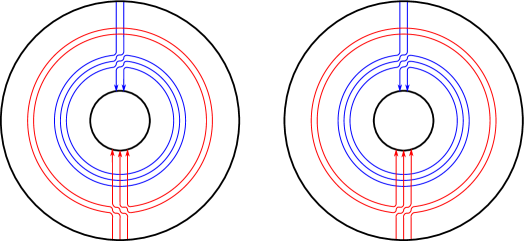
Figure 3. The configurations $\bm{\gamma}(-2,3,3,2)$ and $\bm{\gamma}(2,3,3,2)$ in $S^{1}\times I$. Note that the former is in minimal position while the latter is not.

In Construction 5.1, we have

$$\gamma_{p_{1},q_{1}}\cdot\gamma_{p_{2},q_{2}}=p_{1}q_{2}-q_{1}p_{2}\quad\text{and}\quad\left\lvert\gamma_{p_{1},q_{1}}\cap\gamma_{p_{2},q_{2}}\right\rvert=\left\lvert p_{1}q_{2}\right\rvert+\left\lvert q_{1}p_{2}\right\rvert.$$

In particular, the pair $(\gamma_{p_{1},q_{1}},\gamma_{p_{2},q_{2}})$ is in minimal position except when $p_{1}q_{2}$ and $q_{1}p_{2}$ are either both positive or both negative.

The ambient isotopy class (fixing a point on each component of $\partial A$) of each multicurve $\gamma_{p_{i},q_{i}}$ depends only on $(p_{i},q_{i})$, but the full configuration $\bm{\gamma}(p_{1},q_{1},p_{2},q_{2})$ depends a priori on more than just the isotopy classes of the individual multicurves. However, the following lemma says that when the pair $(\gamma_{p_{1},q_{1}},\gamma_{p_{2},q_{2}})$ is in minimal position, the configuration is uniquely characterized up to homeomorphism.

Lemma 5.2.

Let $r_{1},\dots,r_{k},s_{1},\dots,s_{l}$ be points in $S^{1}$, ordered cyclically according to the standard orientation of $S^{1}$. Suppose that we are given properly embedded, oriented multicurves $\alpha=\alpha_{1}\cup\dots\cup\alpha_{k}$ and $\beta=\beta_{1}\cup\dots\cup\beta_{l}$ in $A$ satisfying the following properties:

• For some fixed $[a]\in\mathbb{Z}/k$, for each $i\in\{1,\dots,k\}$, $\alpha_{i}$ is a path from $(r_{i},0)$ to $(r_{i+a},1)$ (indices modulo $k$), and any two paths $\alpha_{i},\alpha_{i^{\prime}}$ are disjoint.

• For some fixed $[b]\in\mathbb{Z}/l$, for each $j\in\{1,\dots,l\}$, $\beta_{j}$ is a path from $(s_{j},0)$ to $(s_{j+b},1)$ (indices modulo $l$), and any two paths $\beta_{j},\beta_{j^{\prime}}$ are disjoint.

• The multicurves $\alpha$ and $\beta$ intersect transversally and coherently.

Then for some integers $a$ and $b$ restricting to the given classes $[a]$ and $[b]$ and satisfying $\left\lvert al-bk\right\rvert=\left\lvert\alpha\cap\beta\right\rvert$, there is a homeomorphism of $A$ taking $(\alpha,\beta)$ to $\bm{\gamma}(a,k,b,l)$.

Proof.

For concreteness, assume that the intersection points in $\alpha_{i}\cap\beta_{j}$ all have positive sign; the other case is analogous.

Let $a$ be the representative of $[a]$ in $\{0,\dots,k-1\}$. We may identify $A$ with the quotient of the rectangle $R=[0,k]\times[0,1]$ by the relation $(0,y)\sim(k,y)$ for all $y\in[0,1]$, such that $\alpha_{i}$ is the image of $\{i\}\times[0,1]$; denote the projection map $\pi\colon\thinspace R\to A$. For $i=1,\dots,k$, note that $\pi(i,0)=(r_{i},0)$, while $\pi(i,1)=(r_{i+a},1)$ (indices modulo $k$). Therefore, $\beta$ is the image of a collection of oriented arcs $\tilde{\beta}\subset R$ with endpoints on

$$\left([0,1]\times\{0\}\right)\cup\left([k-a,k-a+1]\times\{1\}\right)\cup\left(\{0,k\}\times[0,1]\right).$$

For $i=1,\dots,k$, let $R_{i}$ denote the square $[i-1,i]\times[0,1]$. Since $\alpha$ meets $\beta$ positively, any segment of $\tilde{\beta}\cap R_{i}$ (with its inherited orientation) must enter $R_{i}$ through $\{i\}\times[0,1]$ (or through $[0,1]\times\{0\}$ if $i=1$) and exit through $\{i-1\}\times[0,1]$ (or through $[a-1,a]\times\{1\}$ if $i=a$). After an ambient isotopy of $R_{i}$, we may arrange that $\tilde{\beta}\cap R_{i}$ is a union of line segments of negative slope. Next, after an ambient isotopy of $R$ that leaves the first coordinate fixed and reparametrizes the second coordinate respecting $\sim$, we may arrange that $\tilde{\beta}$ is union of oriented line segments of negative slope beginning on

$$\left([0,1]\times\{0\}\right)\cup\left(\{k\}\times[0,1]\right)$$

and ending on

$$\left([k-a,k-a+1]\times\{1\}\right)\cup\left(\{0\}\times[0,1]\right).$$

Let $m=\left\lvert\tilde{\beta}\cap(\{0\}\times[0,1])\right\rvert=\left\lvert\tilde{\beta}\cap(\{k\}\times[0,1])\right\rvert$. Let $c$ be the number of segments of $\tilde{\beta}$ that begin on $\{k\}\times[0,1]$ and end on $[k-a,k-a+1]\times\{1\}$. After another ambient isotopy of $R$ that leaves the first coordinate fixed and reparametrizes the second coordinate respecting $\sim$, we may arrange that $\tilde{\beta}$ is a union of line segments of negative slope as above, with the additional properties that:

• $m-c$ segments end on $\{0\}\times[0,\frac{1}{2}]$, and $c$ segments end on $\{0\}\times[\frac{1}{2},1]$;

• $m-c$ segments begin on $\{k\}\times[0,\frac{1}{2}]$, and $c$ segments end on $\{k\}\times[\frac{1}{2},1]$; and

• $\tilde{\beta}\cap([0,k]\times\{\frac{1}{2}\})$ consists of $l$ points, all in the interior of $R_{1}$.

We may now reparametrize $R/{\sim}$ by the transformation

$$f(x,y)=\begin{cases}(x,y)&y\leq\frac{1}{2}\\ (x+2ay-a,y)&y\geq\frac{1}{2}.\end{cases}$$

After this reparametrization, $\beta\cap([0,k]\times[\frac{1}{2},1])/{\sim}$ can be arranged to be vertical, while $\beta\cap([0,k]\times[\frac{1}{2},1])/{\sim}$ winds with positive slope. From here, it is not hard to identify $(\alpha,\beta)$ with $\bm{\gamma}(a,k,c-m,l)$. ∎

Construction 5.3.

Returning to the notation in Construction 5.1, suppose that $\gcd(p_{1},q_{1})=\gcd(p_{2},q_{2})=1$. Decompose $S^{1}$ as a union of two arcs $e_{1}\cup e_{2}$ so that $\partial\gamma_{p_{i},q_{i}}\subset e_{i}\times\{0,1\}$. Let $R_{1}$ and $R_{2}$ be $1$-handles (i.e., copies of $I\times I$), and let $N$ be the oriented surface obtained by attaching $R_{1}$ and $R_{2}$ to $A$ along $e_{1}\times\{0,1\}$ and $e_{2}\times\{0,1\}$, respectively. For $i=1,2$, by attaching $q_{i}$ parallel cores of $R_{i}$ to $\gamma_{p_{i},q_{i}}$, we obtain a closed curve $\eta_{p_{i}/q_{i}}$. We may canonically orient these curves by requiring $q_{1},q_{2}\geq 0$ and taking the induced orientation.

5.2. Conventions for rational tangles

We briefly review some basic facts and conventions about rational tangles and their branched double covers; for further information, see [GordonPCMI, Section 4] and [Cromwell:book, Chapter 8]).

Consider the sphere $S^{2}=\partial B^{3}$, and fix an equatorial $S^{1}\subset S^{2}$. Let $Q=\{NE,NW,SW,SE\}$ be a set of four points on this $S^{1}$, ordered cyclically. By a slight abuse of notation, we shall denote by $\mu$ either the (unoriented) arc of $S^{1}$ joining $SW$ and $NW$ or the arc joining $SE$ and $NE$, and denote by $\lambda$ either the arc joining $NW$ and $NE$ or the arc joining $SW$ and $SE$. For $p/q\in\mathbb{Q}\cup\{1/0\}$, let $R(p/q)$ denote the $p/q$ rational tangle in $B^{3}$, with endpoints on $Q$; our convention is that the components of $R(1/0)$ (resp. $R(0/1)$) are pushoffs of the two choices of $\mu$ (resp. $\lambda$). Note that $R(p/q)$ can be represented with an alternating diagram such that the first crossing encountered when entering from $SW$ or $NE$ is an undercrossing, and the first crossing encountered when entering from $NW$ or $SE$ is an overcrossing, precisely when $p/q\geq 0$.

The branched double cover $\Sigma(S^{2},Q)$ is a torus, and $\Sigma(B^{3},R(p/q))$ is a solid torus. Let $\tilde{\mu}$ (resp. $\tilde{\lambda}$) be the preimage of $\mu$ (resp. $\lambda$), which up to isotopy does not depend on the choice above. We orient $\tilde{\mu}$ and $\tilde{\lambda}$ such that $\tilde{\mu}\cdot\tilde{\lambda}=-1$ when $\Sigma(S^{2},Q)$ is oriented as the boundary of $\Sigma(B^{3},R(p/q))$. As explained in [GordonPCMI, Section 4], for any $p/q\in\mathbb{Q}\cup\{1/0\}$, the curve $p\tilde{\mu}+q\tilde{\lambda}$ bounds a compressing disk in $\Sigma(B^{3},R(p/q))$.

5.3. A construction of genus-2 Heegaard diagrams

As before, for $a_{1},a_{2},a_{3},a_{4}\in\mathbb{Q}\cup\{1/0\}$, let $L(a_{1},a_{2},a_{3},a_{4})$ denote the link given by the diagram in Figure 1, where the four balls are filled in with rational tangles following the conventions described above. If $a_{1},a_{2},a_{3},a_{4}$ have the same sign, then the diagram obtained in this manner (using alternating diagrams for the rational tangles) is alternating. We now describe a construction of a Heegaard diagram for $\Sigma(L(a_{1},a_{2},a_{3},a_{4}))$.

Construction 5.4.

For $a_{i}=p_{i}/q_{i}\in{\mathbb{Q}}\cup\{1/0\}$, $i=1,\dots,4$, let $H(a_{1},a_{2},a_{3},a_{4})$ denote the Heegaard diagram shown in Figure 4. Formally, we take two copies of the configuration from Construction 5.3, denoted $(N,\eta_{-q_{1}/p_{1}},\eta_{q_{2}/p_{2}})$ and $(N^{\prime},\eta_{p_{3}/q_{3}},\eta_{-p_{4}/q_{4}})$, and form the union $S=(N\cup N^{\prime})/{\sim}$, where $R_{1}\subset N$ is identified with $R_{2}\subset N^{\prime}$, and $R_{2}\subset N$ is identified with $R_{1}\subset N^{\prime}$, each via a $90^{\circ}$ rotation of $I\times I$; we define

$$\alpha_{1} =\eta_{-q_{1}/p_{1}}\subset N \beta_{1} =\eta_{q_{2}/p_{2}}\subset N$$

$$\alpha_{2} =\eta_{p_{3}/q_{3}}\subset N^{\prime} \beta_{2} =\eta_{-p_{4}/q_{4}}\subset N^{\prime}.$$

$\alpha_{1}$ [tr] at 90 12 $\alpha_{2}$ [bl] at 258 174 $\beta_{1}$ [br] at 90 174 $\beta_{2}$ [tl] at 258 12 $p_{1}$ [tl] at 239 62 $q_{1}$ [tl] at 203 40 $p_{2}$ [br] at 20 124 $q_{2}$ [br] at 60 150 $p_{3}$ [bl] at 288 150 $q_{3}$ [bl] at 328 124 $p_{4}$ [tr] at 145 40 $q_{4}$ [tr] at 109 62

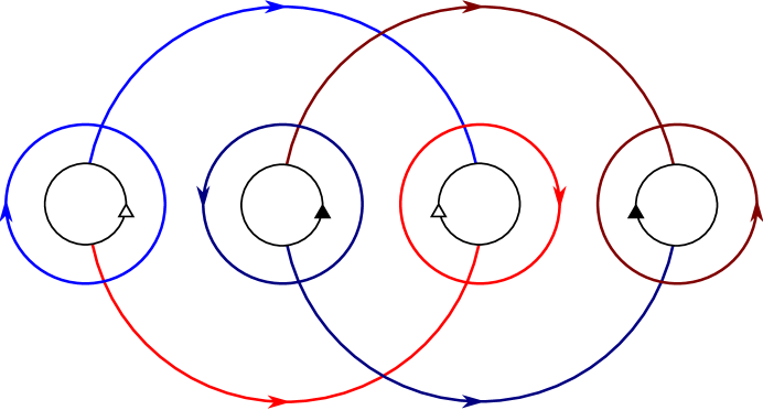
Figure 4. Template for the Heegaard diagram $H(a_{1},a_{2},a_{3},a_{4})$, $a_{i}=p_{i}/q_{i}\in{\mathbb{Q}}\cup\{1/0\}$, $i=1,\dots,4$.

Observe that

$$M(H(a_{1},a_{2},a_{3},a_{4}))=\begin{pmatrix}-p_{1}q_{2}-q_{1}p_{2}&-q_{1}p_{4}\\ -q_{2}p_{3}&p_{3}q_{4}+q_{3}p_{4}\end{pmatrix},$$

so

$$\det M(a_{1},a_{2},a_{3},a_{4})=-p_{1}q_{2}q_{3}p_{4}-q_{1}p_{2}q_{3}p_{4}-q_{1}q_{2}p_{3}p_{4},$$

while

$$\left\lvert\SS(H(a_{1},a_{2},a_{3},a_{4}))\right\rvert=\left\lvert p_{1}q_{2}q_{3}p_{4}\right\rvert+\left\lvert q_{1}p_{2}q_{3}p_{4}\right\rvert+\left\lvert q_{1}q_{2}p_{3}p_{4}\right\rvert.$$

It is easy to see that $H(a_{1},a_{2},a_{3},a_{4})$ is strong if and only if $a_{1},a_{2},a_{3},a_{4}$ all have the same sign. Additionally, note that when $a_{1}=1/0$ and $a_{3}=0/1$ or when $a_{2}=1/0$ and $a_{4}=0/1$, $H(a_{1},a_{2},a_{3},a_{4})$ is a connected sum of genus-$1$ strong diagrams.

Proposition 5.5.

For $a_{1},a_{2},a_{3},a_{4}\in{\mathbb{Q}}\cup\{1/0\}$, the Heegaard diagram $H(a_{1},a_{2},a_{3},a_{4})$ presents the manifold $\Sigma(L(a_{1},a_{2},a_{3},a_{4}))$.

Proof.

Figure 5 depicts the link $L=L(a_{1},a_{2},a_{3},a_{4})$ along with some additional decoration that we will use in order to produce a Heegaard decomposition of $\Sigma(L)$. We will then show that $H(a_{1},a_{2},a_{3},a_{4})$ presents this decomposition. The red curve $C$ in the projection plane is the cross-section of a sphere $P$ that meets $L$ in six points $x_{1},\dots,x_{6}$. The regions cut out by $C$ in the projection plane are the cross-sections of the balls cut out by $P$ in $S^{3}$. The two additional arcs in blue and yellow are cross-sections of equatorial disks $D_{1}$ and $D_{2}$ for these balls. The space $S^{3}\smallsetminus(P\cup D_{1}\cup D_{2})$ consists of four open balls whose closures we denote by $A_{1},\dots,A_{4}$; note that $(A_{i},A_{i}\cap L)$ is the rational tangle $(B^{3},R(a_{i}))$. Orient $P$ as the boundary of $A_{1}\cup A_{3}$. The double cover $V_{i}=\Sigma(A_{i},A_{i}\cap L)$ is then a solid torus, and $\Sigma(L)=V_{1}\cup\dots\cup V_{4}$.

Since $A_{1}\cap A_{3}=D_{1}$, $A_{2}\cap A_{4}=D_{2}$, and $D_{1}$ and $D_{2}$ each meet $L$ in a single point, it follows that $U_{1}=\Sigma(A_{1}\cup A_{3},(A_{1}\cup A_{3})\cap L)$ and $U_{2}=\Sigma(A_{2}\cup A_{4},(A_{2}\cup A_{4})\cap L)$ are each genus-$2$ handlebodies. Specifically, $U_{1}=V_{1}\mathbin{\natural}V_{3}$ and $U_{2}=V_{2}\mathbin{\natural}V_{4}$, where $\mathbin{\natural}$ denotes the boundary connected sum. Thus, $U_{1}\cup_{S}U_{2}$ is a genus two Heegaard decomposition of $\Sigma(L)$, where $S={\partial}U_{1}=-{\partial}U_{2}=\Sigma(P,P\cap L)$.

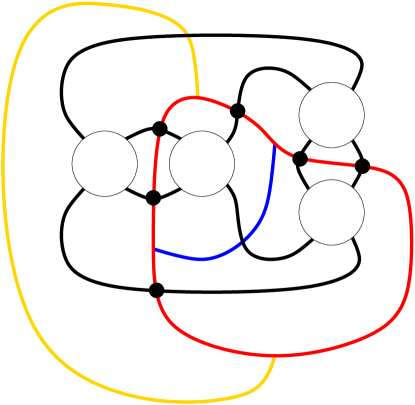
Figure 5. Decomposing $(S^{3},L(a_{1},a_{2},a_{3},a_{4}))$.

For $i=1,\dots,6$, let $C_{i}$ denote the arc of $C$ that runs clockwise from $x_{i}$ to $x_{i+1}$ in Figure 5 (subscripts mod $6$). Let $N_{i}\subset P$ denote a small regular neighborhood of $C_{i}$ and $N=N_{1}\cup\cdots\cup N_{6}$. Let $\tilde{x}_{i}$, $\gamma_{i}$, and $\gamma$ denote the respective preimages of $x_{i}$, $C_{i}$, and $C$ in $S\subset\Sigma(L)$, $i=1,\dots,6$. Then $\tilde{N}_{i}=\Sigma(N_{i},\{x_{i},x_{i+1}\})$ is an annulus with core $\gamma_{i}$, and the union $\tilde{N}=\Sigma(N,\{x_{1},\dots,x_{6}\})$ is a cyclic plumbing of these annuli. We may orient the curves $\gamma_{i}$ such that $\gamma_{i}\cdot\gamma_{i+1}=1$ for $i=1,\dots,6$. Now $S=\Sigma(P,\{x_{1},\dots,x_{6}\})$ results from gluing $A$ to the double cover of $P\smallsetminus N$, which consists of four disks; it follows that $\gamma\subset S$ appears as shown in Figure 6.

$\bullet$ at 46 128 $\bullet$ at 46 57 $\bullet$ at 175 171 $\bullet$ at 175 14 $\bullet$ at 302 128 $\bullet$ at 302 57 $\tilde{x}_{1}$ at 43 49 $\tilde{x}_{2}$ at 42 137 $\tilde{x}_{3}$ at 175 181 $\tilde{x}_{4}$ at 306 137 $\tilde{x}_{5}$ at 306 49 $\tilde{x}_{6}$ at 175 5 $\gamma_{1}$ [r] at 3 93 $\gamma_{2}$ [br] at 90 174 $\gamma_{3}$ [bl] at 258 174 $\gamma_{4}$ [l] at 345 93 $\gamma_{5}$ [tl] at 258 12 $\gamma_{6}$ [tr] at 90 12 $\gamma_{1}^{\prime}$ [tl] at 239 62 $\gamma_{4}^{\prime}$ [tr] at 109 62

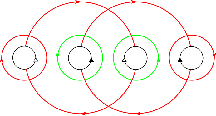
Figure 6. The surface $S=\Sigma(P,\{x_{1},\dots,x_{6}\})$ along with the branch points $\tilde{x}_{1},\dots,\tilde{x}_{6}$, the 1-complex $\gamma$ in red, and the curves $\gamma_{1}^{\prime}$, $\gamma_{4}^{\prime}$ in green. The curve $\gamma_{i}$ consists of the pair of arcs of $\gamma$ with endpoints $\tilde{x}_{i}$ and $\tilde{x}_{i+1}$. The curves $\gamma_{1}^{\prime}$ and $\gamma_{4}^{\prime}$ are parallel copies of $\gamma_{1}$ and $\gamma_{4}$, respectively.