Optimal-order preconditioners for linear systems arising in the semismooth Newton solution of a class of control-constrained problems

Abstract

In this article we present a new multigrid preconditioner for the linear systems arising in the semismooth Newton method solution of certain control-constrained, quadratic distributed optimal control problems. Using a piecewise constant discretization of the control space, each semismooth Newton iteration essentially requires inverting a principal submatrix of the matrix entering the normal equations of the associated unconstrained optimal control problem, the rows (and columns) of the submatrix representing the constraints deemed inactive at the current iteration. Previously developed multigrid preconditioners for the aforementioned submatrices were based on constructing a sequence of conforming coarser spaces, and proved to be of suboptimal quality for the class of problems considered. Instead, the multigrid preconditioner introduced in this work uses non-conforming coarse spaces, and it is shown that, under reasonable geometric assumptions on the constraints that are deemed inactive, the preconditioner approximates the inverse of the desired submatrix to optimal order. The preconditioner is tested numerically on a classical elliptic-constrained optimal control problem and further on a constrained image-deblurring problem.

1 Introduction

The goal of this work is to construct optimal order multigrid preconditioners for optimal control problems of the type

$$\min_{u\in{\mathcal{U}}}\frac{1}{2}|\!|{\mathcal{K}}u-y_{d}|\!|^{2}+\frac{\beta}{2}|\!|u|\!|^{2}\ ,\ \ a\leqslant u\leqslant b,\ \ a.e.,$$ (1)

where ${\mathcal{U}}\stackrel{{\scriptstyle\mathrm{def}}}{{=}}L^{2}(\Omega)$ with $\Omega\subset\mathbb{R}^{n}$ a bounded domain, $y_{d}\in{\mathcal{U}}$ is given, and ${\mathcal{K}}:{\mathcal{U}}\to{\mathcal{V}}$ is a linear continuous operator with ${\mathcal{V}}\hookrightarrow{\mathcal{U}}$ being a compactly embedded subspace of ${\mathcal{U}}$. The parameter $\beta>0$ is used to adjust the size of the regularization term $|\!|u|\!|^{2}$. Throughout this article $|\!|\cdot|\!|$ denotes the ${\mathcal{U}}$-norm or the operator-norm of a bounded linear operator in $\mathfrak{L}({\mathcal{U}})$. The functions $a,b\in{\mathcal{U}}$ defining the inequality constraints in (1) satisfy $a(x)<b(x)$ for all $x\in\Omega$. These problems arise in the optimal control of partial differential equations (PDEs), case in which ${\mathcal{K}}$ represents the solution operator of a PDE. For example, the classical PDE-constrained optimization problem

$$\left\{\begin{array}[]{l}\vspace{5pt}\min\ \ \frac{1}{2}|\!|y-y_{d}|\!|^{2}+\frac{\beta}{2}|\!|u|\!|^{2}\\ \vspace{5pt}\mathrm{subject\ to:}\ -\Delta y=u\ \ \mathrm{in}\ \Omega,\ \ y=0\ \ \mathrm{on}\ \partial\Omega,\\ \hskip 56.9055pta\leqslant u\leqslant b\ \ a.e.,\end{array}\right.$$ (5)

reduces to (1) when replacing $y={\mathcal{K}}u$ in the cost functional of (5), where ${\mathcal{K}}=(-\Delta)^{-1}:{\mathcal{U}}\to{\mathcal{V}}=H^{1}_{0}(\Omega)$. A related problem, discussed in [8], addresses the question of time-reversal for parabolic equations, a problem that is ill-posed. In this example we set ${\mathcal{K}}u={\mathcal{S}}(T)u$, where $t\mapsto{\mathcal{S}}(t)u$ is the time-$t$ solution operator of a linear parabolic PDE with initial value $u$, and $T>0$ is a fixed time. If the solution $u_{\min}$ of the inverse problem needs to satisfy certain inequality constraints, e.g., when $u_{\min}$, perhaps representing the concentration of a substance, is required to have values in $[0,1]$, then it is essential to impose these constraints explicitly in the formulation of the optimization problem, as shown in (1). For obvious reasons, in the PDE-constrained optimization literature (1) is referred to as the reduced problem. For other applications, such as image deblurring, ${\mathcal{K}}$ can be an explicitly defined integral operator

$${\mathcal{K}}u\stackrel{{\scriptstyle\mathrm{def}}}{{=}}\int_{\Omega}k(\cdot,x)u(x)dx\ ,$$

with $k\in{\mathcal{U}}\otimes{\mathcal{U}}$; here $u$ is the original image and $y={\mathcal{K}}u$ is the blurred image. Thus, by solving (1) we seek to reconstruct the image $u$ whose blurred version is a given $y_{d}$, subject to additional box constraints.

We give a few references to works on multigrid methods for solving (1) with no inequality constraints. In this case (1) is equivalent to the Tikhonov regularization of the ill-posed problem ${\mathcal{K}}u=y_{d}$, which in turn reduces to the linear system

$$({\mathcal{K}}^{*}{\mathcal{K}}+\beta I)u={\mathcal{K}}^{*}y_{d},$$ (6)

representing the regularized normal equations of ${\mathcal{K}}u=y_{d}$. A significant literature [17, 20, 11, 16, 8, 2, 9], to mention just a few references, is devoted to multigrid methods for (6) or the unregularized ill-posed problem. Moreover, when ${\mathcal{K}}$ is the solution operator of a linear PDE, an alternative strategy is to solve directly the indefinite systems representing the Karush-Kuhn-Tucker (KKT) optimality conditions instead of the reduced system, and many works [3, 18, 22, 23, 24] are concerned with multigrid methods for PDE-constrained optimization problems in unreduced form. A comprehensive discussion of the latter strategy is found in [4].

The presence of bound-constraints in (1) brings additional challenges to the solution process, since the KKT optimality conditions form a complementarity system as opposed to a linear or a smooth nonlinear system. As shown by Hintermüller et al. [13], the KKT system can be reformulated as a semismooth nonlinear system for which a superlinearly convergent Newton’s method can be devised – the semismooth Newton method (SSNM). Moreover, with controls discretized using piecewise constant finite elements, Hintermüller and Ulbrich [14] have shown that the SSNM converges in a mesh-independent number of iterations for problems like (1), so it is a very efficient solution method in terms of number of optimization iterations. A comprehensive discussion of SSNMs can be found in [25]. However, as with Newton’s method, each SSNM iteration requires the solution of a linear system, and the efficiency of the SSNM depends on the availability of high quality preconditioners for the linear systems involved. Naturally, the question of devising preconditioners for SSNMs has received a lot of attention in recent years, especially in the context of optimal control problems constrained by PDEs, e.g, see [12, 1, 19], where preconditioners are primarily targeting the sparse and indefinite KKT systems arising in the solution process. For problems formulated as (1), the SSNM solution essentially requires inverting at each iteration a principal submatrix of the matrix representing a discrete version ${\mathcal{H}}_{h}$ of ${\mathcal{H}}=({\mathcal{K}}^{*}{\mathcal{K}}+\beta I)$, where $h$ denotes the mesh size. The multigrid preconditioner developed by Drăgănescu and Dupont in [8] for the operator ${\mathcal{H}}_{h}$ arising in the unconstrained problem (6) is shown, under reasonable conditions, to be of optimal order with respect to the discretization: namely, if we denote by ${\mathcal{S}}_{h}$ the multigrid preconditioner (thought of as an approximation of $({\mathcal{H}}_{h})^{-1}$), then

$$1-C\frac{h^{p}}{\beta}\leqslant\frac{\left<{\mathcal{S}}_{h}u,u\right>}{\left<({\mathcal{H}}_{h})^{-1}u,u\right>}\leqslant 1+C\frac{h^{p}}{\beta},\ \ \forall u\in{\mathcal{U}}_{h}\setminus\{0\},$$ (7)

where $p>0$ is the convergence order of the discretization and ${\mathcal{U}}_{h}\subset{\mathcal{U}}$ is the discrete control space; for continuous piecewise linear discretizations we have $p=2$. A natural extension of the ideas in [8] led to the suboptimal multigrid preconditioner developed by Drăgănescu in [7] for principal submatrices of ${\mathcal{H}}_{h}$, where $p$ is shown to essentially be $1/2$ for a piecewise linear discretization. The key aspect of defining the multigrid preconditioners for principal submatrices of ${\mathcal{H}}_{h}$ is the definition of the coarse spaces. The natural domain of a principal submatrix of ${\mathcal{H}}_{h}$, thought as an operator, is a subspace of ${\mathcal{U}}_{h}$. The multigrid preconditioner developed in [7] is based on constructing coarse spaces that are subspaces of ${\mathcal{U}}_{h}$, i.e., conforming coarse spaces. A similar strategy was used by Hoppe and Kornhuber [15] in devising multilevel methods for obstacle problems. However, a visual inspection of the eigenvectors corresponding to the extreme joint eigenvalues of $({\mathcal{H}}_{h})^{-1}$ and ${\mathcal{S}}_{h}$ in [7] suggests that the multigrid preconditioner is suboptimal precisely because of the conformity of the coarse spaces. Thus in this work we defined a new multigrid preconditioner based on non-conforming coarse spaces. While the new construction is limited to piecewise constant approximations of the controls, we can show that, under reasonable conditions, the approximation order of the preconditioner in (7) is $p=1$. It also turns out that the analysis of the new preconditioner is quite different from the analysis in [7]; fortunately it is also simpler.

This article is organized as follows: in Section 2 we give a formal description of the problem and we briefly describe the SSNM to justify the necessity of preconditioning principal submatrices of ${\mathcal{H}}_{h}$. Section 3 forms the core of the article; here we introduce and analyze the two-grid preconditioner, the main result being Theorem 4. In Section 4 we extend the two-grid results to multigrid; this section follows closely the analogue extension in [7] with certain modifications required by the non-conforming coarse spaces. In Section 5 we show numerical experiments conducted on two test problems: the elliptic constrained problem (5) and the box-constrained image deblurring problem. We formulate a set of conclusions in Section 6. We included in Appendix A a convergence analysis of a Gaussian blurring operator that may also be of independent interest.

2 Problem formulation

To fix ideas we assume the compactly embedded space to be ${\mathcal{V}}\stackrel{{\scriptstyle\mathrm{def}}}{{=}}H_{0}^{1}(\Omega)$ and $\Omega$ to be polygonal or polyhedral. We denote by $|\!|u|\!|_{1}=|\!|u|\!|_{H^{1}_{0}(\Omega)}$ and we use the convention $|\!|u|\!|_{0}=|\!|u|\!|$. We also define the $H^{-1}$-norm by

$$|\!|u|\!|_{-1}\stackrel{{\scriptstyle\mathrm{def}}}{{=}}\sup_{v\in{\mathcal{V}}\setminus\{0\}}\frac{\lvert\left<u,v\right>\rvert}{|\!|v|\!|_{1}}\ ,$$

where $\left<u,v\right>$ denotes the $L^{2}(\Omega)$-inner product. We focus on a discrete version of (1) obtained by discretizing the continuous operator ${\mathcal{K}}$ using piecewise constant finite elements, as considered by Hintermüller and Ulbrich in [14]. Let $({\mathcal{T}}_{j})_{j\in\mathbb{N}}$ be a family of shape-regular, nested triangulations of $\Omega$ with with $h_{j}=\max_{T\in{\mathcal{T}}_{j}}\mathrm{diam}(T)$ being the mesh-size of the triangulation ${\mathcal{T}}_{j}$, and assume that

$$f_{low}\leqslant h_{j+1}/h_{j}\leqslant f_{high}$$ (8)

for some $0<f_{low}\leqslant f_{high}<1$ independent of $j$; for example, if $n=2$ a uniform mesh refinement leads to $f_{low}=f_{high}=1/2$. Furthermore, let ${\mathcal{U}}_{j}$ be the space of continuous piecewise constant functions with respect to ${\mathcal{T}}_{j}$. Since the triangulations are nested, we have ${\mathcal{U}}_{j}\subset{\mathcal{U}}_{j+1}$ for all $j\in\mathbb{N}$. We assume that a family of discretizations ${\mathcal{K}}_{j}\in\mathfrak{L}({\mathcal{U}}_{j},{\mathcal{V}}_{j}),\ j\in\mathbb{N}$, is given, where ${\mathcal{V}}_{j}\subset L^{2}(\Omega)$ is a finite element space with properties specified below, and ${\mathcal{K}}_{j}$ represents a discrete version of ${\mathcal{K}}$. Note that it is not assumed that ${\mathcal{V}}_{j}$ be a subspace of ${\mathcal{V}}$. The discrete optimization problem under scrutiny is

$$\min_{u\in{\mathcal{U}}_{j}}{\mathcal{J}}^{\beta}_{j}(u)\stackrel{{\scriptstyle\mathrm{def}}}{{=}}\frac{1}{2}|\!|{\mathcal{K}}_{j}u-y^{(j)}_{d}|\!|^{2}+\frac{\beta}{2}|\!|u|\!|^{2}\ ,\ \ a^{(j)}\leqslant u\leqslant b^{(j)}\ \ a.e.,$$ (9)

where $a^{(j)},b^{(j)}\in{\mathcal{U}}_{j}$ are discrete functions representing $a,b$, and $y^{(j)}_{d}=\mathrm{Proj}_{{\mathcal{V}}_{j}}y_{d}$. As in [10], we assume that the operators ${\mathcal{K}},~{}{\mathcal{K}}_{j}$ satisfy the smoothed approximation condition (SAC) appended by $L^{2}$-$L^{\infty}$ stability of ${\mathcal{K}}_{j}$:

Condition 1 (SAC).

There exists a constant $C_{1}$ depending on $\Omega,{\mathcal{T}}_{0}$ and independent of $j$ so that

1. smoothing:

   $$\max\left(|\!|{\mathcal{K}}^{*}u|\!|_{m},|\!|{\mathcal{K}}u|\!|_{m}\right)\leqslant C_{1}\left|\!\left|u\right|\!\right|,\ \ \forall u\in L^{2}(\Omega),\ m=0,1\ ;$$ (10)

2. smoothed approximation: for $j\in\mathbb{N}$

   $$|\!|{\mathcal{K}}u-{\mathcal{K}}_{j}u|\!|\leqslant C_{1}h_{j}\left|\!\left|u\right|\!\right|,\ \ \forall u\in{\mathcal{U}}_{j};$$ (11)

3. $L^{2}$-$L^{\infty}$ stability: for $j\in\mathbb{N}$

   $$|\!|{\mathcal{K}}_{j}u|\!|_{L^{\infty}(\Omega)}\leqslant C_{1}\left|\!\left|u\right|\!\right|,\ \ \forall u\in{\mathcal{U}}_{j}.$$ (12)

Remark 2.

A simple consequence of Condition 1 is that

$$|\!|{\mathcal{K}}u|\!|\leqslant C_{1}\left|\!\left|u\right|\!\right|_{-1}\ ,\ \ \forall u\in{\mathcal{U}}\ .$$ (13)

Proof.

Indeed, we have

$$|\!|{\mathcal{K}}u|\!|^{2}=\left<u,{\mathcal{K}}^{*}{\mathcal{K}}u\right>\leqslant|\!|u|\!|_{-1}\cdot|\!|{\mathcal{K}}^{*}{\mathcal{K}}u|\!|_{1}\leqslant C_{1}|\!|u|\!|_{-1}\cdot|\!|{\mathcal{K}}u|\!|\ ,$$

and (13) follows. ∎

To describe the semismooth Newton method for the discrete optimization problem, we rewrite (9) in vector form. Let $N_{j}=\mathrm{dim}({\mathcal{U}}_{j})$ and $\varphi_{1}^{(j)},\dots,\varphi_{N_{j}}^{(j)}$ be the standard piecewise constant finite element basis in ${\mathcal{T}}_{h_{j}}$. First denote by ${\bf K}_{j}$ the matrix representing the operator ${\mathcal{K}}_{j}$, and let ${\bf M}_{j}$ be the mass matrix in ${\mathcal{U}}_{j}$, and $\widetilde{{\bf M}}_{j}$ the mass matrix in ${\mathcal{V}}_{j}$. Note that the mass matrices ${\bf M}_{j}$ are diagonal. Then (9) is equivalent to

$$\min_{{\bf u}\in\mathbb{R}^{N_{j}}}J_{j}^{\beta}({\bf u})\stackrel{{\scriptstyle\mathrm{def}}}{{=}}\frac{1}{2}\lvert{\bf K}_{j}{\bf u}-{\bf y}^{(j)}_{d}\rvert^{2}_{\widetilde{{\bf M}}_{j}}+\frac{\beta}{2}\lvert{\bf u}\rvert^{2}_{{\bf M}_{j}}\ ,\ \ {\bf a}^{(j)}\leqslant{\bf u}\leqslant{\bf b}^{(j)},$$ (14)

where ${\bf y}^{(j)}_{d}$ is the vector representing $y^{(j)}_{d}$, and $\lvert{\bf u}\rvert_{{\bf M}}\stackrel{{\scriptstyle\mathrm{def}}}{{=}}\sqrt{{\bf u}^{T}{\bf M}{\bf u}}$. To simplify the exposition we omit the sub- and superscripts $j$ for the remainder of this section, so that ${\bf K}={\bf K}_{j}$, $N=N_{j}$, ${\bf a}={\bf a}^{(j)}$, etc. Similarly to (1), the discrete optimization problem (14) has a unique solution, which satisfies the KKT system

$$\left\{\begin{array}[]{l}({\bf K}^{*}{\bf K}+\beta{\bf I}){\bf u}+{\bm{\lambda}}_{a}-{\bm{\lambda}}_{b}={\bf f}\\ {\bf a}-{\bf u}\leqslant{\bf 0},\ {{\bm{\lambda}}}_{a}\geqslant 0,\ ({\bf a}-{\bf u})\cdot{{\bm{\lambda}}}_{a}={\bf 0}\\ {\bf u}-{\bf b}\leqslant{\bf 0},\ {{\bm{\lambda}}}_{b}\geqslant 0,\ ({\bf u}-{\bf b})\cdot{{\bm{\lambda}}}_{b}={\bf 0}\ ,\\ \end{array}\right.$$ (18)

where ${\bf K}^{*}={\bf M}^{-1}{\bf K}^{T}\widetilde{{\bf M}}$ is the adjoint of ${\bf K}$ with respect to the $L^{2}$-inner product, ${\bf f}={\bf K}^{*}{\bf y}_{d}$, and ${\bm{\lambda}}_{a},{\bm{\lambda}}_{b}\in\mathbb{R}^{N}$ are the Lagrange multipliers. The inequalities ${\bf u}\leqslant{\bf v}$ and the vector-valued product ${\bf u}\cdot{\bf v}$ are to be understood componentwise. The fact that we are able to write the KKT system in the form (18) is not completely obvious, and it relies on the mass matrices ${\bf M}_{j}$ being diagonal. It is worth noting that in [10, 7], where the controls were discretized using continuous piecewise linear functions, the mass-matrices were intentionally modified (equivalently to using a quadrature for computing $L^{2}$-inner products) so that they be diagonal. Following [13] (see also [7]), the complementarity problem (18) can be written as the non-smooth nonlinear system

$$\left\{\begin{array}[]{l}({\bf K}^{*}{\bf K}+\beta{\bf I}){\bf u}-{\bm{\lambda}}={\bf f}\\ {\bm{\lambda}}-\max({\bf 0},{\bf K}^{*}{\bf K}{\bf u}-{\bf f}+\beta{\bf a})-\min({\bf 0},{\bf K}^{*}{\bf K}{\bf u}-{\bf f}+\beta{\bf b})={\bf 0}\ ,\end{array}\right.$$ (21)

where ${\bm{\lambda}}=\bm{\lambda}_{a}-\bm{\lambda}_{b}$, $\bm{\lambda}_{a}=\max(\bm{\lambda},{\bf 0}),\bm{\lambda}_{b}=-\min(\bm{\lambda},{\bf 0})$. We leave it as an exercise to verify that (18) is equivalent to (21). Given the solution $({\bf u},\bm{\lambda})$ of (18), the following sets play a role in understanding the equivalence of (18) and (21):

$${\mathcal{I}} = \{i\in\{1,\dots,N\}\ :\ {\bm{\lambda}}_{i}+\beta({\bf a}_{i}-{\bf u}_{i})<0\ \ \mathrm{and}\ \ {\bm{\lambda}}_{i}+\beta({\bf b}_{i}-{\bf u}_{i})>0\}$$

$${\mathcal{A}}^{a} = \{i\in\{1,\dots,N\}\ :\ {\bm{\lambda}}_{i}+\beta({\bf a}_{i}-{\bf u}_{i})\geqslant 0\ \ \mathrm{and}\ \ {\bm{\lambda}}_{i}+\beta({\bf b}_{i}-{\bf u}_{i})>0\}$$

$${\mathcal{A}}^{b} = \{i\in\{1,\dots,N\}\ :\ {\bm{\lambda}}_{i}+\beta({\bf a}_{i}-{\bf u}_{i})<0\ \ \mathrm{and}\ \ {\bm{\lambda}}_{i}+\beta({\bf b}_{i}-{\bf u}_{i})\leqslant 0\}\ .$$

Assume (21) holds. If $i\in{\mathcal{I}}$, the second equality in (21) implies that ${\bm{\lambda}}_{i}=0$; hence ${\bf a}_{i}<{\bf u}_{i}<{\bf b}_{i}$, so the constraint corresponding to the $i^{\mathrm{th}}$ component of ${\bf u}$ is inactive. Instead, if $i\in{\mathcal{A}}^{a}$, then ${\bf u}_{i}={\bf a}_{i}$, so the lower constraints are active; similarly, if $i\in{\mathcal{A}}^{b}$, then ${\bf u}_{i}={\bf b}_{i}$, so the upper constraints are active. So, if $({\bf u},{\bm{\lambda}})$ is the solution of (21), then ${\mathcal{I}}$ is the set of indices where the constraints are inactive, ${\mathcal{A}}^{a}$ is the set of indices where the lower constraints are active, while ${\mathcal{A}}^{b}$ is the set of indices where the upper constraints are active.

The system (21) is in fact semismooth due to the fact that the function ${\bf u}\mapsto\max({\bf u},{\bf 0})$ (from $\mathbb{R}^{N}$ to $\mathbb{R}^{N}$) is slantly differentiable [13]. Consequently, (21) can be solved efficiently using the SSNM, which is equivalent to the primal-dual active set method described below, as shown in [13]. The equivalence of the two is used to prove that the convergence is superlinear. The SSNM is an iterative process that attempts to identify the sets ${\mathcal{I}},~{}{\mathcal{A}}^{a},~{}{\mathcal{A}}^{b}$ where the inequality constraints are active/inactive. More precisely, at the $k^{\mathrm{th}}$ iteration, given sets ${\mathcal{I}}_{k},~{}{\mathcal{A}}^{a}_{k},~{}{\mathcal{A}}^{b}_{k}$ partitioning $\{1,\dots,N\}$, we solve the system

$$\left\{\begin{array}[]{l}\vspace{5pt}({\bf K}^{*}{\bf K}+\beta{\bf I}){\bf u}^{(k+1)}-{\bm{\lambda}}^{(k+1)}={\bf f}\ ,\\ \vspace{5pt}{\bf u}^{(k+1)}_{i}={\bf a}_{i},\ \ \mathrm{for}\ \ i\in{\mathcal{A}}^{a}_{k},\ \ \ {\bf u}^{(k+1)}_{i}={\bf b}_{i},\ \ \mathrm{for}\ \ i\in{\mathcal{A}}^{b}_{k}\ ,\\ \vspace{5pt}{{\bm{\lambda}}}^{(k+1)}_{i}=0,\ \ \mathrm{for}\ \ i\in{\mathcal{I}}_{k}\ .\end{array}\right.$$ (25)

The solution $({\bf u}^{(k+1)},{\bm{\lambda}}^{(k+1)})$ is then used to define the new sets

$${\mathcal{I}}_{k+1} = \{i\ :\ {\bm{\lambda}}^{(k+1)}_{i}+\beta({\bf a}_{i}-{\bf u}^{(k+1)}_{i})<0\ \ \mathrm{and}\ \ {\bm{\lambda}}^{(k+1)}_{i}+\beta({\bf b}_{i}-{\bf u}^{(k+1)}_{i})>0\}\ ,$$

$${\mathcal{A}}^{a}_{k+1} = \{i\ :\ {\bm{\lambda}}^{(k+1)}_{i}+\beta({\bf a}_{i}-{\bf u}^{(k+1)}_{i})\geqslant 0\ \ \mathrm{and}\ \ {\bm{\lambda}}^{(k+1)}_{i}+\beta({\bf b}_{i}-{\bf u}^{(k+1)}_{i})>0\}\ ,$$

$${\mathcal{A}}^{b}_{k+1} = \{i\ :\ {\bm{\lambda}}^{(k+1)}_{i}+\beta({\bf a}_{i}-{\bf u}^{(k+1)}_{i})<0\ \ \mathrm{and}\ \ {\bm{\lambda}}^{(k+1)}_{i}+\beta({\bf b}_{i}-{\bf u}^{(k+1)}_{i})\leqslant 0\}\ .$$

The key problem in (25) is to identify ${\bf u}^{(k+1)}_{i}$ for $i\in{\mathcal{I}}_{k}$. If we denote the Hessian of $J^{\beta}$ from (14) by

$${\bf H}={\bf K}^{*}{\bf K}+\beta{\bf I}$$

and partition the matrix ${\bf H}$ according to the sets ${\mathcal{I}}_{k}$ and ${\mathcal{A}}_{k}={\mathcal{A}}^{a}_{k}\cup{\mathcal{A}}^{b}_{k}$

$${\bf H}^{(k)}_{\mathrm{II}}={\bf H}({\mathcal{I}}_{k},{\mathcal{I}}_{k}),\ {\bf H}^{(k)}_{\mathrm{IA}}={\bf H}({\mathcal{I}}_{k},{\mathcal{A}}_{k}),\ {\bf H}^{(k)}_{\mathrm{AI}}={\bf H}({\mathcal{A}}_{k},{\mathcal{I}}_{k}),\ {\bf H}^{(k)}_{\mathrm{AA}}={\bf H}({\mathcal{A}}_{k},{\mathcal{A}}_{k}),\$$

(we used MATLAB notation to describe submatrices) and the vectors ${\bf u}^{(k+1)}$ and $f^{(k)}$ as

$$\ {\bf u}^{(k+1)}_{\mathrm{I}}={\bf u}({\mathcal{I}}_{k}),\ {\bf u}^{(k+1)}_{\mathrm{A}}={\bf u}({\mathcal{A}}_{k}),\ {\bf f}^{(k)}_{\mathrm{I}}={\bf f}({\mathcal{I}}_{k}),\ {\bf f}^{(k)}_{\mathrm{A}}={\bf f}({\mathcal{A}}_{k}),$$

then ${\bf u}^{(k+1)}_{\mathrm{A}}$ is given explicitly in (25), $\bm{\lambda}^{(k+1)}_{\mathrm{I}}={\bf 0}$, and ${\bf u}^{(k+1)}_{\mathrm{I}}$ satisfies

$${\bf H}^{(k)}_{\mathrm{II}}{\bf u}^{(k+1)}_{\mathrm{I}}={\bf f}^{(k)}_{\mathrm{I}}-{\bf H}^{(k)}_{\mathrm{IA}}{\bf u}^{(k+1)}_{\mathrm{A}}\ .$$ (26)

The remaining components of $\bm{\lambda}^{(k+1)}$ are given by

$$\bm{\lambda}^{(k+1)}_{\mathrm{A}}={\bf H}^{(k)}_{\mathrm{AI}}{\bf u}^{(k+1)}_{\mathrm{I}}+{\bf H}^{(k)}_{\mathrm{AA}}{\bf u}^{(k+1)}_{\mathrm{A}}-{\bf f}^{(k)}_{\mathrm{A}}\ .$$

Therefore, the main challenge in solving (25) (which is a linear system) is in fact solving (26). The goal of this work is to construct and analyze multigrid preconditioners for the matrices ${\bf H}^{(k)}_{\mathrm{II}}$ appearing in (26).

3 The two-grid preconditioner

As in [10, 7], we start by designing a two-grid preconditioner for the principal submatrices of the Hessian ${\bf H}_{j}=({\bf K}_{j}^{*}{\bf K}_{j}+\beta{\bf I})$ arising in the SSNM solution process of (14), then we follow the idea in [8] to extend in Section 4 the two-grid preconditioner to a multigrid preconditioner of similar asymptotic quality. In this section we assume that we are solving (14) at a fixed level $j$, and that we reached a certain iterate $k$ in the SSNM process, with a current guess at the inactive set given by ${\mathcal{I}}^{(j)}={\mathcal{I}}^{(j)}_{k}$. Since we are not changing the SSNM iteration we discard the sub- and superscripts $k$, and we refer to ${\mathcal{I}}^{(j)}_{k}$ as the “current inactive set”.

For constructing the preconditioner it is preferable to regard the matrix ${\bf H}_{j}$ as a discretization of the operator

$${\mathcal{H}}_{j}=({\mathcal{K}}_{j}^{*}{\mathcal{K}}_{j}+\beta I)\in\mathfrak{L}({\mathcal{U}}_{j})$$

representing the Hessian of ${\mathcal{J}}^{\beta}_{j}$ in (9). We first define the (current) inactive space

$${\mathcal{U}}_{j}^{\mathrm{I}}\stackrel{{\scriptstyle\mathrm{def}}}{{=}}\mathrm{span}\{\varphi^{(j)}_{i}\ :\ i\in{\mathcal{I}}^{(j)}\}\subseteq{\mathcal{U}}_{j}\ .$$

Furthermore, denote by $\pi^{\mathrm{I}}_{j}$ the $L^{2}$-projection onto ${\mathcal{U}}^{\mathrm{I}}_{j}$ and by

$$\Omega_{j}^{\mathrm{I}}=\bigcup_{i\in{\mathcal{I}}^{(j)}}\mathrm{supp}(\varphi^{(j)}_{i})\subset\Omega$$

the inactive domain. The matrix ${\bf H}^{\mathrm{I}}_{j}$ represents the operator

$${\mathcal{H}}^{\mathrm{I}}_{j}\stackrel{{\scriptstyle\mathrm{def}}}{{=}}\pi^{\mathrm{I}}_{j}({\mathcal{K}}_{j}^{*}{\mathcal{K}}_{j}+\beta I){\mathcal{E}}_{j}^{\mathrm{I}}\in\mathfrak{L}({\mathcal{U}}_{j}^{\mathrm{I}}),$$ (27)

called here the inactive Hessian, where ${\mathcal{E}}_{j}^{\mathrm{I}}:{\mathcal{U}}^{\mathrm{I}}_{j}\to{\mathcal{U}}_{j}$ is the extension operator. Thus, our goal is to construct a two-grid preconditioner for ${\mathcal{H}}^{\mathrm{I}}_{j}$.

The first step, and perhaps the most notable achievement in this work, is the construction of an appropriate coarse space: we define the coarse inactive space as the span of all coarse basis functions whose support intersect $\Omega_{j}^{\mathrm{I}}$ nontrivially, i.e.,

$${\mathcal{U}}_{j-1}^{\mathrm{I}}\stackrel{{\scriptstyle\mathrm{def}}}{{=}}\mathrm{span}\{\varphi^{(j-1)}_{i}\ :\ i\in{\mathcal{I}}^{(j-1)}\}\subseteq{\mathcal{U}}_{j-1}\ ,$$

with

$${\mathcal{I}}^{(j-1)}\stackrel{{\scriptstyle\mathrm{def}}}{{=}}\left\{i\in\{1,\dots,N_{j-1}\}\ :\ \mu(\mathrm{supp}(\varphi_{i}^{(j-1)})\cap\Omega_{j}^{\mathrm{I}})>0\right\}\ ,$$ (28)

where $\mu$ is the Lebesgue measure in $\mathbb{R}^{n}$. Similarly, we define the coarse inactive domain by

$$\Omega_{j-1}^{\mathrm{I}}=\bigcup_{i\in{\mathcal{I}}^{(j-1)}}\mathrm{supp}(\varphi^{(j-1)}_{i})\subset\Omega\ .$$ (29)

A few remarks are in order. First, since ${\mathcal{T}}_{j}$ is a refinement of ${\mathcal{T}}_{j-1}$, it follows that the set $(\mathrm{supp}(\varphi_{i}^{(j-1)})\cap\Omega_{j}^{\mathrm{I}})$ is a (possibly empty) union of ${\mathcal{T}}_{j}$-elements. Since each element making up $\Omega_{j}^{\mathrm{I}}$ lies inside one element making up $\Omega_{j-1}^{\mathrm{I}}$, we have the inclusion

$$\Omega_{j}^{\mathrm{I}}\subseteq\Omega_{j-1}^{\mathrm{I}}\ .$$ (30)

Second, we do not expect in general that ${\mathcal{U}}_{j-1}^{\mathrm{I}}\subseteq{\mathcal{U}}_{j}^{\mathrm{I}}$. However, we have

$${\mathcal{U}}_{j-1}^{\mathrm{I}}\subseteq{\mathcal{U}}_{j}^{\mathrm{I}}\ \ \ \ \mathrm{if\ and\ only\ if}\ \ \ \ \Omega_{j-1}^{\mathrm{I}}=\Omega_{j}^{\mathrm{I}}\ .$$ (31)

We also denote

$$\partial_{\mathrm{n}}\Omega_{j}^{\mathrm{I}}\stackrel{{\scriptstyle\mathrm{def}}}{{=}}\Omega_{j-1}^{\mathrm{I}}\setminus\Omega_{j}^{\mathrm{I}},$$

a set we call the numerical boundary of $\Omega_{j}^{\mathrm{I}}$ with respect to the coarse mesh. In Figures 1 and 2 we show the sets $\Omega_{j}^{\mathrm{I}}$ (dark-gray) and $\partial_{\mathrm{n}}\Omega_{j}^{\mathrm{I}}$ (light-gray) for a few cases on uniform triangular grids on $\Omega=[0,1]\times[0,1]$.

We would like to contrast the definition (28) of the coarse indices with that of Drăgănescu [7], where a coarse basis function enters the span of the coarse inactive space if $\mathrm{supp}(\varphi_{i}^{(j-1)})\subseteq\Omega_{j}^{\mathrm{I}}$; this would define a coarse inactive space that lies inside the fine inactive space ${\mathcal{U}}^{\mathrm{I}}_{j}$, and the inclusion (30) would be reversed, that is, the coarse inactive domain would be included in the fine inactive domain.

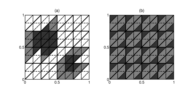
Fig. 1: In dark-gray we show $\Omega_{j}^{\mathrm{I}}$, and in light-gray we represent $\partial_{\mathrm{n}}\Omega_{j}^{\mathrm{I}}$ for $n=8$ on a uniform triangular grid. In (a) $\Omega_{j}^{\mathrm{I}}$ is the best representation of a union of two disks on the current grid; in (b) $\Omega_{j}^{\mathrm{I}}$ is a set for which $\Omega_{j-1}^{\mathrm{I}}=\Omega=[0,1]\times[0,1]$.

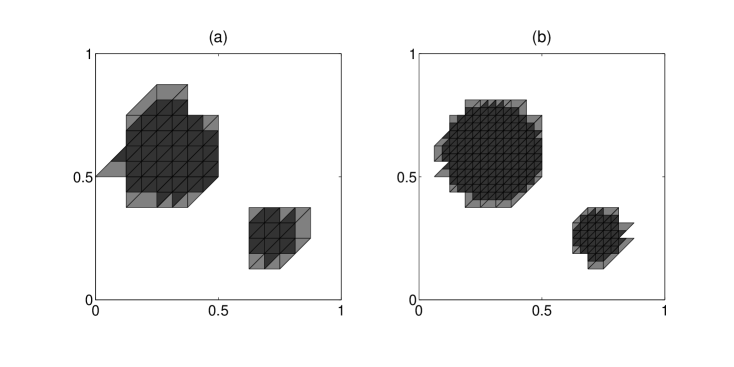
Fig. 2: In dark-gray we show $\Omega_{j}^{\mathrm{I}}$, and in light-gray we represent $\partial_{\mathrm{n}}\Omega_{j}^{\mathrm{I}}$ for $n=16$ (a) and $n=32$ (b) on a uniform triangular grid $($meshlines are omitted to enhance picture clarity$)$. For both cases, $\Omega_{j}^{\mathrm{I}}$ is the best representation on the current grid of the same union of two disks used to generate $\Omega_{j}^{\mathrm{I}}$ in Figure 1 (a). The ratio of the areas of the numerical boundaries in (b) vs. (a) is approximately $0.64$.

We now define the two-grid preconditioner ${\mathcal{M}}_{j}\in\mathfrak{L}({\mathcal{U}}_{j}^{\mathrm{I}})$ by

$${\mathcal{M}}_{j}\stackrel{{\scriptstyle\mathrm{def}}}{{=}}\pi^{\mathrm{I}}_{j}\left(({\mathcal{H}}^{\mathrm{I}}_{j-1})^{-1}\pi^{\mathrm{I}}_{j-1}+\beta^{-1}(I-\pi^{\mathrm{I}}_{j-1})\right)\ .$$ (32)

The definition (32) is rooted in the two-grid preconditioner definition from [8, 7]; the difference lies the presence of the action of the projection $\pi^{\mathrm{I}}_{j}$ as the last step in (32) (left-most term), which is necessary precisely because ${\mathcal{U}}_{j-1}^{\mathrm{I}}$ is not expected to be a subspace of ${\mathcal{U}}_{j}^{\mathrm{I}}$. An operator related to ${\mathcal{M}}_{j}$, necessary for the analysis, is

$${\mathcal{S}}_{j}\stackrel{{\scriptstyle\mathrm{def}}}{{=}}\pi^{\mathrm{I}}_{j}\left({\mathcal{H}}^{\mathrm{I}}_{j-1}\pi^{\mathrm{I}}_{j-1}+\beta(I-\pi^{\mathrm{I}}_{j-1})\right)\ .$$ (33)

Remark 3.

Both ${\mathcal{M}}_{j}$ and ${\mathcal{S}}_{j}$ are symmetric with respect to the $L^{2}$-inner product, that is,

$$\left<{\mathcal{M}}_{j}u,v\right>=\left<u,{\mathcal{M}}_{j}v\right>,\ \ \ \left<{\mathcal{S}}_{j}u,v\right>=\left<u,{\mathcal{S}}_{j}v\right>,\ \ \forall u,v\in{\mathcal{U}}_{j}^{\mathrm{I}}\ .$$

In addition, if ${\mathcal{U}}_{j-1}^{\mathrm{I}}\subseteq{\mathcal{U}}_{j}^{\mathrm{I}}$, then ${\mathcal{M}}_{j}=({\mathcal{S}}_{j})^{-1}$.

The key to the last assertions in Remark 3 is that $\pi^{\mathrm{I}}_{j}$ has no effect (hence can be discarded) when ${\mathcal{U}}_{j-1}^{\mathrm{I}}\subseteq{\mathcal{U}}_{j}^{\mathrm{I}}$. Our ultimate goal is to estimate the spectral distance between $({\mathcal{H}}^{\mathrm{I}}_{j})^{-1}$ and ${\mathcal{M}}_{j}$, as a measure of their spectral equivalence (see definition below). As an intermediate step we will estimate the spectral distance between ${\mathcal{H}}^{\mathrm{I}}_{j}$ and ${\mathcal{S}}_{j}$.

Given a Hilbert space $({\mathcal{X}},\left<\cdot,\cdot\right>)$, we denote by $\mathfrak{L}_{+}({\mathcal{X}})$ the set of symmetric positive definite operators in $\mathfrak{L}({\mathcal{X}})$. The spectral distance between $A,B\in\mathfrak{L}_{+}({\mathcal{X}})$, introduced in [8] to analyze multigrid preconditioners for inverse problems like (6), is given by

$$d_{{\mathcal{X}}}(A,B)=\sup_{u\in{\mathcal{X}}\setminus\{0\}}\left|\ln\frac{\left<Au,u\right>}{\left<Bu,u\right>}\right|\ .$$

If $\delta$ is the smallest number for which the following inequalities hold

$$1-\delta\leqslant\frac{\left<Au,u\right>}{\left<Bu,u\right>}\leqslant 1+\delta,\ \ \forall u\neq 0,$$

and $\delta\ll 1$, then $d_{{\mathcal{X}}}(A,B)\approx\delta$. The spectral distance not only allows to write the above inequalities in a more compact form, but some of its properties (including the fact that it is a distance function) are also used in the analysis. The main result in this article is the following theorem.

Theorem 4.

Assuming Condition 1 holds, there exists constants $\delta>0$ and $C_{\mathrm{tg}}>0$ independent of $j$ and the inactive set ${\mathcal{I}}^{(j)}$ so that if $\beta^{-1}(h_{j}+\mu(\partial_{\mathrm{n}}\Omega_{j}^{\mathrm{I}}))<\delta$ the following holds:

$$d_{{\mathcal{U}}_{j}^{\mathrm{I}}}({\mathcal{M}}_{j},({\mathcal{H}}^{\mathrm{I}}_{j})^{-1})\leqslant C_{\mathrm{tg}}\beta^{-1}\left(h_{j}+\mu(\partial_{\mathrm{n}}\Omega_{j}^{\mathrm{I}})\right)\ .$$ (34)

We postpone the proof of Theorem 4 after a few preliminary results.

Remark 5.

Without further formalizing the argument, we would like to comment on the optimality of the result in Theorem 4. First, it should be recognized that $\mu(\partial_{\mathrm{n}}\Omega_{j}^{\mathrm{I}})$ can be $O(1)$ for certain choices of $\Omega^{\mathrm{I}}_{j}$. For example, if ${\mathcal{T}}_{j}$ is a uniform refinement of ${\mathcal{T}}_{j-1}$ in two dimensions, and $\Omega^{\mathrm{I}}_{j}$ contains exactly one level-$j$ subdivision of each of the level-$(j-1)$ triangles that make up $\Omega$, as shown in Figure 1 $($b$)$, then ${\mathcal{U}}^{\mathrm{I}}_{j-1}={\mathcal{U}}_{j-1}$ $($the entire coarse space$)$ and $\Omega^{\mathrm{I}}_{j-1}=\Omega$; thus $\mu(\partial_{\mathrm{n}}\Omega_{j}^{\mathrm{I}})=\frac{3}{4}\mu(\Omega)$. In this case the two-grid preconditioner is not efficient. However, if $\Omega_{j}^{\mathrm{I}}$ is a good approximation of the correct inactive domain $\Omega^{\mathrm{I}}=\{x\in\Omega:a<u_{\min}(x)<b\}$, and $\Omega^{\mathrm{I}}$ is sufficiently regular, e.g., has a Lipschitz boundary, then we expect $\mu(\partial_{\mathrm{n}}\Omega_{j}^{\mathrm{I}})\approx Ch_{j}$. It is in this sense that we regard Theorem 4 as proof of the fact that the two-grid preconditioner ${\mathcal{M}}_{j}$ approximates the operator $({\mathcal{H}}^{\mathrm{I}}_{j})^{-1}$ with optimal order. Figures 1 $($b$)$ and 2 $($a$)$ and $($b$)$ show a progression of $\partial_{\mathrm{n}}\Omega_{j}^{\mathrm{I}}$ $($in gray$)$ for the case when $\Omega_{j}^{\mathrm{I}}$ is a union of two discrete representations of disks on grids with $n=8,16,32$. The ratio of the gray areas in Figure 2 $($a$)$ and $($b$)$ representing $\mu(\partial_{\mathrm{n}}\Omega_{j}^{\mathrm{I}})/\mu(\partial_{\mathrm{n}}\Omega_{j-1}^{\mathrm{I}})$ is $0.64$. Furthermore, this ratio converges to $1/2$ as the resolution tends to zero.

The optimality result in the following lemma is a critical component for the proof of Theorem 4.

Lemma 6.

There exists a constant $C_{2}$ independent of the mesh-size $h_{j}$ and the inactive set ${\mathcal{I}}^{(j)}$ so that

$$|\!|(I-\pi_{j-1}^{\mathrm{I}})u|\!|_{-1}\leqslant C_{2}h_{j}|\!|u|\!|\ ,\ \ \ \forall u\in{\mathcal{U}}_{j}^{\mathrm{I}}\ ,$$ (35)

where $(I-\pi_{j-1}^{\mathrm{I}})u$ is extended with zero outside its support.

Proof.

For $u\in{\mathcal{U}}_{j}^{\mathrm{I}}$ we have

$$|\!|(I-\pi_{j-1}^{\mathrm{I}})u|\!|_{-1} = \sup_{v\in H_{0}^{1}(\Omega)}\frac{\left<(I-\pi_{j-1}^{\mathrm{I}})u,v\right>}{|\!|v|\!|_{1}}.$$

Since $\mathrm{supp}((I-\pi_{j-1}^{\mathrm{I}})u)\subseteq\Omega_{j}^{\mathrm{I}}\cup\Omega_{j-1}^{\mathrm{I}}=\Omega_{j-1}^{\mathrm{I}}$,

$$\left<(I-\pi_{j-1}^{\mathrm{I}})u,v\right> = \left<(I-\pi_{j-1}^{\mathrm{I}})u,v-\pi_{j-1}^{\mathrm{I}}v\right>=\int_{\Omega_{j-1}^{\mathrm{I}}}((I-\pi_{j-1}^{\mathrm{I}})u)(v-\pi_{j-1}^{\mathrm{I}}v)d\mu$$

$$\leqslant |\!|(I-\pi_{j-1}^{\mathrm{I}})u|\!|_{L^{2}(\Omega_{j-1}^{\mathrm{I}})}\cdot|\!|(I-\pi_{j-1}^{\mathrm{I}})v|\!|_{L^{2}(\Omega_{j-1}^{\mathrm{I}})}$$

$$\leqslant 2|\!|u|\!|\cdot|\!|(I-\pi_{j-1}^{\mathrm{I}})v|\!|_{L^{2}(\Omega_{j-1}^{\mathrm{I}})}.$$

Now

$$|\!|(I-\pi_{j-1}^{\mathrm{I}})v|\!|^{2}_{L^{2}(\Omega_{j-1}^{\mathrm{I}})} = \sum_{i\in{\mathcal{I}}^{(j-1)}}|\!|(I-\pi_{j-1}^{\mathrm{I}})v|\!|^{2}_{L^{2}(T_{i}^{(j-1)})}$$

$$\leqslant \tilde{C}^{2}h^{2}_{j-1}\sum_{i\in{\mathcal{I}}^{(j-1)}}|v|^{2}_{H^{1}(T_{i}^{(j-1)})}\leqslant f_{low}^{-2}\tilde{C}^{2}h^{2}_{j}|v|^{2}_{H^{1}(\Omega)}\ ,$$

where $\tilde{C}$ is the constant (uniform with respect to $i$ and $j$ due to shape-regularity) appearing in the Bramble-Hilbert Lemma on each element $T_{i}^{(j-1)}$ in ${\mathcal{T}}_{j-1}$ with $i\in{\mathcal{I}}^{(j-1)}$; we also used the fact that the $L^{2}$-projection is local for the finite element space under consideration, that is, $\pi_{j-1}^{\mathrm{I}}v|_{T_{i}^{(j-1)}}$ is the average of $v$ on the element $T_{i}^{(j-1)}$. It follows that

$$\left<(I-\pi_{j-1}^{\mathrm{I}})u,v\right> \leqslant{f^{-1}_{low}}\tilde{C}h_{j}|\!|u|\!|\cdot|v|_{1},\ \ \forall v\in H_{0}^{1}(\Omega),$$

which implies the desired result with $C_{2}=f^{-1}_{low}\tilde{C}$. ∎

Remark 7.

It is remarkable that the constant $C_{2}$ is independent of the inactive set, and depends only on the constant appearing in the Bramble-Hilbert lemma and the refinement ratio. Also, what makes the optimal estimate (35) possible, is the inclusion $\Omega_{j}^{\mathrm{I}}\subseteq\Omega_{j-1}^{\mathrm{I}}$. If our choice of spaces had led to $\Omega_{j-1}^{\mathrm{I}}\not\subseteq\Omega_{j}^{\mathrm{I}}$, then the term to estimate would be $|\!|(I-\pi_{j-1}^{\mathrm{I}})v|\!|_{L^{2}(\Omega_{j}^{\mathrm{I}})}$, which is expected to be of size $\sqrt{\mu(\Omega_{j}^{\mathrm{I}}\setminus\Omega_{j-1}^{\mathrm{I}})}$; as shown in [7], the latter term is often of size $\sqrt{h_{j}}$.

Proposition 8.

Under the assumptions of Theorem 4 there exists $C_{3},\delta>0$ independent of $j,\beta$ and the fine inactive set ${\mathcal{I}}^{(j)}$ so that, if $h_{j}/\beta<\delta$, then

$$d_{{\mathcal{U}}_{j}^{\mathrm{I}}}({\mathcal{S}}_{j},{\mathcal{H}}^{\mathrm{I}}_{j})\leqslant C_{3}\frac{h_{j}}{\beta}\ .$$ (36)

Proof.

As in Lemma 6, functions are extended with zero outside their support when necessary. We have for $u\in{\mathcal{U}}_{j}^{\mathrm{I}}$

$$\left<({\mathcal{H}}^{\mathrm{I}}_{j}-{\mathcal{S}}_{j})u,u\right>$$

$$= \left<\pi^{\mathrm{I}}_{j}\left({\mathcal{K}}_{j}^{*}{\mathcal{K}}_{j}-\pi^{\mathrm{I}}_{j-1}{\mathcal{K}}_{j-1}^{*}{\mathcal{K}}_{j-1}\pi^{\mathrm{I}}_{j-1}\right)u,u\right>=\left<{\mathcal{K}}_{j}u,{\mathcal{K}}_{j}u\right>-\left<{\mathcal{K}}_{j-1}\pi^{\mathrm{I}}_{j-1}u,{\mathcal{K}}_{j-1}\pi^{\mathrm{I}}_{j-1}u\right>$$

$$= \underbrace{|\!|{\mathcal{K}}_{j}u|\!|^{2}-|\!|{\mathcal{K}}u|\!|^{2}}_{A_{1}}+\underbrace{|\!|{\mathcal{K}}u|\!|^{2}-|\!|{\mathcal{K}}\pi^{\mathrm{I}}_{j-1}u|\!|^{2}}_{A_{2}}+\underbrace{|\!|{\mathcal{K}}\pi^{\mathrm{I}}_{j-1}u|\!|^{2}-|\!|{\mathcal{K}}_{j-1}\pi^{\mathrm{I}}_{j-1}u|\!|^{2}}_{A_{3}}\ .$$

Condition 1 implies that

$$\left|A_{1}\right|=\left||\!|{\mathcal{K}}_{j}u|\!|^{2}-|\!|{\mathcal{K}}u|\!|^{2}\right| \leqslant |\!|({\mathcal{K}}_{j}-{\mathcal{K}})u|\!|\cdot\left(|\!|{\mathcal{K}}_{j}u|\!|+|\!|{\mathcal{K}}u|\!|\right)\leqslant 2C_{1}^{2}h_{j}|\!|u|\!|\ ,$$

and a similar estimate holds for the term $A_{3}$ with a constant depending on $C_{1}$ and $f_{low}$. For the second term $A_{2}$ we have

$$\left|A_{2}\right| = \left||\!|{\mathcal{K}}u|\!|^{2}-|\!|{\mathcal{K}}\pi^{\mathrm{I}}_{j-1}u|\!|^{2}\right|\leqslant|\!|{\mathcal{K}}(I-\pi^{\mathrm{I}}_{j-1})u|\!|\cdot\left(|\!|{\mathcal{K}}u|\!|+|\!|{\mathcal{K}}\pi^{\mathrm{I}}_{j-1}u|\!|\right)\$$

$$\stackrel{{\scriptstyle\eqref{eq:h1l2est},\eqref{eq:projapprox}}}{{\leqslant}} 2C_{1}^{2}C_{2}|\!|u|\!|\ .$$

The symmetry of $({\mathcal{H}}^{\mathrm{I}}_{j}-{\mathcal{S}}_{j})$ implies that

$$|\!|{\mathcal{H}}^{\mathrm{I}}_{j}-{\mathcal{S}}_{j}|\!|\leqslant C^{\prime}h_{j}\ ,$$ (37)

with $C^{\prime}$ depending on $C_{1},C_{2},f_{low}$, but not on $h_{j}$ or the inactive set ${\mathcal{I}}^{(j)}$. The rest of the argument follows closely the proof of Theorem 4.9 in [10], and we provide it for completeness. Since ${\mathcal{H}}^{\mathrm{I}}_{j}$ is symmetric and $\left<{\mathcal{H}}^{\mathrm{I}}_{j}u,u\right>\geqslant\beta|\!|u|\!|^{2},\ \forall u\in{\mathcal{U}}_{j}^{\mathrm{I}}$, it follows that

$$\sigma\left(({\mathcal{H}}^{\mathrm{I}}_{j})^{-\frac{1}{2}}\right)\subseteq(0,\beta^{-\frac{1}{2}}]\ ,\ \ \mathrm{therefore}\ \ |\!|({\mathcal{H}}^{\mathrm{I}}_{j})^{-\frac{1}{2}}|\!|\leqslant\beta^{-\frac{1}{2}}\ .$$

Hence

$$|\!|I-({\mathcal{H}}^{\mathrm{I}}_{j})^{-\frac{1}{2}}{\mathcal{S}}_{j}({\mathcal{H}}^{\mathrm{I}}_{j})^{-\frac{1}{2}}|\!|\leqslant\beta^{-1}|\!|{\mathcal{H}}^{\mathrm{I}}_{j}-{\mathcal{S}}_{j}|\!|\leqslant C^{\prime}\frac{h_{j}}{\beta}\ .$$

If $C^{\prime}h_{j}/\beta<1/2$, then

$$W\left(({\mathcal{H}}^{\mathrm{I}}_{j})^{-\frac{1}{2}}{\mathcal{S}}_{j}({\mathcal{H}}^{\mathrm{I}}_{j})^{-\frac{1}{2}}\right)=\left\{\frac{\left<{\mathcal{S}}_{j}u,u\right>}{\left<{\mathcal{H}}^{\mathrm{I}}_{j}u,u\right>}\ :\ u\in{\mathcal{U}}_{j}^{\mathrm{I}}\right\}\subseteq\left[\frac{1}{2},\frac{3}{2}\right]\ ,$$

where $W({\mathcal{A}})$ represent the numerical range of the operator ${\mathcal{A}}$. By Lemma 3.2 in [8]

$$\sup_{u\in{\mathcal{U}}_{j}^{\mathrm{I}}}\left|\ln\frac{\left<{\mathcal{S}}_{j}u,u\right>}{\left<{\mathcal{H}}^{\mathrm{I}}_{j}u,u\right>}\right|\leqslant\frac{3}{2}|\!|I-({\mathcal{H}}^{\mathrm{I}}_{j})^{-\frac{1}{2}}{\mathcal{S}}_{j}({\mathcal{H}}^{\mathrm{I}}_{j})^{-\frac{1}{2}}|\!|\leqslant\frac{3C^{\prime}}{2}\frac{h_{j}}{\beta}\ ,$$

which proves (36) with $C_{3}=3C^{\prime}/2$. ∎

Another essential element in the proof of Theorem 4 is the following additional enriched level-$j$ inactive set and associated space:

$$\widehat{{\mathcal{I}}}^{(j)} \stackrel{{\scriptstyle\mathrm{def}}}{{=}} \{i\in\{1,\dots,N_{j}\}\ :\ \mathrm{supp}(\varphi^{(j)})\subseteq\Omega_{j-1}^{\mathrm{I}}\},$$ (38)

$$\widehat{{\mathcal{U}}}_{j}^{\mathrm{I}} \stackrel{{\scriptstyle\mathrm{def}}}{{=}} \mathrm{span}\{\varphi^{(j)}\in{\mathcal{U}}_{j}\ :i\in\widehat{{\mathcal{I}}}^{(j)}\}\ .$$ (39)

It is obvious that $\widehat{{\mathcal{U}}}_{j}^{\mathrm{I}}$ includes both ${\mathcal{U}}_{j-1}^{\mathrm{I}}$ and ${{\mathcal{U}}_{j}^{\mathrm{I}}}$; it could also be regarded as the level-$j$ inactive space whose inactive domain is identical to $\Omega_{j-1}^{\mathrm{I}}$. We should also point out that the coarse inactive index set generated by $\widehat{{\mathcal{I}}}^{(j)}$ is still ${{\mathcal{I}}}^{(j-1)}$, therefore the coarse inactive space associated with $\widehat{{\mathcal{U}}}_{j}^{\mathrm{I}}$ is identical to that associated with ${{\mathcal{U}}}_{j}^{\mathrm{I}}$, namely ${\mathcal{U}}_{j-1}^{\mathrm{I}}$. Let $\widehat{\pi}_{j}^{\mathrm{I}}$ be the $L^{2}$-projection onto $\widehat{{\mathcal{U}}}_{j}^{\mathrm{I}}$ and $\widehat{{\mathcal{E}}}_{j}^{\mathrm{I}}:\widehat{{\mathcal{U}}}_{j}^{\mathrm{I}}\to{\mathcal{U}}_{j}$ be the extension operator. We now define the inactive Hessian and two-grid preconditioners associated with $\widehat{{\mathcal{I}}}^{(j)}$, all of which are to be regarded as operators in $\mathfrak{L}(\widehat{{\mathcal{U}}}_{j}^{\mathrm{I}})$:

$$\widehat{{\mathcal{H}}}^{\mathrm{I}}_{j} \stackrel{{\scriptstyle\mathrm{def}}}{{=}} \widehat{\pi}^{\mathrm{I}}_{j}({\mathcal{K}}_{j}^{*}{\mathcal{K}}_{j}+\beta I)\widehat{{\mathcal{E}}}_{j}^{\mathrm{I}},$$ (40)

$$\widehat{{\mathcal{S}}}_{j} \ \stackrel{{\scriptstyle\mathrm{def}}}{{=}}\ {\mathcal{H}}^{\mathrm{I}}_{j-1}\pi^{\mathrm{I}}_{j-1}+\beta(I-\pi^{\mathrm{I}}_{j-1}),$$ (41)

$$\widehat{{\mathcal{M}}}_{j} \ \stackrel{{\scriptstyle\mathrm{def}}}{{=}}\ ({\mathcal{H}}^{\mathrm{I}}_{j-1})^{-1}\pi^{\mathrm{I}}_{j-1}+\beta^{-1}(I-\pi^{\mathrm{I}}_{j-1}).$$ (42)

Also, let $\eta_{j}^{\mathrm{I}}:{{\mathcal{U}}}_{j}^{\mathrm{I}}\to\widehat{{\mathcal{U}}}_{j}^{\mathrm{I}}$ be the extension operator.

Lemma 9.

There exists constants $\delta>0$ and $C_{4}>0$ independent of $j$ and the inactive set $\widehat{{\mathcal{I}}}^{(j)}$ so that if $\beta^{-1}\mu(\partial_{\mathrm{n}}\Omega_{j}^{\mathrm{I}})<\delta$ then

$$d_{{\mathcal{U}}_{j}^{\mathrm{I}}}\left(({\mathcal{H}}^{\mathrm{I}}_{j})^{-1},{\pi}^{\mathrm{I}}_{j}(\widehat{{\mathcal{H}}}^{\mathrm{I}}_{j})^{-1}\eta_{j}^{\mathrm{I}}\right)\leqslant C_{4}\frac{\mu(\partial_{\mathrm{n}}\Omega_{j}^{\mathrm{I}})}{\beta}\ .$$ (43)

Proof.

The first task is to find a practical expression for the operator ${\pi}_{j}^{\mathrm{I}}(\widehat{{\mathcal{H}}}^{\mathrm{I}}_{j})^{-1}\eta_{j}^{\mathrm{I}}$. Let ${{\mathcal{U}}}^{\mathrm{I}}_{j,c}$ be the orthogonal complement of ${{\mathcal{U}}}_{j}^{\mathrm{I}}$ in $\widehat{{\mathcal{U}}}_{j}^{\mathrm{I}}$, so that $\widehat{{\mathcal{U}}}_{j}^{\mathrm{I}}={{\mathcal{U}}}_{j}^{\mathrm{I}}\oplus{{\mathcal{U}}}^{\mathrm{I}}_{j,c}$; note that functions in ${{\mathcal{U}}}^{\mathrm{I}}_{j,c}$ are supported in $\partial_{\mathrm{n}}\Omega_{j}^{\mathrm{I}}$. Furthermore, let ${\pi}^{\mathrm{I}}_{j,c}$ be the orthogonal projector on ${{\mathcal{U}}}^{\mathrm{I}}_{j,c}$ be the projector and $\eta^{\mathrm{I}}_{j,c}:{{\mathcal{U}}}^{\mathrm{I}}_{j,c}\to\widehat{{\mathcal{U}}}_{j}^{\mathrm{I}}$ be the extension operator. Following the block-splitting of the matrix representing $\widehat{{\mathcal{H}}}_{j}^{\mathrm{I}}$, we define the operators

$${\mathcal{H}}^{\mathrm{I}}_{j,oc} = \pi_{j}^{\mathrm{I}}\widehat{{\mathcal{H}}}_{j}^{\mathrm{I}}\eta^{\mathrm{I}}_{j,c}\in\mathfrak{L}({{\mathcal{U}}}^{\mathrm{I}}_{j,c},{{\mathcal{U}}}_{j}^{\mathrm{I}}),\ {\mathcal{H}}^{\mathrm{I}}_{j,co}=\pi^{\mathrm{I}}_{j,c}\widehat{{\mathcal{H}}}_{j}^{\mathrm{I}}\eta_{j}^{\mathrm{I}}\in\mathfrak{L}({{\mathcal{U}}}^{\mathrm{I}}_{j},{{\mathcal{U}}}^{\mathrm{I}}_{j,c})$$

$${\mathcal{H}}^{\mathrm{I}}_{j,cc} = \pi^{\mathrm{I}}_{j,c}\widehat{{\mathcal{H}}}_{j}^{\mathrm{I}}\eta^{\mathrm{I}}_{j,c}\in\mathfrak{L}({{\mathcal{U}}}^{\mathrm{I}}_{j,c},{{\mathcal{U}}}^{\mathrm{I}}_{j,c}).$$

Naturally, ${\mathcal{H}}_{j}^{\mathrm{I}}=\pi_{j}^{\mathrm{I}}\widehat{{\mathcal{H}}}^{\mathrm{I}}\eta_{j}^{\mathrm{I}}$, and ${{\mathcal{H}}}_{j,oc}^{\mathrm{I}}=({{\mathcal{H}}}_{j,co}^{\mathrm{I}})^{*}$. To ease notation, in the first part of this analysis we eliminate the sub- or super-scripts “$j$”, since the level does not vary, so $\widehat{{\mathcal{I}}}=\widehat{{\mathcal{I}}}^{(j)}$, $\widehat{{\mathcal{U}}}^{\mathrm{I}}=\widehat{{\mathcal{U}}}^{\mathrm{I}}_{j}$, ${{\mathcal{H}}}_{co}^{\mathrm{I}}={{\mathcal{H}}}_{j,co}^{\mathrm{I}}$, etc. Accordingly, if $\widehat{u}=u+u_{c}$ with $u\in{{\mathcal{U}}}^{\mathrm{I}},u_{c}\in{{\mathcal{U}}}^{\mathrm{I}}_{c}$, we have

$$\widehat{{\mathcal{H}}}^{\mathrm{I}}\widehat{u}=\underbrace{({{\mathcal{H}}}^{\mathrm{I}}u+{{\mathcal{H}}}_{oc}^{\mathrm{I}}u_{c})}_{\mathrm{in}\ {{\mathcal{U}}}^{\mathrm{I}}}+\underbrace{({{\mathcal{H}}}_{co}^{\mathrm{I}}u+{{\mathcal{H}}}^{\mathrm{I}}_{cc}u_{c})}_{\mathrm{in}\ {{\mathcal{U}}}^{\mathrm{I}}_{c}}\ .$$ (44)

We also define the Schur-complement of ${{\mathcal{H}}}^{\mathrm{I}}$ in $\widehat{{\mathcal{H}}}^{\mathrm{I}}$

$${\mathcal{G}}={{\mathcal{H}}}^{\mathrm{I}}_{cc}-{{\mathcal{H}}}_{co}^{\mathrm{I}}({\mathcal{H}}^{\mathrm{I}})^{-1}{{\mathcal{H}}}_{oc}^{\mathrm{I}}\ \in\mathfrak{L}({{\mathcal{U}}}^{\mathrm{I}}_{c},{{\mathcal{U}}}^{\mathrm{I}}_{c}).$$

Note that ${\mathcal{G}}$ is symmetric. For $u_{c}\in{{\mathcal{U}}}^{\mathrm{I}}_{c}$ define $u=-({\mathcal{H}}^{\mathrm{I}})^{-1}{{\mathcal{H}}}_{oc}^{\mathrm{I}}u_{c}\in{{\mathcal{U}}}^{\mathrm{I}}$ and $\widehat{u}=u+u_{c}$. A simple calculation shows that

$$\left<{\mathcal{G}}u_{c},u_{c}\right> \stackrel{{\scriptstyle\eqref{eq:hhataction}}}{{=}} \left<\widehat{{\mathcal{H}}}^{\mathrm{I}}\widehat{u},\widehat{u}\right>\geqslant\beta\left<\widehat{u},\widehat{u}\right>=\beta\left(|\!|u|\!|^{2}+|\!|u_{c}|\!|^{2}\right)\geqslant\beta|\!|u_{c}|\!|^{2}.$$ (45)

(This is simply saying that the smallest eigenvalue of the Schur-complement is greater than the smallest eigenvalue of the original operator). Hence, it follows that

$$|\!|{\mathcal{G}}^{-1}|\!|\leqslant\beta^{-1}\ .$$ (46)

When solving $\widehat{{\mathcal{H}}}^{\mathrm{I}}\widehat{u}=y$ for $y\in{{\mathcal{U}}}^{\mathrm{I}}$, standard block-elimination yields $\widehat{u}=u+u_{c}$ with

$${u}=({\mathcal{H}}^{\mathrm{I}})^{-1}\left(I+{{\mathcal{H}}}_{oc}^{\mathrm{I}}{\mathcal{G}}^{-1}{{\mathcal{H}}}_{co}^{\mathrm{I}}({\mathcal{H}}^{\mathrm{I}})^{-1}\right)y,\ \ \ u_{c}=-{\mathcal{G}}^{-1}{\mathcal{H}}_{co}^{\mathrm{I}}({\mathcal{H}}^{\mathrm{I}})^{-1}y\ .$$

The first equation above shows that

$${\pi}^{\mathrm{I}}(\widehat{{\mathcal{H}}}^{\mathrm{I}})^{-1}\eta^{\mathrm{I}}=({\mathcal{H}}^{\mathrm{I}})^{-1}\left(I+{{\mathcal{H}}}_{oc}^{\mathrm{I}}{\mathcal{G}}^{-1}{{\mathcal{H}}}_{co}^{\mathrm{I}}({\mathcal{H}}^{\mathrm{I}})^{-1}\right).$$ (47)

To estimate the spectral distance between ${\pi}^{\mathrm{I}}(\widehat{{\mathcal{H}}}^{\mathrm{I}})^{-1}\eta^{\mathrm{I}}$ and $({{\mathcal{H}}}^{\mathrm{I}})^{-1}$ we bound

$$\sup_{u\in{{\mathcal{U}}}^{\mathrm{I}}}\left|1-\frac{\left<{\pi}^{\mathrm{I}}(\widehat{{\mathcal{H}}}^{\mathrm{I}})^{-1}\eta^{\mathrm{I}}u,u\right>}{\left<({{\mathcal{H}}}^{\mathrm{I}})^{-1}u,u\right>}\right|$$ (48)

$$\stackrel{{\scriptstyle\eqref{eq:extHinv}}}{{=}} \sup_{u\in{{\mathcal{U}}}^{\mathrm{I}}\setminus\{0\}}\left|\frac{\left<({\mathcal{H}}^{\mathrm{I}})^{-1}{{\mathcal{H}}}_{oc}^{\mathrm{I}}{\mathcal{G}}^{-1}{{\mathcal{H}}}_{co}^{\mathrm{I}}({\mathcal{H}}^{\mathrm{I}})^{-1}u,u\right>}{\left<({{\mathcal{H}}}^{\mathrm{I}})^{-1}u,u\right>}\right|$$

$$\stackrel{{\scriptstyle v=({\mathcal{H}}^{\mathrm{I}})^{-\frac{1}{2}}u}}{{=}} \sup_{v\in{{\mathcal{U}}}^{\mathrm{I}}\setminus\{0\}}\left|\frac{\left<({\mathcal{H}}^{\mathrm{I}})^{-\frac{1}{2}}{{\mathcal{H}}}_{oc}^{\mathrm{I}}{\mathcal{G}}^{-1}{{\mathcal{H}}}_{co}^{\mathrm{I}}({\mathcal{H}}^{\mathrm{I}})^{-\frac{1}{2}}v,v\right>}{\left<v,v\right>}\right|=|\!|({\mathcal{H}}^{\mathrm{I}})^{-\frac{1}{2}}{{\mathcal{H}}}_{oc}^{\mathrm{I}}{\mathcal{G}}^{-1}{{\mathcal{H}}}_{co}^{\mathrm{I}}({\mathcal{H}}^{\mathrm{I}})^{-\frac{1}{2}}|\!|$$

$$\leqslant |\!|({\mathcal{H}}^{\mathrm{I}})^{-\frac{1}{2}}{{\mathcal{H}}}_{oc}^{\mathrm{I}}|\!|^{2}\cdot|\!|{\mathcal{G}}^{-1}|\!|\leqslant\beta^{-1}|\!|({\mathcal{H}}^{\mathrm{I}})^{-\frac{1}{2}}{{\mathcal{H}}}_{oc}^{\mathrm{I}}|\!|^{2}\ ,$$

since $|\!|({\mathcal{H}}^{\mathrm{I}})^{-\frac{1}{2}}{{\mathcal{H}}}_{oc}^{\mathrm{I}}|\!|=|\!|{{\mathcal{H}}}_{co}^{\mathrm{I}}({\mathcal{H}}^{\mathrm{I}})^{-\frac{1}{2}}|\!|$ as they are dual to each other.

We resume using the index $j$ as we estimate $|\!|({\mathcal{H}}_{j}^{\mathrm{I}})^{-\frac{1}{2}}{{\mathcal{H}}}_{j,oc}^{\mathrm{I}}|\!|$. Following (45), for all $u_{c}\in{{\mathcal{U}}}^{\mathrm{I}}_{j,c}$

$$|\!|({\mathcal{H}}_{j}^{\mathrm{I}})^{-\frac{1}{2}}{{\mathcal{H}}}_{j,oc}^{\mathrm{I}}u_{c}|\!|^{2} = \left<{{\mathcal{H}}}_{j,co}^{\mathrm{I}}({\mathcal{H}}_{j}^{\mathrm{I}})^{-1}{{\mathcal{H}}}_{j,oc}^{\mathrm{I}}u_{c},u_{c}\right>\stackrel{{\scriptstyle\eqref{eq:coercG}}}{{\leqslant}}\left<({{\mathcal{H}}}^{\mathrm{I}}_{j,cc}-\beta I)u_{c},u_{c}\right>$$

$$\leqslant \left<\pi^{\mathrm{I}}_{j,c}(\widehat{{\mathcal{H}}}_{j}^{\mathrm{I}}-\beta I)\eta^{\mathrm{I}}_{j,c}u_{c},u_{c}\right>.$$

If we define by ${{\mathcal{E}}}_{j,c}^{\mathrm{I}}\in\mathfrak{L}({{\mathcal{U}}}^{\mathrm{I}}_{j,c},{{\mathcal{U}}}_{j})$ the extension-with-zero operator, then

$$\pi^{\mathrm{I}}_{j,c}(\widehat{{\mathcal{H}}}_{j}^{\mathrm{I}}-\beta I)\eta^{\mathrm{I}}_{j,c}=\pi^{\mathrm{I}}_{j,c}({\mathcal{K}}_{j}^{*}{\mathcal{K}}_{j}){{\mathcal{E}}}_{j,c}^{\mathrm{I}}.$$

Therefore,

$$|\!|({\mathcal{H}}_{j}^{\mathrm{I}})^{-\frac{1}{2}}{{\mathcal{H}}}_{j,oc}^{\mathrm{I}}u_{c}|\!|^{2} \leqslant \left<\pi^{\mathrm{I}}_{j,c}({\mathcal{K}}_{j}^{*}{\mathcal{K}}_{j}){{\mathcal{E}}}_{j,c}^{\mathrm{I}}u_{c},u_{c}\right>=|\!|{\mathcal{K}}_{j}{{\mathcal{E}}}_{j,c}^{\mathrm{I}}u_{c}|\!|^{2}$$

$$\leqslant |\!|{\mathcal{K}}_{j}{{\mathcal{E}}}_{j,c}^{\mathrm{I}}u_{c}|\!|_{L^{\infty}(\partial_{\mathrm{n}}\Omega_{j}^{\mathrm{I}})}^{2}\>\mu(\partial_{\mathrm{n}}\Omega_{j}^{\mathrm{I}})$$

$$\stackrel{{\scriptstyle\eqref{cond:l2linf}}}{{\leqslant}} C_{1}^{2}|\!|{{\mathcal{E}}}_{j,c}^{\mathrm{I}}u_{c}|\!|_{L^{2}(\Omega)}^{2}\>\mu(\partial_{\mathrm{n}}\Omega_{j}^{\mathrm{I}})=C_{1}^{2}|\!|u_{c}|\!|^{2}\>\mu(\partial_{\mathrm{n}}\Omega_{j}^{\mathrm{I}})\ .$$

It follows that

$$|\!|({\mathcal{H}}_{j}^{\mathrm{I}})^{-\frac{1}{2}}{{\mathcal{H}}}_{j,oc}^{\mathrm{I}}|\!|\leqslant C_{1}\sqrt{\mu(\partial_{\mathrm{n}}\Omega_{j}^{\mathrm{I}})}\ .$$ (49)

So, by (48) and (49) we get

$$\sup_{u\in{{\mathcal{U}}}_{j}^{\mathrm{I}}}\left|1-\frac{\left<{\pi}_{j}^{\mathrm{I}}(\widehat{{\mathcal{H}}}_{j}^{\mathrm{I}})^{-1}\eta_{j}^{\mathrm{I}}u,u\right>}{\left<({{\mathcal{H}}}_{j}^{\mathrm{I}})^{-1}u,u\right>}\right|\leqslant C_{1}^{2}\beta^{-1}\mu(\partial_{\mathrm{n}}\Omega_{j}^{\mathrm{I}})\ .$$

If $C_{1}^{2}\beta^{-1}\mu(\partial_{\mathrm{n}}\Omega_{j}^{\mathrm{I}})<\frac{1}{2}$, by Lemma 3.2 in [8]

$$\left|\ln\frac{\left<{\pi}_{j}^{\mathrm{I}}(\widehat{{\mathcal{H}}}_{j}^{\mathrm{I}})^{-1}\eta_{j}^{\mathrm{I}}u,u\right>}{\left<({{\mathcal{H}}}_{j}^{\mathrm{I}})^{-1}u,u\right>}\right|\leqslant\frac{3}{2}C_{1}^{2}\beta^{-1}\mu(\partial_{\mathrm{n}}\Omega_{j}^{\mathrm{I}})\ ,$$

which concludes the proof. ∎

We now return to the proof of Theorem 4.

Proof.

We refer to the space $\widehat{{\mathcal{U}}}_{j}^{\mathrm{I}}$ defined in (39) and the associated operators $\widehat{{\mathcal{H}}}^{\mathrm{I}}_{j},\widehat{{\mathcal{S}}}_{j},\widehat{{\mathcal{M}}}_{j}$ defined in (40)-(42). Cf. Remark 3, because ${\mathcal{U}}_{j-1}^{\mathrm{I}}\subseteq\widehat{{\mathcal{U}}}_{j}^{\mathrm{I}}$, we have $(\widehat{{\mathcal{S}}}_{j})^{-1}=\widehat{{\mathcal{M}}}_{j}\ .$ By Lemma 3.10 in [8] we have

$$d_{\widehat{{\mathcal{U}}}_{j}^{\mathrm{I}}}\left(\widehat{{\mathcal{M}}}_{j},(\widehat{{\mathcal{H}}}^{\mathrm{I}}_{j})^{-1}\right)=d_{\widehat{{\mathcal{U}}}_{j}^{\mathrm{I}}}\left(\widehat{{\mathcal{S}}}_{j},\widehat{{\mathcal{H}}}^{\mathrm{I}}_{j}\right)\ .$$ (50)

Hence,

$$d_{{{\mathcal{U}}}_{j}^{\mathrm{I}}}\left({{\mathcal{M}}}_{j},({{\mathcal{H}}}^{\mathrm{I}}_{j})^{-1}\right)$$

$$= \sup_{u\in{{\mathcal{U}}}_{j}^{\mathrm{I}}\setminus\{0\}}\left|\ln\frac{\left<{\pi}^{\mathrm{I}}_{j}\left(\left({\mathcal{H}}^{\mathrm{I}}_{j-1}\right)^{-1}\pi^{\mathrm{I}}_{j-1}+\beta^{-1}(I-\pi^{\mathrm{I}}_{j-1})\right)u,u\right>}{\left<({{\mathcal{H}}}^{\mathrm{I}}_{j})^{-1}u,u\right>}\right|$$

$$\stackrel{{\scriptstyle{\mathcal{U}}_{j}^{\mathrm{I}}\subseteq\widehat{{\mathcal{U}}}_{j}^{\mathrm{I}}}}{{=}} \sup_{u\in{{\mathcal{U}}}_{j}^{\mathrm{I}}\setminus\{0\}}\left|\ln\frac{\left<\widehat{\pi}^{\mathrm{I}}_{j}\left(\left({\mathcal{H}}^{\mathrm{I}}_{j-1}\right)^{-1}\pi^{\mathrm{I}}_{j-1}+\beta^{-1}(I-\pi^{\mathrm{I}}_{j-1})\right)u,u\right>}{\left<({{\mathcal{H}}}^{\mathrm{I}}_{j})^{-1}u,u\right>}\right|$$

$$\leqslant \sup_{u\in{{\mathcal{U}}}_{j}^{\mathrm{I}}\setminus\{0\}}\left|\ln\frac{\left<\widehat{{\mathcal{M}}}_{j}u,u\right>}{\left<(\widehat{{\mathcal{H}}}^{\mathrm{I}}_{j})^{-1}u,u\right>}\right|+\sup_{u\in{{\mathcal{U}}}_{j}^{\mathrm{I}}\setminus\{0\}}\left|\ln\frac{\left<(\widehat{{\mathcal{H}}}^{\mathrm{I}}_{j})^{-1}u,u\right>}{\left<({{\mathcal{H}}}^{\mathrm{I}}_{j})^{-1}u,u\right>}\right|$$

$$\leqslant d_{\widehat{{\mathcal{U}}}_{j}^{\mathrm{I}}}\left(\widehat{{\mathcal{M}}}_{j},(\widehat{{\mathcal{H}}}^{\mathrm{I}}_{j})^{-1}\right)+\sup_{u\in{{\mathcal{U}}}_{j}^{\mathrm{I}}\setminus\{0\}}\left|\ln\frac{\left<(\widehat{{\mathcal{H}}}^{\mathrm{I}}_{j})^{-1}u,u\right>}{\left<({{\mathcal{H}}}^{\mathrm{I}}_{j})^{-1}u,u\right>}\right|$$

$$\stackrel{{\scriptstyle\eqref{eq:specdistinv}}}{{=}} d_{\widehat{{\mathcal{U}}}_{j}^{\mathrm{I}}}\left(\widehat{{\mathcal{S}}}_{j},\widehat{{\mathcal{H}}}^{\mathrm{I}}_{j}\right)+\sup_{u\in{{\mathcal{U}}}_{j}^{\mathrm{I}}\setminus\{0\}}\left|\ln\frac{\left<{\pi}^{\mathrm{I}}_{j}(\widehat{{\mathcal{H}}}^{\mathrm{I}}_{j})^{-1}u,u\right>}{\left<({{\mathcal{H}}}^{\mathrm{I}}_{j})^{-1}u,u\right>}\right|.$$

By Proposition 8, the first term above is bounded by $C_{3}\beta^{-1}h_{j}$, assuming $\beta^{-1}h_{j}$ is sufficiently small. The second term expresses the spectral distance between ${\pi}^{\mathrm{I}}_{j}(\widehat{{\mathcal{H}}}^{\mathrm{I}}_{j})^{-1}\eta_{j}^{\mathrm{I}}$ and $({{\mathcal{H}}}^{\mathrm{I}}_{j})^{-1}$, and is bounded by $C_{4}\beta^{-1}\mu(\partial_{\mathrm{n}}\Omega_{j}^{\mathrm{I}})$ provided $\beta^{-1}\mu(\partial_{\mathrm{n}}\Omega_{j}^{\mathrm{I}})$ is sufficiently small, cf. Lemma 9, which concludes the proof. ∎

4 The multigrid preconditioner

The extension of the two-grid preconditioner introduced in Section 3 to a multigrid preconditioner follows closely [7]. However, since the use of non-conforming spaces requires a few changes both in the construction and the analysis, we give here a full description of the extension process. As in [7], we adopt the following point of view: the level for which we construct a multigrid preconditioner is given to be $j$ and is considered fixed, and we also fix an inactive set ${\mathcal{I}}^{(j)}$, which corresponds to one of the SSNM iterations. This leads to the definition of ${\mathcal{H}}^{\mathrm{I}}_{j}$ as in (27). As with other multigrid methods for integral equations of the second kind, the base level, denoted by $j_{0}$, may not necessarily be the coarsest case available, i.e., $j_{0}=0$, but has to sufficiently fine for the conditions in Theorem 15 below to be satisfied. The goal is to construct the operator ${\mathcal{Z}}_{j}$ representing the multigrid preconditioner for ${\mathcal{H}}^{\mathrm{I}}_{j}$, i.e., an approximation of $({\mathcal{H}}^{\mathrm{I}}_{j})^{-1}$.

4.1 Construction and complexity

The first step in building the multigrid preconditioner is to construct the coarse inactive spaces and operators for the levels $k=j-1,j-2,\dots,j_{0}$, in accordance with (28). More precisely, after defining

$$\Omega_{j}^{\mathrm{I}}=\bigcup_{i\in{\mathcal{I}}^{(j)}}\mathrm{supp}(\varphi^{(j)}_{i}),$$

we construct recursively the coarser inactive index-sets, domains, and spaces.

Algorithm 10 (Inactive set, inactive domain definition).

1. for  $k=(j-1)\>:\>-1\>:\>j_{0}$

2. ${\mathcal{I}}^{(k)}\stackrel{{\scriptstyle\mathrm{def}}}{{=}}\left\{i\in\{1,\dots,N_{k}\}\ :\ \mu(\mathrm{supp}(\varphi_{i}^{(k)})\cap\Omega_{k+1}^{\mathrm{I}})>0\right\}$

3. $\Omega_{k}^{\mathrm{I}}\stackrel{{\scriptstyle\mathrm{def}}}{{=}}\bigcup_{i\in{\mathcal{I}}^{(k)}}\mathrm{supp}(\varphi^{(k)}_{i})$

4. end

With inactive index-sets constructed, we now define, as before, the inactive spaces and operators for $k=j_{0},\dots,j$:

$${\mathcal{U}}_{k}^{\mathrm{I}} \stackrel{{\scriptstyle\mathrm{def}}}{{=}} \mathrm{span}\{\varphi^{(k)}_{i}\ :\ i\in{\mathcal{I}}^{(k)}\}\ ,$$

$${\mathcal{H}}^{\mathrm{I}}_{k} \stackrel{{\scriptstyle\mathrm{def}}}{{=}} \pi^{\mathrm{I}}_{k}({\mathcal{K}}_{k}^{*}{\mathcal{K}}_{k}+\beta I){\mathcal{E}}_{k}^{\mathrm{I}}\in\mathfrak{L}({\mathcal{U}}_{k}^{\mathrm{I}})\ .$$

Recall that ${\mathcal{U}}_{k}^{\mathrm{I}}\subseteq{\mathcal{U}}_{k}$, but we do not expect in general that ${\mathcal{U}}_{k}^{\mathrm{I}}\subseteq{\mathcal{U}}_{k+1}^{\mathrm{I}}$. However, the inclusion $\Omega_{k+1}^{\mathrm{I}}\subseteq\Omega_{k}^{\mathrm{I}}$ holds for $k=j_{0},\dots,j-1$. We also define for $k=1,2,\dots$ the operators

$$\mathfrak{I}_{k-1}^{k}:\mathfrak{L}({\mathcal{U}}_{k-1}^{\mathrm{I}})\to\mathfrak{L}({\mathcal{U}}_{k}^{\mathrm{I}}),\ \ \mathfrak{I}_{k-1}^{k}({\mathcal{X}})=\pi_{k}^{\mathrm{I}}\left({\mathcal{X}}\cdot\pi_{k-1}^{\mathrm{I}}+\beta^{-1}(I-\pi_{k-1}^{\mathrm{I}})\right).$$ (51)

Note that the two-grid preconditioner ${\mathcal{M}}_{j}$ can be written as

$${\mathcal{M}}_{j}=\mathfrak{I}_{j-1}^{j}\left(({\mathcal{H}}^{\mathrm{I}}_{j-1})^{-1}\right)\ .$$ (52)

Another essential element in defining the multigrid preconditioner is the family of operators $\mathfrak{N}_{k}$, $k=j_{0},\dots,j$, given by

$$\mathfrak{N}_{k}:\mathfrak{L}({\mathcal{U}}_{k}^{\mathrm{I}})\to\mathfrak{L}({\mathcal{U}}_{k}^{\mathrm{I}}),\ \ \mathfrak{N}_{k}({\mathcal{X}})\stackrel{{\scriptstyle\mathrm{def}}}{{=}}2{\mathcal{X}}-{\mathcal{X}}\cdot{\mathcal{H}}_{k}^{\mathrm{I}}\cdot{\mathcal{X}}\ .$$

It is known that ${\mathcal{X}}_{l+1}=\mathfrak{N}_{k}({\mathcal{X}}_{l})$, $l=1,2,\dots$, represents the Newton iteration for solving the nonlinear operator-equation ${\mathcal{X}}^{-1}-{\mathcal{H}}_{k}^{\mathrm{I}}=0$ (e.g., see [8]).

The following algorithm produces for $k=j_{0}+1,\dots,j$ a sequence of operators ${\mathcal{Z}}_{k}\in\mathfrak{L}({\mathcal{U}}_{k}^{\mathrm{I}})$, of which ${\mathcal{Z}}_{j}$ is the desired multigrid preconditioner.

Algorithm 11 (Operator-form definition of ${\mathcal{Z}}_{k}$; input arguments: $j\geqslant j_{0}+1$).

1. ${\mathcal{Z}}_{j_{0}}\stackrel{{\scriptstyle\mathrm{def}}}{{=}}({\mathcal{H}}^{\mathrm{I}}_{j_{0}})^{-1}$                        % base level

2. for  $k=j_{0}+1:j-1$               % intermediate levels (if any)

3. ${\mathcal{Z}}_{k}\stackrel{{\scriptstyle\mathrm{def}}}{{=}}\mathfrak{N}_{k}(\mathfrak{I}_{k-1}^{k}({\mathcal{Z}}_{k-1}))$

4. end

5. ${\mathcal{Z}}_{j}\stackrel{{\scriptstyle\mathrm{def}}}{{=}}\mathfrak{I}_{j-1}^{j}({\mathcal{Z}}_{j-1})$                      % finest level

Algorithm 11 shows that ${\mathcal{Z}}_{j}$ has a W-cycle structure. Moreover, for $k<j$, applying ${\mathcal{Z}}_{k}$ involves one application of ${\mathcal{H}}_{k}^{\mathrm{I}}$. To estimate the cost of applying ${\mathcal{Z}}_{j}$ we make some assumptions with respect to the cost of applying ${\mathcal{H}}_{k}^{\mathrm{I}}$ and the cost of inverting ${\mathcal{H}}^{\mathrm{I}}_{j_{0}}$ at step 1 using unpreconditioned conjugate gradient (CG). Recall that $N_{k}=\mathrm{dim}({\mathcal{U}}_{k})$, and assume that there exists $\alpha\in(0,1)$ so that $N_{k-1}\leqslant\alpha N_{k}$, $k=1,2,\dots$; we expect $\alpha\approx 2^{-n}$, where $n$ is the dimension of the ambient space. We also assume that the cost of applying the Hessian ${\mathcal{H}}_{k}$, and hence ${\mathcal{H}}^{\mathrm{I}}_{k}$, is

$$t(k)\approx C_{op}N_{k}^{p},\ \ p\geqslant 1.$$

For the elliptic-constrained problem (5) we take $p=1$ if we use classical multigrid for solving the elliptic problems, while for the image deblurring example we have $p=2$. We assume that the cost of applying ${\mathcal{H}}_{k}$ dominates the added $O(N_{k})$-costs of projecting vectors onto the coarse space and other usual vector additions in the preconditioner, hence we discard the latter from the cost computation. The last hypothesis is that for any level $k$, CG converges to the desired tolerance in at most $F_{cg}$ iterations at a cost of $cF_{cg}N_{k}$ flops. In practice we have seen $F_{cg}$ to range between $10-100$ on a variety of problems. It follows from Algorithm 11 that the cost $f(k)$ of applying ${\mathcal{Z}}_{k}$ satisfies the recursion:

$$f(j) \leqslant f({j-1})+O(N_{j})\approx f({j-1})$$ (53)

$$f(k) \leqslant 2f({k-1})+t(k),\ \ k=j_{0}+1,\dots,j-1$$

$$f({j_{0}}) \leqslant cF_{cg}N_{j_{0}}.$$

Assuming that $2\alpha^{p}<1$, a standard argument shows that

$$f({j-1})\leqslant 2^{j-j_{0}-1}cF_{cg}N_{j_{0}}+C_{op}\frac{1-(2\alpha^{p})^{j-j_{0}-1}}{1-2\alpha^{p}}N_{j-1}^{p}.$$

If we denote by $l=j-j_{0}+1$ the number of levels used (i.e., $j=j_{0}+2$ meaning three levels) and discard the $O(N_{j})$ term in (53), then

$$f({j})\leqslant\left((2\alpha)^{l-1}F_{cg}\frac{c}{2C_{op}}+\frac{\alpha^{p}}{1-2\alpha^{p}}(1-(2\alpha^{p})^{l-2})\right)\overbrace{C_{op}N_{j}^{p}}^{t(j)}.$$ (54)

The expression above is not expected to be consistent with the cases $l=1,2$ due to the neglection of the costs of projections. Formula (54) shows that it is certainly advantageus to use as many levels as possible to keep the cost $f(j)$ of applying the preconditioner ${\mathcal{Z}}_{j}$ low relative to the cost $t(j)$ of applying the inactive Hessian ${\mathcal{H}}^{\mathrm{I}}_{j}$. Asymptotically, if $l$ is large, then

$$f(j)\approx\frac{\alpha^{p}}{(1-2\alpha^{p})}t(j)\ .$$ (55)

If $\alpha$ is truly small due to high-dimensionality and/or the cost of applying the Hessian is high (either $C_{op}\gg c$ or $p>1$), then the relative cost $f(j)/t(j)$ can be small even with a low number of levels. We expect the wall-clock timings we show in Section 5 to give a better picture of the computational savings of using the multigrid preconditioned conjugate gradient (MGCG) versus CG.

However, we must point out that our computations are only two-dimensional, so $\alpha\approx 1/2$. Thus, in order to notice significant savings in computing time, we need either high-resolution and/or many levels. For higher dimensions (three and four), the factor $\alpha^{p}$ in (55) is expected to be significantly smaller, resulting in a much lower cost of applying the multigrid preconditioner. Thus we anticipate that the wall-clock savings in higher dimensional problems will occur at lower resolutions as for two-dimensional problems.

4.2 Analysis

Estimating the spectral distance between the multigrid preconditioner ${\mathcal{Z}}_{j}$ and $({\mathcal{H}}^{\mathrm{I}}_{j})^{-1}$ follows the same path as the analysis in [7]. The only significant difference lies in the presence of the projection $\pi_{k}^{\mathrm{I}}$ in the operator $\mathfrak{I}_{k-1}^{k}$ defined in (51). We now verify that $\mathfrak{I}_{k-1}^{k}$ is non-expansive in the spectral distance, a result similar to Lemma 4.2 in  [7].

Lemma 12.

For $k=1,2,\dots$, and ${\mathcal{X}}\in\mathfrak{L}_{+}({\mathcal{U}}_{k-1}^{\mathrm{I}})$, we have $\mathfrak{I}_{k-1}^{k}({\mathcal{X}})\in\mathfrak{L}_{+}({\mathcal{U}}_{k}^{\mathrm{I}})$. Moreover, if ${\mathcal{X}},~{}{\mathcal{Y}}\in\mathfrak{L}_{+}({\mathcal{U}}_{k-1}^{\mathrm{I}})$, then

$$d_{{\mathcal{U}}_{k}^{\mathrm{I}}}(\mathfrak{I}_{k-1}^{k}({\mathcal{X}}),\mathfrak{I}_{k-1}^{k}({\mathcal{Y}}))\leqslant d_{{\mathcal{U}}_{k-1}^{\mathrm{I}}}({\mathcal{X}},{\mathcal{Y}})\ .$$ (56)

Proof. If ${\mathcal{X}}\in\mathfrak{L}_{+}({\mathcal{U}}_{k-1}^{\mathrm{I}})$, then for $u,v\in{\mathcal{U}}_{k}^{\mathrm{I}}$ we have

$$\left<\pi_{k}^{\mathrm{I}}{\mathcal{X}}\pi_{k-1}^{\mathrm{I}}u,v\right> = \left<{\mathcal{X}}\pi_{k-1}^{\mathrm{I}}u,v\right>=\left<{\mathcal{X}}\pi_{k-1}^{\mathrm{I}}u,\pi_{k-1}^{\mathrm{I}}v\right>=\left<\pi_{k-1}^{\mathrm{I}}u,{\mathcal{X}}\pi_{k-1}^{\mathrm{I}}v\right>$$

$$= \left<u,{\mathcal{X}}\pi_{k-1}^{\mathrm{I}}v\right>=\left<u,\pi_{k}^{\mathrm{I}}{\mathcal{X}}\pi_{k-1}^{\mathrm{I}}v\right>,$$

which shows that $\pi_{k}^{\mathrm{I}}{\mathcal{X}}\pi_{k-1}^{\mathrm{I}}$ is symmetric (recall that neither of ${\mathcal{U}}_{k-1}^{\mathrm{I}}$ and ${\mathcal{U}}_{k}^{\mathrm{I}}$ are assumed to be subspaces of each other). Given the symmetry of the orthogonal projection $\pi_{k}^{\mathrm{I}}(I-\pi_{k-1}^{\mathrm{I}})$ onto $({\mathcal{U}}_{k-1}^{\mathrm{I}})^{\perp}\cap{\mathcal{U}}_{k}^{\mathrm{I}}$, the symmetry of $\mathfrak{I}_{k-1}^{k}({\mathcal{X}})$ follows. We leave the positive definiteness of $\mathfrak{I}_{k-1}^{k}({\mathcal{X}})$ as an exercise to the reader.

Let ${\mathcal{X}},\ {\mathcal{Y}}\in\mathfrak{L}_{+}({\mathcal{U}}_{k-1}^{\mathrm{I}})$. By Lemma 4.1 in [7] we have

$$\left|\ln\frac{w_{1}+x}{w_{2}+x}\right|\leqslant\left|\ln\frac{w_{1}}{w_{2}}\right|,\forall x>0,$$ (57)

for any $w_{1},w_{2}$ complex numbers in the right half-plane. So

$$d_{{\mathcal{U}}_{k}^{\mathrm{I}}}(\mathfrak{I}_{k-1}^{k}({\mathcal{X}}),\mathfrak{I}_{k-1}^{k}({\mathcal{Y}}))=\sup_{u\in{\mathcal{U}}_{k}^{\mathrm{I}}\setminus\{0\}}\left|\ln\frac{\left<\pi_{k}^{\mathrm{I}}({\mathcal{X}}\pi_{k-1}^{\mathrm{I}}+\beta^{-1}(I-\pi_{k-1}^{\mathrm{I}}))u,u\right>}{\left<\pi_{k}^{\mathrm{I}}({\mathcal{Y}}\pi_{k-1}^{\mathrm{I}}+\beta^{-1}(I-\pi_{k-1}^{\mathrm{I}}))u,u\right>}\right|$$

$$=\sup_{u\in{\mathcal{U}}_{k}^{\mathrm{I}}\setminus\{0\}}\left|\ln\frac{\left<({\mathcal{X}}\pi_{k-1}^{\mathrm{I}}+\beta^{-1}(I-\pi_{k-1}^{\mathrm{I}}))u,u\right>}{\left<({\mathcal{Y}}\pi_{k-1}^{\mathrm{I}}+\beta^{-1}(I-\pi_{k-1}^{\mathrm{I}}))u,u\right>}\right|\stackrel{{\scriptstyle\eqref{eq:logineq}}}{{\leqslant}}\sup_{u\in{\mathcal{U}}_{k}^{\mathrm{I}}\setminus\{0\}}\left|\ln\frac{\left<{\mathcal{X}}\pi_{k-1}^{\mathrm{I}}u,u\right>}{\left<{\mathcal{Y}}\pi_{k-1}^{\mathrm{I}}u,u\right>}\right|$$

$$= \sup_{u\in{\mathcal{U}}_{k}^{\mathrm{I}}\setminus\{0\}}\left|\ln\frac{\left<{\mathcal{X}}\pi_{k-1}^{\mathrm{I}}u,\pi_{k-1}^{\mathrm{I}}u\right>}{\left<{\mathcal{Y}}\pi_{k-1}^{\mathrm{I}}u,\pi_{k-1}^{\mathrm{I}}u\right>}\right|\leqslant\sup_{v\in{\mathcal{U}}_{k-1}^{\mathrm{I}}\setminus\{0\}}\left|\ln\frac{\left<{\mathcal{X}}v,v\right>}{\left<{\mathcal{Y}}v,v\right>}\right|=d_{{\mathcal{U}}_{k-1}^{\mathrm{I}}}({\mathcal{X}},{\mathcal{Y}}).\qquad\end@proof$$

We also recall two technical results from [8]. The next result appears as Lemma 5.3 in [8].

Lemma 13.

Let $(e_{k})_{k\geqslant 0}$ and $(a_{k})_{k\geqslant 0}$ be positive numbers satisfying

$$e_{k}\leqslant C(e_{k-1}+a_{k})^{2}\ ,\ \ a_{k}\leqslant a_{k-1}\leqslant f^{-1}a_{k},\ \ k=1,2,\dots,$$ (58)

for some $0<f<1$. If $a_{0}\leqslant\frac{f}{4C}$ and if $e_{0}\leqslant 4Ca_{0}^{2}$, then

$$e_{k}\leqslant 4Ca_{k}^{2},\ \ \forall k>0\ .$$ (59)

Second, from Theorem 3.12 in [8] we extract the following result signifying the quadratic convergence of Newton’s method for the operator equation $X^{-1}-A=0$ measured in the spectral distance.

Lemma 14.

Given a Hilbert space ${\mathcal{X}}$ and $A,H\in\mathfrak{L}_{+}({\mathcal{X}})$ so that $d_{{\mathcal{X}}}(A,H^{-1})<0.4$, we have

$$d_{{\mathcal{X}}}(2A-AHA,H^{-1})\leqslant 2\left(d_{{\mathcal{X}}}(A,H^{-1})\right)^{2}\ .$$ (60)

We are now in the position to prove the main result of this section.

Theorem 15.

Assume that the operators ${\mathcal{K}}$, $({\mathcal{K}}_{j})_{j\geqslant 0}$ satisfy Condition 1, and let $0\leqslant j_{0}<j$ be fixed indices. Consider the inactive index-sets and inactive domains defined by Algorithm 10, and the sequence of operators ${\mathcal{Z}}_{k}$, $j_{0}\leqslant k\leqslant j$ defined by Algorithm 11. Denote by $\mu_{k}=\mu(\Omega_{k-1}^{\mathrm{I}}\setminus\Omega_{k}^{\mathrm{I}})$, and assume there exists $0<f\leqslant f_{low}$ so that $\mu_{k}\leqslant\mu_{k-1}\leqslant f^{-1}\mu_{k}$ for $k=j_{0}+1,j_{0}+2,\dots,j$, with $f_{low}$ given in (8). If

$$C_{\mathrm{tg}}\beta^{-1}(h_{j_{0}}+\mu_{j_{0}})<\min(0.1,f/8),$$ (61)

then there exists $C_{\mathrm{mg}}>0$ independent of $j$ and the inactive set $\widehat{{\mathcal{I}}}^{(j)}$ so that

$$d_{{\mathcal{U}}_{j}^{\mathrm{I}}}({\mathcal{Z}}_{j},({\mathcal{H}}^{\mathrm{I}}_{j})^{-1})\leqslant C_{\mathrm{mg}}\beta^{-1}\left(h_{j}+\mu_{j}\right)\ .$$ (62)

Proof.

For $j_{0}\leqslant k\leqslant j$ denote $e_{k}=d_{{\mathcal{U}}_{k}^{\mathrm{I}}}({\mathcal{Z}}_{k},({\mathcal{H}}^{\mathrm{I}}_{k})^{-1})$, and $a_{k}=C_{\mathrm{tg}}\beta^{-1}\left(h_{k}+\mu_{k}\right)$. The assumptions on $\mu_{k}$ and $f$ imply that

$$a_{k}\leqslant a_{k-1}\leqslant f^{-1}a_{k},\ \ \forall\ \ j_{0}+1\leqslant k\leqslant j,$$

and that $a_{k}\leqslant 0.1$ for $j_{0}\leqslant k\leqslant j$. Since for $k<j$ the operator ${\mathcal{Z}}_{k}$ is defined as $\mathfrak{N}_{k}(\mathfrak{I}_{k-1}^{k}({\mathcal{Z}}_{k-1}))$, our first goal is to ensure that (60) holds for all $k\geqslant j_{0}$ with $A=\mathfrak{I}_{k-1}^{k}({\mathcal{Z}}_{k-1})$ and $H={\mathcal{H}}^{\mathrm{I}}_{k}$. Thus we prove by induction that $e_{k}<0.2$ for $j_{0}\leqslant k\leqslant j-1$, and that the sequences $e_{k}$ and $a_{k}$ satisfy (58) with $C=2$ for $j_{0}\leqslant k<j$. Note that $e_{j_{0}}=0$. For $k\geqslant j_{0}+1$, after recalling that ${\mathcal{M}}_{k}=\mathfrak{I}_{k-1}^{k}\left(({\mathcal{H}}^{\mathrm{I}}_{k-1})^{-1}\right)$, we have

$$d_{{\mathcal{U}}_{k}^{\mathrm{I}}}(\mathfrak{I}_{k-1}^{k}({\mathcal{Z}}_{k-1}),({\mathcal{H}}^{\mathrm{I}}_{k})^{-1}) \leqslant d_{{\mathcal{U}}_{k}^{\mathrm{I}}}(\mathfrak{I}_{k-1}^{k}({\mathcal{Z}}_{k-1}),{\mathcal{M}}_{k})+d_{{\mathcal{U}}_{k}^{\mathrm{I}}}({\mathcal{M}}_{k},({\mathcal{H}}^{\mathrm{I}}_{k})^{-1})$$ (63)

$$\stackrel{{\scriptstyle\eqref{eq:optordprec},\eqref{eq:nonexpans_transop}}}{{\leqslant}} e_{k-1}+a_{k}\stackrel{{\scriptstyle\mathrm{inductive\ hyp.}}}{{\leqslant}}\ 0.2+0.1=0.3.$$

So Lemma 14 together with (63) implies that

$$e_{k}=d_{{\mathcal{U}}_{k}^{\mathrm{I}}}(\mathfrak{N}_{k}(\mathfrak{I}_{k-1}^{k}({\mathcal{Z}}_{k-1})),({\mathcal{H}}^{\mathrm{I}}_{k})^{-1})<2(e_{k-1}+a_{k})^{2}<2(0.3)^{2}<0.2\ ,$$ (64)

and the inductive statement is proved. Since $a_{j_{0}}<f/8$ by assumption, Lemma 13 now implies that

$$e_{j-1}\leqslant 8a_{j-1}^{2}\ .$$

Since ${\mathcal{Z}}_{j}=\mathfrak{I}_{j-1}^{j}({\mathcal{Z}}_{j-1})$, it follows, as above, that

$$e_{j} \leqslant e_{j-1}+a_{j}\leqslant 8a_{j-1}^{2}+a_{j}\leqslant(0.8\cdot f^{-1}+1)a_{j}\ .$$

Therefore (62) holds with $C_{\mathrm{mg}}=(0.8\cdot f^{-1}+1)C_{\mathrm{tg}}$. ∎

Remark 16.

We should note that the hypotheses of Theorem 15 are consistent with the scenario discussed in Remark 5 under which the correct inactive domain $\Omega^{\mathrm{I}}$ is sufficiently regular and the sets $\Omega^{\mathrm{I}}_{k}$, $j_{0}\leqslant k\leqslant j$, approximate $\Omega^{\mathrm{I}}$ sufficiently well so that $\mu_{k}\approx Ch_{k}$. Under these conditions, Theorem 15 also shows that the multigrid preconditioner is of optimal order, assuming that the coarsest grid $j_{0}$ is sufficiently fine for (61) to hold.

5 Numerical experiments

We test our multigrid preconditioner on two problems. In Section 5.1 we consider a classical elliptic-constrained optimization problem, while in Section 5.2 we showcase the behavior of our algorithm on a constrained optimization method related to image deblurring. Essentially, in these numerical experiments we are looking, first, for a validation of our theoretical results and, second, we would like to estimate the practical value of our preconditioning technique. With respect to the first aim we would like to see that the two-grid preconditioner gives rise to a number of linear iterations per SSNM step that decreases (in average) with respect to increasing resolution. A similar behaviour is expected to hold for three-grid preconditioners, four-grid preconditioners, etc; we call this the weak test, and we expect all computations to pass this. We are also interested to see if the experiments pass the following strong test: for a fixed, acceptable (cf. Theorem 15) base level $j_{0}$, we should observe the number of linear iterations per SSNM to be decreasing with an increasing number of levels. The strong test is expected to hold only asymptotically in general, since $C_{\mathrm{mg}}$ from Theorem 15 is larger than $C_{\mathrm{tg}}$ from Theorem 4; this normally results in an increase in number of iterations from two-grid to three-grid preconditioning, only to begin decreasing when the number of levels is sufficiently large. If the multigrid preconditioner passes the strong test for a given set of parameters, then we expect to see an increase in wall-clock efficiency as well. We also expect that the multigrid preconditioner is inefficient or even fails if the base level resolution $h_{j_{0}}$ is too large relative to $\beta$. With respect to the second aim we simply want to observe the wall-clock efficiency of the multigrid preconditioner. All computations were performed using MATLAB on a system with two eight-core 2.9 GHz Intel Xeon E5-2690 CPUs and 256 GB memory.

5.1 An elliptic-constrained optimal control problem

For the first numerical experiment we consider the classical elliptic-constrained optimization problem

$$\left\{\begin{array}[]{l}\vspace{7pt}\min_{u\in L^{2}(\Omega)}\frac{1}{2}\left|\!\left|y-y_{d}\right|\!\right|^{2}+\frac{\beta}{2}\left|\!\left|u\right|\!\right|^{2}\\ \textnormal{subject to\ \ }-\Delta y=u\ \ \mathrm{(weakly)},\ \ y\in H_{0}^{1}(\Omega),\ 0\leqslant u\leqslant 1\ \ a.e.\ \mathrm{in}\ \Omega,\end{array}\right.$$ (67)

where $\Delta$ is the Laplace operator acting on $H_{0}^{1}(\Omega)$ with $\Omega=(0,1)\times(0,1)\subset\mathbb{R}^{2}$. Therefore, ${\mathcal{K}}=(-\Delta)^{-1}$. We define the data by $y_{d}={\mathcal{K}}u_{d}$, where the so-called target control $u_{d}$ is the step function shown in the left-side of Figure 3. Note that $u_{d}$ is bounded between $0$ and $1$, and is supported inside the domain $\Omega$. Naturally, for $\beta\ll 1$ we expect $u_{\min}\approx u_{d}$. In absence of any box-constraints, or when the constraints turn out to be everywhere inactive, the solution $u_{\min}$ of (67) also solves the Tikhonov-regularized inverse problem ${\mathcal{K}}u=y_{d}$. It is well known that in this case $u_{\min}$ may not be localized and can exhibit an oscillatory behavior near the support of $u_{d}$. In order to showcase the behavior of our algorithm we selected a range of values for $\beta$ that render the constraints to be active on a significant portion of $\Omega$ (which requires a sufficiently small $\beta$), while allowing at the same time for a relatively fast convergence, e.g., less than ten SSNM iterations. We thus present results for $\beta=10^{-4},10^{-5}$, and $10^{-6}$ in Tables 1, 2, and 3, respectively. For the $\beta$-values listed we show the solution $u_{\min}$ in Figures 3 (right image) and 4. For $\beta=10^{-6}$ (Figure 4, right) both constraints are active at the solution, while for $\beta=10^{-4}$ and $\beta=10^{-5}$ only the lower constraints are active.

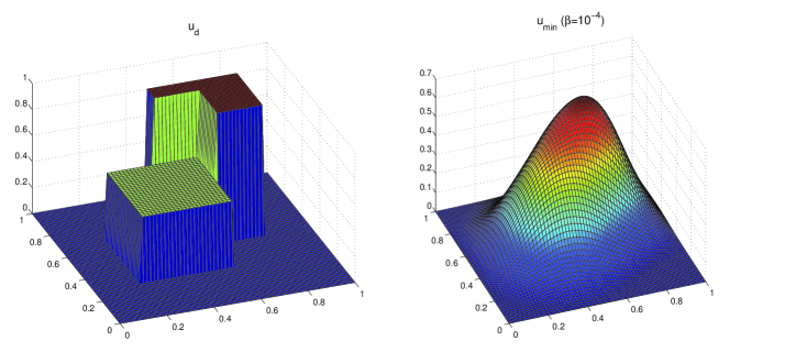
Fig. 3: Left: target control $u_{d}$. Right: optimal control $u_{\min}$ for $\beta=10^{-4}$.

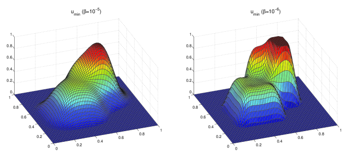
Fig. 4: Left: optimal control $u_{\min}$ for $\beta=10^{-5}$. Right: optimal control $u_{\min}$ for $\beta=10^{-6}$.

Given $n\in\mathbb{N}$, we divide $\Omega$ uniformly in $n^{2}$ squares and we discretize the control space using piecewise constant functions; the departure from the theoretical framework in the earlier sections is minimal, we just replaced triangular elements with rectangular ones. We then use a standard Galerkin formulation to produce a discrete version of ${\mathcal{K}}$ on each grid using continuous bilinear finite elements. Standard finite element analysis (e.g., see [6]) shows that the SAC Condition 1 is satisfied; in particular, part [c] of Condition 1 follows from the $H^{2}$-regularity of the elliptic equation coupled with $L^{\infty}$-convergence (see also [5]). For each

$$n_{j}=64\times 2^{j},\ \ j=0,\dots,6,$$

we initialize the SSNM using the solution obtained from a coarser level; we solve the linear systems in the SSNM solution process using MGCG, and we compare the results against CG. For each run, we report in Tables 1, 2, and 3 the average number of MGCG/CG iterations per SSNM step as well as the added wall-clock times used by the MGCG/CG solves during the entire solution process. The relative tolerance for the linear solves is set at $10^{-8}$. The elliptic problem, i.e., the application of ${\mathcal{K}}_{j}$ and ${\mathcal{K}}_{j}^{*}$ needed for applying the inactive Hessian ${\mathcal{H}}_{j}^{\mathrm{I}}$, is solved numerically using either direct methods (for $n\leqslant 256$) or classical multigrid (the full approximation scheme FAS) using a relative tolerance of $10^{-8}$; the base case for FAS was taken to be $n=256$, a choice that effectively minimized wall-clock times for solving the elliptic problem on our system. For solving the base case (Step 1 in Algorithm 11) in the multigrid preconditioner application we use (unpreconditioned) CG with a matrix-free application of ${\mathcal{H}}_{j_{0}}^{\mathrm{I}}$, and a tolerance of $10^{-10}$. We should emphasize that the multigrid FAS for solving the elliptic problem is used only for applying ${\mathcal{K}}_{j}$ and ${\mathcal{K}}_{j}^{*}$, and is completely independent from the multigrid preconditioner from Algorithm 11, although in the implementation they share part of the infrastructure.

Table 1: Comparison of iteration counts and runtimes for MGCG vs. CG; $\beta=10^{-4}$.

$n_{j}$	$128$	$256$	$512$	$1024$	$2048$	4096	8192
# cg / it.	11.25	11.67	12	12	12	12	12
$t_{\mathrm{cg}}$ (s)	3.65	14	84	427	1915	2.97 h	20.3 h
# mg / it., $j_{0}=0$	5	5	4	4	3	3	3
$t_{\mathrm{mg}}$ (s)	10.5	13.6	100	373	1242	1.41 h	5.97 h
eff=$t_{\mathrm{mg}}/t_{\mathrm{cg}}$	2.87	1.16	1.19	0.87	0.65	0.48	0.29

Table 2: Comparison of iteration counts and runtimes for MGCG vs. CG; $\beta=10^{-5}$.

$n_{j}$	$128$	$256$	$512$	$1024$	$2048$	4096	8192
# cg / it.	20	19.5	19.25	19.75	20	20	20
$t_{\mathrm{cg}}$ (s)	6.24	42	197	793	3081	4.88 h	32.76 h
# mg / it., $j_{0}=0$	7.75	9	8.25	7.75	6	6.67	8
$t_{\mathrm{mg}}$ (s)	15.23	32	257	896	1949	2.28 h	10.84 h
eff=$t_{\mathrm{mg}}/t_{\mathrm{cg}}$	2.44	0.76	1.3	1.12	0.63	0.47	0.33
# mg / it., $j_{0}=1$	-	6.5	7	6	5	4	5
$t_{\mathrm{mg}}$ (s)	-	63	254	796	1865	1.87 h	8.4 h
eff=$t_{\mathrm{mg}}/t_{\mathrm{cg}}$	-	1.5	1.29	1.004	0.605	0.38	0.26

Table 3: Comparison of iteration counts and runtimes for MGCG vs. CG; $\beta=10^{-6}$.

$n_{j}$	$128$	$256$	$512$	$1024$	$2048$	4096	8192
# cg / it.	32.5	31.75	31	31.75	33.25	33	34
$t_{\mathrm{cg}}$ (s)	9.9	48	241	1312	1.92 h	11.72 h	54.58 h
# mg / it., $j_{0}=2$	-	-	9.75	11.75	16	11.25	$>50$
$t_{\mathrm{mg}}$ (s)	-	-	1135	1986	2.06 h	6.98 h	-
$t_{\mathrm{mg}}/t_{\mathrm{cg}}$	-	-	4.71	1.51	1.07	0.59	-
# mg / it., $j_{0}=3$	-	-	-	8.75	10	12	11
$t_{\mathrm{mg}}$ (s)	-	-	-	4155	1.78 h	5.27 h	16.74 h
$t_{\mathrm{mg}}/t_{\mathrm{cg}}$	-	-	-	3.16	0.92	0.45	0.31
# mg / it., $j_{0}=4$	-	-	-	-	6.25	7.75	8.33
$t_{\mathrm{mg}}$ (s)	-	-	-	-	4.61 h	7.69 h	17.44 h
$t_{\mathrm{mg}}/t_{\mathrm{cg}}$	-	-	-	-	2.39	0.66	0.32

First we remark that, for each $\beta$, the SSNM converged in a relatively mesh-independent number of iterations; that number is also independent of the way we solve the linear systems, assuming they are solved to the given tolerance. In the interest of the exposition we do not report the number of SSNM iterations, since the focus is on the linear solves. We also point out that all cases pass the weak test. This is best seen in Table 3 for $\beta=10^{-6}$, where we note the average number of two-grid iterations decreasing from $9.75$ at $n=512$ to $8.75$ at $n=1024$, and down to $6.25$ at $n=2048$; we did not run the two-grid preconditioned problem for $n=4096,8192$. Still for $\beta=10^{-6}$ we see the three-grid average number of iterations decreasing from $11.75$ at $n=1024$ to $10$ at $n=2048$, down to $7.75$ at $n=4096$, and the four-grid average number of iterations decreasing from $16$ at $n=2048$, to $12$ at $n=4096$, down to $8.33$ at $n=8192$.

For the strong test the key issue is the choice of the base case $j_{0}$ for the multigrid preconditioner. The hypotheses of Theorem 15 show that the base level has to be sufficiently fine (relative to $\beta$) in order for MGCG to run efficiently, as shown in (61). In Table 1, for $\beta=10^{-4}$, the choice $j_{0}=0\ (n_{0}=64)$ seems to be sufficiently fine, as the MGCG requires fewer and fewer iterations as $n$ increases, as predicted by theory. The effective efficiency factor eff=time(MGCG) / time (CG) is also presented; it is shown to decrease with increasing resolution, but it decreases below the value one (e.g., MGCG becomes more efficient than CG) only at higher resolution, as expected. For example, at $n=2048$, while CG required an average number of 12 iterations per SSNM iteration (actually exactly 12 at each iteration), the 5-grid MGCG required an average of 3 iterations per SSNM iterations. In terms of wall-clock time, the linear solves for MGCG required 0.65 of the wall-clock time of CG. The situation is somewhat similar for $\beta=10^{-5}$ (Table 2), except for the fact that $j_{0}=0$ turns out to be borderline acceptable, in that the average number of MGCG iterations does not decrease with increasing resolution right from the beginning, so $j_{0}=0$ does not pass the strong test. Instead, the case $j_{0}=1$ $(n_{1}=128)$ clearly passes the strong test with the exception of the mild increase in number of iterations from two-grid to three-grid. Also, the efficiency factor decreases to $0.38$ at $n=4096$ (with a five-grid preconditioner), and further down to $0.26$ at $n=8192$ (with a six-grid preconditioner). Finally, for $\beta=10^{-6}$ (Table 3) we see that neither of the values $j_{0}=2,3,4$ give rise to the expected decrease in the number of iterations for the MGCG, at least not for small number of levels, thus failing the strong test. However, for high-resolution computations MGCG is still more efficient than CG: for example, a five-grid MGCG based solve at $n=8192$ ($j_{0}=3$) requires an average of 11 inner iteration per SSNM iteration and $0.31$ of the time needed for the 34 inner CG iterations per SSNM iteration.

5.2 Image deblurring with box constraints

For the second application we define the restricted Gaussian blurring operator for functions $u\in L^{1}(\mathbb{R}^{2})$ by

$${\mathcal{K}}^{\sigma,w}u(x)=\frac{\alpha_{w}^{-1}}{2\pi}\int_{\lvert x-y\rvert_{\infty}<w}G_{\sigma}(x-y)u(y)dy,$$ (68)

where $\sigma,w>0$, $\lvert x\rvert_{\infty}=\max(\lvert x_{1}\rvert,\lvert x_{2}\rvert)$, $\lvert x\rvert$ is the Euclidean norm,

$$G_{\sigma}(x)=\sigma^{-2}e^{-\frac{|x|^{2}}{2\sigma^{2}}},\ \ \ \ \alpha_{w}=\frac{1}{2\pi}\int_{\lvert x\rvert_{\infty}<w}G_{\sigma}(x)dx\ .$$

Note that $\lim_{w\to\infty}\alpha_{w}=1$. Here $u:\mathbb{R}^{2}\to[0,1]$ is a function representing a grey-scale image. If $D_{w}$ denotes the square $(-w,w)\times(w,w)$ and $\chi_{D_{w}}$ is its characteristic function, then

$${\mathcal{K}}^{\sigma,w}u=\alpha_{w}^{-1}\left(G_{\sigma}\cdot\chi_{D_{w}}\right)*u,$$

where the convolution is defined using the rescaled Lebesgue measure $(2\pi)^{-1}$ (see Appendix A). We remark that in the usual definition of Gaussian blurring, the domain of integration in (68) is the entire space $\mathbb{R}^{2}$. In practice, however, the integral is restricted as shown in (68), the usual choice being $w=3\sigma$, and the “image” $u$ is restricted to a bounded domain $\Omega$. As in the previous section, we consider $\Omega=(0,1)\times(0,1)$, which mainly allows for two options for defining ${\mathcal{K}}^{\sigma,w}$ on $L^{1}(\Omega)$: first we can extend $u\in L^{1}(\Omega)$ with zero outside $\Omega$, case in which ${\mathcal{K}}^{\sigma,w}u$ is defined on the entire space $\mathbb{R}^{2}$; furthermore, we restrict ${\mathcal{K}}^{\sigma,w}u$ to $\Omega$. This gives rise, as shown in Appendix A, to a bounded operator ${\mathcal{K}}^{\sigma,w}\in\mathfrak{L}(L^{2}(\Omega))$. The second option is to not extend $u\in L^{1}(\Omega)$ outside of $\Omega$, which natually results in an operator $\widehat{{\mathcal{K}}}^{\sigma,w}\in\mathfrak{L}(L^{2}(\Omega),L^{2}(\Omega_{w}))$, where $\Omega_{w}=(w,1-w)\times(w,1-w)$ (we require $0<w<1/2$). In our numerical experiments we used a discretization of $\widehat{{\mathcal{K}}}^{\sigma,w}$, while, for convenience, we conduct the analysis in Appendix A for the former case, namely ${\mathcal{K}}^{\sigma,w}$. For the remainder of this section we discard the superscripts $\sigma,w$, i.e., ${\mathcal{K}}={\mathcal{K}}^{\sigma,w}$.

In our numerical solution of the optimization problem (1) we discretize $u$, as before, using piecewise constant functions on a uniform $n\times n$ grid on $\Omega$. With $h=1/n$ being the grid size, we compute the discrete version ${\mathcal{K}}_{h}u$ (representing the blurred image) at the cell centers using a cubature rule to integrate (68) numerically. Essentially, the value of $({\mathcal{K}}_{h}u)$ at a node $z_{k}$ (the center of an element) is a weighted average of the values of $u$ in all squares that are at most $w_{h}$ away from $z_{k}$ (in the $\lvert\>\cdot\>\rvert_{\infty}$-distance), with the weights being computed using the function $G_{\sigma}$ and rescaled to add up to 1; $w_{h}$ is a discrete version of $w$. The details of the discretization, as well as the verification of Condition 1, are given in Appendix A. As customary in Gaussian filtering, the separability of the kernel $G$ allows for a more efficient implementation, namely

$${\mathcal{K}}_{h}={\mathcal{K}}^{x_{1}}_{h}{\mathcal{K}}^{x_{2}}_{h}={\mathcal{K}}^{x_{2}}_{h}{\mathcal{K}}^{x_{1}}_{h}\ ,$$

where ${\mathcal{K}}^{x_{1}}_{h}u$ (resp., ${\mathcal{K}}^{x_{2}}_{h}u$) defines the application of a Gaussian filter to the image $u$ in the $x_{1}$-direction only (resp., $x_{2}$-direction).

The setup and result presentation is similar to the experiments presented in Section 5.1. We consider the case when $w=0.1$ and $\sigma=w/3$. Again, we define the data by $y_{d}={\mathcal{K}}u_{d}$, where the target control $u_{d}$, i.e., the original image (shown as a surface), is the same step function as in the previous experiment. In Figure 5 we show both $u_{d}$ (left) and the blurred image $y_{d}={\mathcal{K}}u_{d}$ (right) as surfaces. For the constrained optimization problem we use the constant constraints $a(x)=0$ and $b(x)=1$. In Figures 6 and 7 we show the solutions of the constrained problem for $\beta=0.04,0.02,0.01,0.005$.

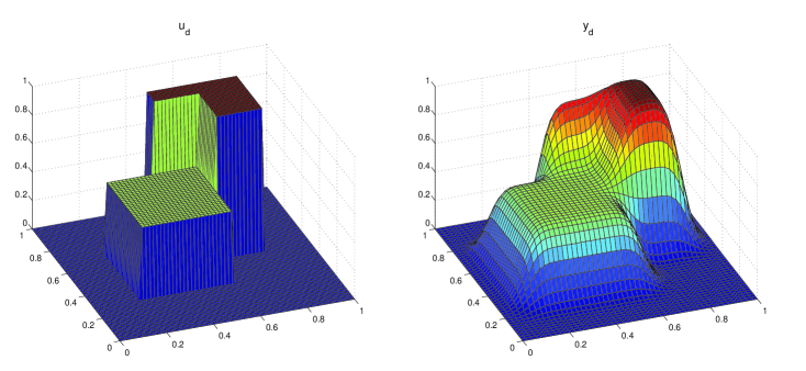
Fig. 5: Left: target control $u_{d}$. Right: blurred image/surface $y_{d}$.

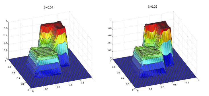
Fig. 6: Left: optimal control $u_{\min}$ for $\beta=0.04$. Right: optimal control $u_{\min}$ for $\beta=0.02$.

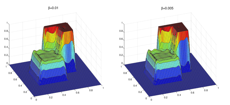
Fig. 7: Left: optimal control $u_{\min}$ for $\beta=0.01$. Right: optimal control $u_{\min}$ for $\beta=0.005$.

Table 4: Comparison of iteration counts and runtimes for multigrid vs. unpreconditioned CG for image deblurring; $w=0.1,\beta=0.04,0.02$.

$n_{j}$	$256$	$512$	$1024$	$2048$
$\beta=0.04$
# cg / it.	40	40	40	40
$t_{\mathrm{cg}}$ (s)	3.6	25	215	4023
# mg / it., $j_{0}=0$	12.2	14.5	21	12.5
$t_{\mathrm{mg}}$ (s)	7.2	18	149	1442
# mg / it., $j_{0}=1$	-	9.25	11.5	10.25
$t_{\mathrm{mg}}$ (s)	-	39	101	1240
# mg / it., $j_{0}=2$	-	-	7.5	8.75
$t_{\mathrm{mg}}$ (s)	-	-	290	1347
# mg / it., $j_{0}=3$	-	-	-	6.5
$t_{\mathrm{mg}}$ (s)	-	-	-	2665
$\beta=0.02$
# cg / it.	51.2	51	51	51
$t_{\mathrm{cg}}$ (s)	4.6	32	270	5354
# mg / it., $j_{0}=0$	15.8	18.75	61.75	57
$t_{\mathrm{mg}}$ (s)	12	23	450	6256
# mg / it., $j_{0}=1$	-	11	14	23.75
$t_{\mathrm{mg}}$ (s)	-	53	142	2797
# mg / it., $j_{0}=2$	-	-	9.5	11.75
$t_{\mathrm{mg}}$ (s)	-	-	418	1682
# mg / it., $j_{0}=3$	-	-		7.25
$t_{\mathrm{mg}}$ (s)	-	-	-	3072

Table 5: Comparison of iteration counts and runtimes for multigrid vs. unpreconditioned CG for image deblurring; $w=0.1,\beta=0.01,0.005$.

$n_{j}$	$256$	$512$	$1024$	$2048$
$\beta=0.01$
# cg / it.	65.8	66	66	66
$t_{\mathrm{cg}}$ (s)	6	60	446	6576
# mg / it., $j_{0}=0$	20.8	25.2	$>100$	$>100$
$t_{\mathrm{mg}}$ (s)	18	46
# mg / it., $j_{0}=1$	-	15.4	19.8	$>100$
$t_{\mathrm{mg}}$ (s)	-	119	279
# mg / it., $j_{0}=2$	-	-	11.8	15.5
$t_{\mathrm{mg}}$ (s)	-	-	846	2316
# mg / it., $j_{0}=3$	-	-	-	9
$t_{\mathrm{mg}}$ (s)	-	-	-	4390
$\beta=0.005$
# cg / it.	84.67	84.25	84.6	84.74
$t_{\mathrm{cg}}$ (s)	9	52	560	8926
# mg / it., $j_{0}=0$	31.5	37.5	failed	failed
$t_{\mathrm{mg}}$ (s)	42	64	-	-
# mg / it., $j_{0}=1$	-	19.75	26.2	failed
$t_{\mathrm{mg}}$ (s)	-	152	402	-
# mg / it., $j_{0}=2$	-	-	15.2	20.25
$t_{\mathrm{mg}}$ (s)	-	-	1218	3260
# mg / it., $j_{0}=3$	-	-	-	11.5
$t_{\mathrm{mg}}$ (s)	-	-	-	6779

For the multigrid solves we consider the cases

$$n_{j}=128\times 2^{j},\ \ j=0,\dots,4.$$

We report the results for $\beta=0.04,~{}0.02$ in Table 4 and for $\beta=0.01,~{}0.005$ in Table 5, but we no longer report the effective efficiency factor.

The results are essentially similar with the elliptic-constrained experiments. All cases clearly pass the weak test. However, the only case where there is a hint of the strong test being passed is for $\beta=0.04$ (top half of Table 4); for $j_{0}=0$ we see the average number of iterations first increasing with resolution from $12.2$ ($n_{1}=256$) to $14.5$ ($n_{2}=512$) up to $21$ ($n_{3}=1024$), only to decrease to $12.5$ for ($n_{4}=2048$), all compared to an average number of $40$ CG iterations. This certainly reflected in the wall-clock efficiency: the five-level MGCG linear solves required 1442 seconds compared to the 4023 seconds for CG.

As in the elliptic-constrained experiments, by lowering $\beta$ to $0.02$ (bottom half of Table 4) we also have to raise the base case level in order for MGCG to run efficiently; here $j_{0}=2$ seems to be sufficiently fine, but even $j_{0}=1$ seems to be acceptable, i.e., lead to reasonably efficient linear solves. By contrast we see how even lower values for $\beta$ (see Table 5) lead to very slowly convergent linear solves (see the cases $\beta=0.01$ and $j_{0}=0,1$) or even non-convergence ($\beta=0.005$ and $j_{0}=0,1$).

6 Conclusions

We have developed a multigrid preconditioning technique to be used in connection to SSNMs for certain control-constrained distributed optimal control problems. The multigrid preconditioners exhibit a provably optimal order behavior with respect to the mesh-size, in that the quality of the preconditioners increases at the optimal rate with increasing mesh-size, assuming a piecewise constant representation of the control and a sufficiently fine base level. The technique used in this paper is not limited to control-constrained problems like (1). An immediate application would be to replace (or add) a domain-constraint to the control $u$ of the type supp($u)\subseteq\Omega^{\prime}$, where $\Omega^{\prime}\subset\Omega$. Naturally, our method can be also used for PDE-constrained optimization with state constraints by reducing them to control-constrained problem via Lavrentiev regularization.

A natural question is whether the method can be extended to higher order discontinuous piecewise polynomial discretizations such that the optimality of the preconditioner is preserved. Following the analysis of the piecewise constant case, it is apparent that the answer is negative. However, this does not preclude the existence of alternate optimal order preconditioners for higher order discretizations of the controls. The search for such preconditioners is subject of ongoing research.

Appendix A Verification of Condition SAC for the restricted Gaussian blurring operator

In this section we rigorously specify the discretization for the integral operator ${\mathcal{K}}^{\sigma,w}$ defined in Section 5.2, and we show that Condition 1 is satisfied. Recall that $\Omega=(0,1)\times(0,1)$ with $0<w<1/2$.

A.1 Estimates for the continous operator

Due to the definition of ${\mathcal{K}}^{\sigma,w}$ as a convolution, we prefer to verify Condition 1 [a] using Fourier transforms. Following [21], we consider the normalized Lebesgue measure on $\mathbb{R}^{n}$ defined by

$$dm_{n}(x)=(2\pi)^{-n/2}dx\ ,$$

and we define the Fourier transform of a function $f\in L^{1}(\mathbb{R}^{n})$ by

$${\mathcal{F}}_{n}[f](\xi)=\int_{\mathbb{R}^{n}}f(x)e^{-{\bf i}\>\xi\cdot x}dm_{n}(x)\ .$$

In this section $L^{2}$-norms of functions in $\mathbb{R}^{n}$ or on bounded domains, as well as convolutions, are computed using the measure $dm_{n}$, i.e.,

$$|\!|f|\!|^{2}_{L^{2}(\mathbb{R}^{n})}=\int_{\mathbb{R}^{n}}\lvert f(x)\rvert^{2}dm_{n}(x),\ \ \ (f*g)(x)\stackrel{{\scriptstyle\mathrm{def}}}{{=}}\int_{\mathbb{R}^{n}}f(x-y)\>g(y)dm_{n}(y)\ .$$

Lemma 17.

There exists a constants $C_{1},C_{2},C_{3}$ depending only on the ratio $w/\sigma$ so that

$$\left|{\mathcal{F}}_{1}[\chi_{(-w,w)}(x)\cdot e^{-\frac{x^{2}}{2\sigma^{2}}}](\xi)\right|\leqslant\min\left(C_{1}/\lvert\xi\rvert,\ \sigma\>C_{2}\right)\ ,\ \ \forall\xi\neq 0,$$ (69)

and

$$\left|{\mathcal{F}}_{1}[\chi_{(-w,w)}(x)\cdot e^{-\frac{x^{2}}{2\sigma^{2}}}](\xi)\right|\leqslant\frac{\sigma C_{3}}{1+\sigma\left|\xi\right|}\ ,\ \ \forall\xi\in\mathbb{R}.$$ (70)

Proof.

Cf. [21], for $\xi\in\mathbb{R}$ the following hold:

$${\mathcal{F}}_{1}[\chi_{(-w,w)}(x)](\xi) = \sqrt{\frac{2}{\pi}}\>\frac{\sin(w\>\xi)}{\xi}\ \ \mathrm{and}\ \ {\mathcal{F}}_{1}[e^{-\frac{x^{2}}{2\sigma^{2}}}](\xi)=\sigma\>e^{-\frac{(\sigma\xi)^{2}}{2}}\ ,$$

where $\sin(w\xi)/\xi$ is continued analytically at $\xi=0$. It follows that

$$(\sigma^{-1}\>\pi)\left|{\mathcal{F}}_{1}[\chi_{(-w,w)}(x)\cdot e^{-\frac{x^{2}}{2\sigma^{2}}}](\xi)\right|$$ (71)

$$= \sqrt{2\pi}\>\left|e^{-\frac{(\sigma\xi)^{2}}{2}}*\frac{\sin(w\>\xi)}{\xi}\right|=\left|\int_{-\infty}^{\infty}e^{-\frac{(\sigma(\xi-\zeta))^{2}}{2}}\cdot\frac{\sin(w\>\zeta)}{\zeta}d\zeta\right|$$

$$\underset{\sigma\xi=s}{\overset{\sigma\zeta=t}{=}} \left|\int_{-\infty}^{\infty}e^{-\frac{(s-t)^{2}}{2}}\cdot\frac{\sin(\sigma^{-1}wt)}{t}dt\right|\ .$$

Since $\left|\sin(at)/t\right|\leqslant\lvert a\rvert$, we obtain

$$(\sigma^{-1}\>\pi)\left|{\mathcal{F}}_{1}[\chi_{(-w,w)}(x)\cdot e^{-\frac{x^{2}}{2\sigma^{2}}}](\xi)\right| \leqslant \sigma^{-1}w\left|\int_{-\infty}^{\infty}e^{-\frac{(s-t)^{2}}{2}}dt\right|=\sqrt{2\pi}\sigma^{-1}w\ ,$$

so in (69) we can take $C_{2}=\sigma^{-1}w\sqrt{2/\pi}$. For computing $C_{1}$, let $\delta\in(0,1)$, and recall $\sigma\>\xi=s$. Without loss of generality assume $\xi>0$. Continuing from (71),

$$(\sigma^{-1}\>\pi)\left|{\mathcal{F}}_{1}[\chi_{(-w,w)}(x)\cdot e^{-\frac{x^{2}}{2\sigma^{2}}}](\xi)\right|$$

$$\leqslant \left|\int_{\lvert s-t\rvert<s\>\delta}e^{-\frac{(s-t)^{2}}{2}}\cdot\frac{\sin(\sigma^{-1}wt)}{t}dt\right|+\left|\int_{\lvert s-t\rvert>s\>\delta}e^{-\frac{(s-t)^{2}}{2}}\cdot\frac{\sin(\sigma^{-1}wt)}{t}dt\right|$$

$$\leqslant \frac{1}{s(1-\delta)}\int_{\lvert s-t\rvert<s\>\delta}e^{-\frac{(s-t)^{2}}{2}}dt+(\sigma^{-1}w)\int_{\lvert s-t\rvert>s\>\delta}e^{-\frac{(s-t)^{2}}{2}}dt$$

$$\stackrel{{\scriptstyle s-t=u}}{{\leqslant}} \frac{1}{s(1-\delta)}\int_{-\infty}^{\infty}e^{-\frac{u^{2}}{2}}du+(\sigma^{-1}w)\int_{\lvert u\rvert>s\>\delta}e^{-\frac{u^{2}}{2}}du$$

$$\leqslant \frac{\sqrt{2\pi}}{s(1-\delta)}+2(\sigma^{-1}w)\int^{\infty}_{s\>\delta}e^{-\frac{s\delta}{2}u}du=\frac{\sqrt{2\pi}}{s(1-\delta)}+4\frac{(\sigma^{-1}w)}{s\>\delta}e^{-\frac{(s\delta)^{2}}{2}}$$

$$\leqslant \left(\sigma\xi\right)^{-1}\left(\frac{\sqrt{2\pi}}{1-\delta}+\frac{4\sigma^{-1}w}{\delta}\right)\ .$$

The choice $\delta=1/2$ shows that in (69) we can take $C_{1}=2\pi^{-1}\left({\sqrt{2\pi}}+4\sigma^{-1}w\right)$. It is easy to see that for $a_{1},a_{2},b>0$

$$\min\left(\frac{a_{1}}{\left|\xi\right|},a_{2}\right)\leqslant\frac{a_{1}+a_{2}b}{b+\left|\xi\right|}\ .$$ (72)

Hence, the inequality (70) follows from (69) by substituting $a_{1}=C_{1}$, $a_{2}=\sigma C_{2}$, and $b=1/\sigma$ in (72), with $C_{3}=C_{1}+C_{2}$. ∎

The next Lemma shows that ${\mathcal{K}}^{\sigma,w}$ satisfies Condition 1 [a] (recall that the operator is symmetric).

Lemma 18.

There exists a constant $C>0$ depending on the ratio $w/\sigma$ so that

$$|\!|{\mathcal{K}}^{\sigma,w}u|\!|_{L^{2}(\mathbb{R}^{2})} \leqslant C\alpha_{w}^{-1}|\!|u|\!|,\ \ \forall u\in L^{2}(\mathbb{R}^{2})\ ,$$ (73)

$$|\!|{\mathcal{K}}^{\sigma,w}u|\!|_{L^{2}(\Omega)} \leqslant C\alpha_{w}^{-1}|\!|u|\!|,\ \ \forall u\in L^{2}(\Omega)\ ,$$ (74)

$$|\!|{\mathcal{K}}^{\sigma,w}u|\!|_{H^{1}(\mathbb{R}^{2})} \leqslant \alpha_{w}^{-1}\left(C\max(1,\sigma^{-1})\right)|\!|u|\!|,\ \ \forall u\in L^{2}(\mathbb{R}^{2})\ ,$$ (75)

$$|\!|{\mathcal{K}}^{\sigma,w}u|\!|_{H^{1}(\Omega)} \leqslant \alpha_{w}^{-1}\left(C\max(1,\sigma^{-1})\right)|\!|u|\!|,\ \ \forall u\in L^{2}(\Omega)\ .$$ (76)

Proof.

Cf. [21], an equivalent $H^{k}$-norm of a function $v$ on $\mathbb{R}^{2}$ is given by

$$|\!|v|\!|_{H^{k}(\mathbb{R}^{2})}=|\!|L_{k}\cdot{\mathcal{F}}_{2}[v]|\!|,$$

where $L_{k}(\xi)=(1+\lvert\xi\rvert^{2})^{\frac{k}{2}}$ for $k\geqslant 0$. Hence, for $u\in L^{2}(\mathbb{R}^{2})$ and $k=0,1$

$$\alpha_{w}|\!|{\mathcal{K}}^{\sigma,w}u|\!|_{H^{k}(\mathbb{R}^{2})} = |\!|L_{k}\cdot{\mathcal{F}}_{2}[\left(G_{\sigma}\cdot\chi_{D_{w}}\right)*u]|\!|=|\!|L_{k}\cdot{\mathcal{F}}_{2}[G_{\sigma}\cdot\chi_{D_{w}}]\cdot{\mathcal{F}}_{2}[u]|\!|$$

$$\leqslant |\!|L_{k}\cdot{\mathcal{F}}_{2}[G_{\sigma}\cdot\chi_{D_{w}}]|\!|_{L^{\infty}(\mathbb{R}^{2})}\cdot|\!|{\mathcal{F}}_{2}[u]|\!|\ .$$ (77)

By the Plancherel Theorem, $|\!|{\mathcal{F}}_{2}[u]|\!|=|\!|u|\!|$; hence, it remains to estimate the quantity

$$|\!|L_{k}\cdot{\mathcal{F}}_{2}[G_{\sigma}\cdot\chi_{D_{w}}]|\!|_{L^{\infty}(\mathbb{R}^{2})}.$$ (78)

The separability

$$(G_{\sigma}\cdot\chi_{D_{w}})(x_{1},x_{2})=\sigma^{-2}\left(e^{-\frac{{x_{1}}^{2}}{2\sigma^{2}}}\chi_{(-w,w)}(x_{1})\right)\cdot\left(e^{-\frac{{x_{2}}^{2}}{2\sigma^{2}}}\chi_{(-w,w)}(x_{2})\right)$$

implies that

$${\mathcal{F}}_{2}[G_{\sigma}\cdot\chi_{D_{w}}](\xi_{1},\xi_{2}) =\sigma^{-2}{\mathcal{F}}_{1}[e^{-\frac{{x_{1}}^{2}}{2\sigma^{2}}}\chi_{(-w,w)}(x_{1})](\xi_{1})\cdot{\mathcal{F}}_{1}[e^{-\frac{{x_{2}}^{2}}{2\sigma^{2}}}\chi_{(-w,w)}(x_{2})](\xi_{2}).$$

The case $k=0$ is easy, since by (70)

$$|\!|L_{0}\cdot{\mathcal{F}}_{2}[G_{\sigma}\cdot\chi_{D_{w}}]|\!|_{L^{\infty}(\mathbb{R}^{2})}=|\!|{\mathcal{F}}_{2}[G_{\sigma}\cdot\chi_{D_{w}}]|\!|_{L^{\infty}(\mathbb{R}^{2})}\leqslant(C_{3})^{2}\ ,$$

which, in light of (77), proves (73), and hence (74).

For $k=1$, we have

$$\left|\left(L_{1}\cdot{\mathcal{F}}_{2}[G_{\sigma}\cdot\chi_{D_{w}}\right)(\xi_{1},\xi_{2})]\right| = \left|(1+\xi_{1}^{2}+\xi_{2}^{2})^{\frac{1}{2}}{\mathcal{F}}_{2}[G_{\sigma}\cdot\chi_{D_{w}}](\xi_{1},\xi_{2})\right|$$

$$\stackrel{{\scriptstyle\eqref{eq:ftlinfnorm2}}}{{\leqslant}} (C_{3})^{2}\frac{\sqrt{1+\xi_{1}^{2}+\xi_{2}^{2}}}{(1+\sigma\lvert\xi_{1}\rvert)(1+\sigma\lvert\xi_{2}\rvert)}$$

$$\leqslant (C_{3})^{2}\max(1,\sigma^{-1})\ .$$

The latter inequality follows from

$$\frac{\sqrt{A+t^{2}}}{1+\sigma t}\leqslant\max(\sqrt{A},\sigma^{-1}),\ \ \forall\ A,\sigma>0,\ t\geqslant 0\ .$$ (79)

Namely, for all $\xi_{1},\xi_{2}\in\mathbb{R}$,

$$\frac{\sqrt{1+\xi_{1}^{2}+\xi_{2}^{2}}}{(1+\sigma\lvert\xi_{1}\rvert)(1+\sigma\lvert\xi_{2}\rvert)} \stackrel{{\scriptstyle\eqref{eq:Asigineq}}}{{\leqslant}} \frac{1}{1+\sigma\lvert\xi_{2}\rvert}\max\left(\sqrt{1+\xi_{2}^{2}},\sigma^{-1}\right)$$

$$\stackrel{{\scriptstyle\eqref{eq:Asigineq}}}{{\leqslant}} \max\left(\max\left(1,\sigma^{-1}\right),\frac{\sigma^{-1}}{1+\sigma\lvert\xi_{2}\rvert}\right)=\max(1,\sigma^{-1})\ .$$

This proves that

$$|\!|L_{1}\cdot{\mathcal{F}}_{2}[G_{\sigma}\cdot\chi_{D_{w}}]|\!|_{L^{\infty}(\mathbb{R}^{2})}\leqslant(C_{3})^{2}\max(1,\sigma^{-1}),$$ (80)

thus showing that (75) holds with $C=(C_{3})^{2}$.

Given $u\in L^{2}(\Omega)$, we consider its extension (still denoted $u$) with $0$ outside $\Omega$, and we apply the inequality (75) to obtain

$$|\!|{\mathcal{K}}^{\sigma,w}u|\!|_{H^{1}(\Omega)} \leqslant |\!|{\mathcal{K}}^{\sigma,w}u|\!|_{H^{1}(\mathbb{R}^{2})}$$

$$\leqslant \alpha_{w}^{-1}\left(C\max(1,\sigma^{-1})\right)|\!|u|\!|_{L^{2}(\mathbb{R}^{2})}=\alpha_{w}^{-1}\left(C\max(1,\sigma^{-1})\right)|\!|u|\!|_{L^{2}(\Omega)}\ ,$$

which proves (76). ∎

Lemma 19.

If $0<w_{0}\leqslant w_{1}<w_{2}<1/2$, then

$$|\!|({\mathcal{K}}^{\sigma,w_{1}}-{\mathcal{K}}^{\sigma,w_{2}})u|\!|_{L^{2}(\mathbb{R}^{2})} \leqslant C\>(w_{2}-w_{1})|\!|u|\!|_{L^{2}(\mathbb{R}^{2})}\ ,$$ (81)

$$|\!|({\mathcal{K}}^{\sigma,w_{1}}-{\mathcal{K}}^{\sigma,w_{2}})u|\!|_{L^{2}(\Omega)} \leqslant C\>(w_{2}-w_{1})|\!|u|\!|_{L^{2}(\Omega)}\ ,$$ (82)

where the constant $C$ only depends on $\sigma$ and $w_{0}$.

Proof.

Since $w_{0}\leqslant w_{1}<w_{2}$, it follows that $D_{w_{0}}\subseteq D_{w_{1}}\subset D_{w_{2}}$. Let $D_{w_{1},w_{2}}=D_{w_{2}}\setminus D_{w_{1}}$. Because $w_{1}+w_{2}<1$,

$$\mu(D_{w_{1},w_{2}})=4(w_{2}^{2}-w_{1}^{2})<4(w_{2}-w_{1})\ .$$

Also,

$$\alpha_{w_{2}}-\alpha_{w_{1}}=\frac{1}{2\pi}\int_{D_{w_{1},w_{2}}}G_{\sigma}(x)dx\leqslant\frac{2(w_{2}-w_{1})}{\pi}\>\left|\!\left|G_{\sigma}\right|\!\right|_{L^{\infty}(\mathbb{R}^{2})}=\frac{2(w_{2}-w_{1})}{\sigma^{2}\pi}\ .$$

Therefore

$$\alpha_{w_{1}}^{-1}-\alpha_{w_{2}}^{-1}=\frac{\alpha_{w_{2}}-\alpha_{w_{1}}}{\alpha_{w_{1}}\>\alpha_{w_{2}}}\leqslant\frac{2(w_{2}-w_{1})}{\alpha_{w_{0}}^{2}\sigma^{2}\pi}\stackrel{{\scriptstyle\mathrm{def}}}{{=}}{c_{1}}(w_{2}-w_{1})\ ,$$

since $\alpha_{w_{2}}>\alpha_{w_{1}}\geqslant\alpha_{w_{0}}$. For $u\in L^{2}(\mathbb{R}^{2})$

$$|\!|({\mathcal{K}}^{\sigma,w_{2}}-{\mathcal{K}}^{\sigma,w_{1}})u|\!|_{L^{2}(\mathbb{R}^{2})}$$

$$= |\!|\left(\alpha_{w_{2}}^{-1}G_{\sigma}(\chi_{D_{w_{2}}}-\chi_{D_{w_{1}}})+(\alpha_{w_{2}}^{-1}-\alpha_{w_{1}}^{-1})G_{\sigma}\cdot\chi_{D_{w_{1}}}\right)*u|\!|_{L^{2}(\mathbb{R}^{2})}$$

$$\leqslant \alpha_{w_{2}}^{-1}|\!|(G_{\sigma}\cdot\chi_{D_{w_{1},w_{2}}})*u|\!|_{L^{2}(\mathbb{R}^{2})}+\lvert\alpha_{w_{2}}^{-1}-\alpha_{w_{1}}^{-1}\rvert\cdot|\!|(G_{\sigma}\cdot\chi_{D_{w_{1}}})*u|\!|_{L^{2}(\mathbb{R}^{2})}$$

$$\leqslant \left(\alpha_{w_{2}}^{-1}|\!|G_{\sigma}\cdot\chi_{D_{w_{1},w_{2}}}|\!|_{L^{1}(\mathbb{R}^{2})}+\lvert\alpha_{w_{2}}^{-1}-\alpha_{w_{1}}^{-1}\rvert\cdot|\!|G_{\sigma}\cdot\chi_{D_{w_{1}}}|\!|_{L^{1}(\mathbb{R}^{2})}\right)|\!|u|\!|_{L^{2}(\mathbb{R}^{2})}\hskip 30.0pt$$

$$\leqslant |\!|G_{\sigma}|\!|_{L^{\infty}(\mathbb{R}^{2})}\left(\alpha_{w_{2}}^{-1}\cdot\mu(D_{w_{1},w_{2}})+c_{1}(w_{2}-w_{1})\mu(D_{w_{1}})\right)\cdot|\!|u|\!|_{L^{2}(\mathbb{R}^{2})}$$

$$\leqslant \sigma^{-2}\left(4\alpha_{w_{0}}^{-1}+c_{1}\right)(w_{2}-w_{1})|\!|u|\!|_{L^{2}(\mathbb{R}^{2})}\stackrel{{\scriptstyle\mathrm{def}}}{{=}}C(w_{2}-w_{1})|\!|u|\!|_{L^{2}(\mathbb{R}^{2})}\ ,$$

where in (A.1) we used Young’s inequality for convolutions. Naturally, $C$ only depends on $\sigma$ and $w_{0}$. As before, the inequality (82) follows from (81) by extending $u\in L^{2}(\Omega)$ with zero outside $\Omega$. ∎

A.2 The discretization of ${\mathcal{K}}^{\sigma,w}$ and convergence estimates

Recall that the domain $\Omega$ is partitioned uniformly into $N_{h}=n^{2}$ squares $\Omega=\cup_{k=1}^{N_{h}}R_{k}$ with $h=1/n$, and let $z_{k}$ be the center of the square $R_{k}$. We denote by ${\mathcal{U}}_{h}$ the space of piecewise constant functions on $\Omega$ with respect to the aforementioned partition, with functions in ${\mathcal{U}}_{h}$ being determined by their values at the nodes $z_{k}$. For this example we take ${\mathcal{V}}_{h}={\mathcal{U}}_{h}$, so ${\mathcal{K}}_{h}\in\mathfrak{L}({\mathcal{U}}_{h})$. Note that ${\mathcal{V}}_{h}\not\subset H^{1}({\Omega})$. For convenience and consistency with the continuous case we extend the grid to $\mathbb{R}^{2}$ and we extend any function in ${\mathcal{U}}_{h}$ with zero outside $\Omega$. In this section $|\!|\cdot|\!|$ denotes the $L^{2}$-norm on $\Omega$.

The first step towards discretization is to slightly enlarge the domain of integration in (68), when $x=z_{k}$, to be a union of elements in the partition. Hence, for a given node $z_{k}$, denote by ${\mathcal{N}}_{k}$ the set of indices $l$ for which Int$(R_{k})$ intersects the ball ${\mathcal{B}}_{w}(z_{k})=\{y\in\Omega\>:\>\lvert y-z_{k}\rvert_{\infty}<w\}$. It is easy to see that

$${\mathcal{N}}_{k}=\left\{l\>:\>\lvert z_{k}-z_{l}\rvert_{\infty}\leqslant w(1+h/2)\right\}\ .$$

So for $x=z_{k}$ the domain of integration in (68) becomes

$$\bigcup_{l\in{\mathcal{N}}_{k}}R_{l}={\mathcal{B}}_{w_{h}}(z_{k})\ ,\ \ \ \mathrm{with}\ \ w_{h}\stackrel{{\scriptstyle\mathrm{def}}}{{=}}\left(\left\lceil\frac{w}{h}-\frac{1}{2}\right\rceil+\frac{1}{2}\right)h.$$

Essentially, this is the smallest ball (in the $\lvert\>\cdot\>\rvert_{\infty}$-norm) centered at $z_{k}$ that includes ${\mathcal{B}}_{w}(z_{k})$ and is also a union of mesh-elements. Note that

$$w\leqslant w_{h}<w+h\ .$$ (84)

The discretization ${\mathcal{K}}_{h}\in\mathfrak{L}({\mathcal{U}}_{h})$ of ${\mathcal{K}}={\mathcal{K}}^{\sigma,w}$ is given by

$$({{\mathcal{K}}}_{h}u)(z_{k})\stackrel{{\scriptstyle\mathrm{def}}}{{=}}(1+\eta)\>\sum_{l\in{\mathcal{N}}_{k}}{\gamma}_{kl}\>u(z_{l})\stackrel{{\scriptstyle\mathrm{def}}}{{=}}(1+\eta)(\widetilde{K}_{h}u)(z_{k})$$ (85)

with ${\gamma}_{kl}=h^{2}(2\alpha_{w_{h}}\pi)^{-1}G_{\sigma}(z_{k}-z_{l})$, where $\eta$ is chosen so that

$$(1+\eta)\sum_{l\in{\mathcal{N}}_{k}}{\gamma}_{kl}=1\ ,$$ (86)

for all $1\leqslant k\leqslant N_{h}$ for which ${\mathcal{B}}_{w_{h}}(z_{k})\subseteq\Omega$. Note that due to the uniformity of the grid, ${\gamma}_{kl}$ only depends on the vector $(z_{k}-z_{l})$. The next result shows that the operators ${\mathcal{K}}^{\sigma,w}$ and ${{\mathcal{K}}}_{h}$ satifsy Condition 1[b] and [c].

Theorem 20.

There exists a constant $C>0$ which depends on $\sigma,w$ so that

$$|\!|({\mathcal{K}}^{\sigma,w}-{{\mathcal{K}}}_{h})u|\!| \leqslant Ch|\!|u|\!|,\ \ \forall u\in{\mathcal{U}}_{h}$$ (87)

$$|\!|{{\mathcal{K}}}_{h}u|\!|_{L^{\infty}(\Omega)} \leqslant C|\!|u|\!|,\ \ \forall u\in{\mathcal{U}}_{h}\ ,$$ (88)

assuming $h$ is sufficiently small.

Proof.

Throughout this analysis $C$ denotes a generic positive constant depending on $\sigma,w$ but not on $h$. By Lemma 19

$$|\!|({\mathcal{K}}^{\sigma,w}-{\mathcal{K}}^{\sigma,w_{h}})u|\!|\leqslant C(w_{h}-w)|\!|u|\!|\stackrel{{\scriptstyle\eqref{eq:wdiff}}}{{\leqslant}}Ch|\!|u|\!|,\ \ \forall u\in{\mathcal{U}}_{h}\ .$$ (89)

Let ${\mathcal{I}}_{h}:L^{2}(\Omega)\to{\mathcal{U}}_{h}$ be the interpolation operator

$$({\mathcal{I}}_{h}v)(z_{k})=\frac{1}{\mu(R_{k})}\int_{R_{k}}v(x)dx\ .$$

By the Bramble-Hilbert Lemma and Lemma 18

$$|\!|({\mathcal{K}}^{\sigma,w_{h}}-{\mathcal{I}}_{h}{\mathcal{K}}^{\sigma,w_{h}})u|\!|\leqslant Ch|\!|{\mathcal{K}}^{\sigma,w_{h}}u|\!|_{1}\leqslant Ch|\!|u|\!|,\ \ \forall u\in{\mathcal{U}}_{h}\ ,$$ (90)

with $C$ depending only on $w_{h}/\sigma$ and the domain $\Omega$; hence $C$ can be bounded uniformly with respect to $h$. We now fix an index $1\leqslant k\leqslant N_{h}$, and let $l\in{\mathcal{N}}_{k}$. The choice ${\gamma}_{kl}$ is so that $(\widetilde{K}_{h}u)(z_{k})$ is obtained by replacing in (68) (with $w_{h}$ instead of $w$ and $x=z_{k}$) the integral on each $R_{l}$ ($l\in{\mathcal{N}}_{k}$) by the midpoint cubature. Therefore, since $u$ is constant on each $R_{l}$,

$$({\mathcal{K}}^{\sigma,w_{h}}-\widetilde{K}_{h})u(z_{k})=\frac{\alpha_{w_{h}}^{-1}}{2\pi}\sum_{l\in{\mathcal{N}}_{k}}\int_{R_{l}}\left(G_{\sigma}(z_{k}-y)-G_{\sigma}(z_{k}-z_{l})\right)u(z_{l})dy.\hskip 30.0pt$$ (91)

Let $M_{\sigma}$ be the upper bound of the second order (bilinear) Fréchet differential of $G_{\sigma}$, regarded as a function from $(\mathbb{R}^{2},\lvert\>\cdot\>\rvert_{\infty})$ to $\mathbb{R}$ (it is easy to see that all differentials of $G_{\sigma}$ are bounded uniformly on $\mathbb{R}^{2}$). Then the Taylor expansion of the function $y\mapsto G_{\sigma}(z_{k}-y)$ around $z_{l}$ gives

$$\lvert G_{\sigma}(z_{k}-y)-G_{\sigma}(z_{k}-z_{l})+dG_{\sigma}(z_{k})(y-z_{l})\rvert_{\infty}\leqslant\frac{M_{\sigma}}{2}\lvert y-z_{l}\rvert^{2}\ .$$

Due to the symmetry of $R_{l}$ with respect to $z_{l}$ we have

$$\int_{R_{l}}dG_{\sigma}(z_{k})(y-z_{l})dy=0\ .$$

Hence

$$\left|\int_{R_{l}}\left(G_{\sigma}(z_{k}-y)-G_{\sigma}(z_{k}-z_{l})\right)dy\right|\leqslant\mu(R_{l})\frac{M_{\sigma}h^{2}}{2}\ .$$ (92)

By (91) and (92)

$$\left|({\mathcal{K}}^{\sigma,w_{h}}-\widetilde{K}_{h})u(z_{k})\right|\leqslant h^{2}\frac{\alpha_{w_{h}}^{-1}M_{\sigma}}{4\pi}\sum_{l\in{\mathcal{N}}_{k}}\mu(R_{l})\lvert u(z_{l})\rvert\leqslant h^{2}\frac{\alpha_{w}^{-1}M_{\sigma}}{4\pi}|\!|u|\!|_{L^{1}(\Omega)}.\hskip 30.0pt$$ (93)

Using the continuous inclusions $L^{\infty}\subset L^{2}\subset L^{1}$

$$|\!|({\mathcal{I}}_{h}{\mathcal{K}}^{\sigma,w_{h}}-\widetilde{K}_{h})u|\!|\leqslant C|\!|({\mathcal{I}}_{h}{\mathcal{K}}^{\sigma,w_{h}}-\widetilde{K}_{h})u|\!|_{L^{\infty}(\Omega)}\stackrel{{\scriptstyle\eqref{eq:pointwiseest}}}{{\leqslant}}Ch^{2}|\!|u|\!|_{L^{1}(\Omega)}\leqslant Ch^{2}|\!|u|\!|.\hskip 30.0pt$$ (94)

The estimates (89), (90), and (94) imply that

$$|\!|({\mathcal{K}}^{\sigma,w}-{\widetilde{{\mathcal{K}}}}_{h})u|\!|\leqslant Ch|\!|u|\!|,\ \ \forall u\in{\mathcal{U}}_{h}\ .$$ (95)

Using (74) and (95), we also obtain the uniform estimate

$$|\!|\widetilde{{\mathcal{K}}}_{h}u|\!|\leqslant C|\!|u|\!|,\ \ \forall u\in{\mathcal{U}}_{h}\ .$$ (96)

For the final step, recall that ${\mathcal{K}}_{h}=(1+\eta){\widetilde{{\mathcal{K}}}}_{h}$, with $\eta$ chosen to satisfy (86). To estimate $\eta$, let $z_{k}$ be so that ${\mathcal{B}}_{w_{h}}(z_{k})\subseteq\Omega$ and $u\equiv 1\in{\mathcal{U}}_{h}$. By definition of the coefficients $\gamma_{kl}$ (which are all positive)

$$\sum_{l\in{\mathcal{N}}_{k}}{\gamma}_{kl}=(\widetilde{K}_{h}u)(z_{k})\stackrel{{\scriptstyle\eqref{eq:pointwiseest}}}{{\geqslant}}({\mathcal{K}}^{\sigma,w_{h}}u)(z_{k})-Ch^{2}|\!|u|\!|_{L^{1}(\Omega)}=1-Ch^{2}\geqslant\frac{1}{2},$$

assuming $h$ is sufficiently small. Hence

$$\frac{1}{2}\lvert\eta\rvert\leqslant\lvert\eta\rvert\sum_{l\in{\mathcal{N}}_{k}}{\gamma}_{kl}\stackrel{{\scriptstyle\eqref{eq:discrete_deblurr_cond}}}{{=}}\lvert 1-\sum_{l\in{\mathcal{N}}_{k}}{\gamma}_{kl}\rvert=\left|\left({\mathcal{K}}^{\sigma,w_{h}}-{\widetilde{{\mathcal{K}}}}_{h}\right)u(z_{k})\right|\stackrel{{\scriptstyle\eqref{eq:pointwiseest}}}{{\leqslant}}Ch^{2}.\hskip 30.0pt$$ (97)

Therefore

$$|\!|({\mathcal{K}}_{h}-{\widetilde{{\mathcal{K}}}}_{h})u|\!|=\lvert\eta\rvert|\!|{\widetilde{{\mathcal{K}}}}_{h}u|\!|\stackrel{{\scriptstyle\eqref{eq:Ktildeunif},\eqref{eq:deltah2est}}}{{\leqslant}}Ch^{2}|\!|u|\!|,\ \ \forall u\in{\mathcal{U}}_{h}\ .$$ (98)

The conclusion follows from (95) and (98).

Given a node $z_{k}$ we have

$$\lvert({\mathcal{K}}^{\sigma,w_{h}}u)(z_{k})\rvert\leqslant\frac{\alpha_{w_{h}}^{-1}}{2\pi}\int_{\lvert z_{k}-y\rvert_{\infty}<w_{h}}G_{\sigma}(z_{k}-y)\lvert u(y)\rvert dy\leqslant\frac{\alpha_{w_{h}}^{-1}}{2\sigma^{2}\pi}|\!|u|\!|_{L^{1}(\Omega)}\leqslant C|\!|u|\!|_{L^{1}(\Omega)}\ .$$

By (93)

$$|\!|\widetilde{{\mathcal{K}}}_{h}u|\!|_{L^{\infty}(\Omega)}\leqslant|\!|{\mathcal{K}}^{\sigma,w_{h}}u|\!|_{L^{\infty}(\Omega)}+|\!|({\mathcal{K}}^{\sigma,w_{h}}-\widetilde{{\mathcal{K}}}_{h})u|\!|_{L^{\infty}(\Omega)}\leqslant C|\!|u|\!|_{L^{1}(\Omega)}\leqslant C|\!|u|\!|\ ,$$

and (88) now follows from (97) and ${\mathcal{K}}_{h}=(1+\eta){\widetilde{{\mathcal{K}}}}_{h}$. ∎

References

- [1] Sven Beuchler, Clemens Pechstein, and Daniel Wachsmuth, Boundary concentrated finite elements for optimal boundary control problems of elliptic PDEs, Comput. Optim. Appl., 51 (2012), pp. 883–908.
- [2] George Biros and Günay Doǧan, A multilevel algorithm for inverse problems with elliptic PDE constraints, Inverse Problems, 24 (2008), pp. 034010, 18.
- [3] A. Borzì and K. Kunisch, A multigrid scheme for elliptic constrained optimal control problems, Comput. Optim. Appl., 31 (2005), pp. 309–333.
- [4] Alfio Borzi and Volker Schulz, Multigrid methods for PDE optimization, SIAM Rev., 51 (2009), pp. 361–395.
- [5] Dietrich Braess, Finite elements, Cambridge University Press, Cambridge, third ed., 2007. Theory, fast solvers, and applications in elasticity theory, Translated from the German by Larry L. Schumaker.
- [6] Susanne C. Brenner and L. Ridgway Scott, The mathematical theory of finite element methods, vol. 15 of Texts in Applied Mathematics, Springer, New York, third ed., 2008.
- [7] Andrei Drăgănescu, Multigrid preconditioning of linear systems for semi-smooth Newton methods applied to optimization problems constrained by smoothing operators, Optim. Methods Softw., 29 (2014), pp. 786–818.
- [8] Andrei Drăgănescu and Todd F. Dupont, Optimal order multilevel preconditioners for regularized ill-posed problems, Math. Comp., 77 (2008), pp. 2001–2038.
- [9] Andrei Drăgănescu and Ana Maria Soane, Multigrid solution of a distributed optimal control problem constrained by the Stokes equations, Appl. Math. Comput., 219 (2013), pp. 5622–5634.
- [10] Andrei Drăgănescu and Cosmin Petra, Multigrid preconditioning of linear systems for interior point methods applied to a class of box-constrained optimal control problems, SIAM Journal on Numerical Analysis, 50 (2012), pp. 328–353.
- [11] Martin Hanke and Curtis R. Vogel, Two-level preconditioners for regularized inverse problems. I. Theory, Numer. Math., 83 (1999), pp. 385–402.
- [12] Roland Herzog and Ekkehard Sachs, Preconditioned conjugate gradient method for optimal control problems with control and state constraints, SIAM J. Matrix Anal. Appl., 31 (2010), pp. 2291–2317.
- [13] M. Hintermüller, K. Ito, and K. Kunisch, The primal-dual active set strategy as a semismooth Newton method, SIAM J. Optim., 13 (2002), pp. 865–888 (electronic) (2003).
- [14] Michael Hintermüller and Michael Ulbrich, A mesh-independence result for semismooth Newton methods, Math. Program., 101 (2004), pp. 151–184.
- [15] R. H. W. Hoppe and R. Kornhuber, Adaptive multilevel methods for obstacle problems, SIAM J. Numer. Anal., 31 (1994), pp. 301–323.
- [16] Barbara Kaltenbacher, V-cycle convergence of some multigrid methods for ill-posed problems, Math. Comp., 72 (2003), pp. 1711–1730 (electronic).
- [17] J. Thomas King, Multilevel algorithms for ill-posed problems, Numer. Math., 61 (1992), pp. 311–334.
- [18] O. Lass, M. Vallejos, A. Borzi, and C. C. Douglas, Implementation and analysis of multigrid schemes with finite elements for elliptic optimal control problems, Computing, 84 (2009), pp. 27–48.
- [19] Margherita Porcelli, Valeria Simoncini, and Mattia Tani, Preconditioning of active-set newton methods for pde-constrained optimal control problems, SIAM Journal on Scientific Computing, 37 (2015), pp. S472–S502.
- [20] Andreas Rieder, A wavelet multilevel method for ill-posed problems stabilized by Tikhonov regularization, Numer. Math., 75 (1997), pp. 501–522.
- [21] Walter Rudin, Functional analysis, International Series in Pure and Applied Mathematics, McGraw-Hill, Inc., New York, second ed., 1991.
- [22] Joachim Schöberl, René Simon, and Walter Zulehner, A robust multigrid method for elliptic optimal control problems, SIAM J. Numer. Anal., 49 (2011), pp. 1482–1503.
- [23] Stefan Takacs and Walter Zulehner, Convergence analysis of multigrid methods with collective point smoothers for optimal control problems, Comput. Vis. Sci., 14 (2011), pp. 131–141.
- [24] , Convergence analysis of all-at-once multigrid methods for elliptic control problems under partial elliptic regularity, SIAM J. Numer. Anal., 51 (2013), pp. 1853–1874.
- [25] Michael Ulbrich, Semismooth Newton methods for variational inequalities and constrained optimization problems in function spaces, vol. 11 of MOS-SIAM Series on Optimization, Society for Industrial and Applied Mathematics (SIAM), Philadelphia, PA, 2011.