Observational Signatures of Planets in Protoplanetary Disks I: Gaps Opened by Single and Multiple Young Planets in Disks

Abstract

It has been suggested that the gaps and cavities recently discovered in transitional disks are opened by planets. To explore this scenario, we combine two-dimensional two fluid (gas + particle) hydrodynamical calculations with three-dimensional Monte Carlo Radiative Transfer simulations, and study the observational signatures of gaps opened by one or several planets, making qualitative comparisons with observations. We find that a single planet as small as 0.2 $M_{\rm J}$ can produce a deep gap at millimeter (mm) wavelengths and almost no features at near-infrared (NIR) wavelengths, while multiple planets can open up a few $\times$10 AU wide common gap at both wavelengths. Both the contrast ratio of the gaps and the wavelength dependence of the gap sizes are broadly consistent with data. We also confirm previous results that NIR gap sizes may be smaller than mm gap sizes due to dust-gas coupling and radiative transfer effects. When viewed at a moderate inclination angle, a physically circular on-centered gap could appear to be off-centered from the star due to shadowing. Planet-induced spiral arms are more apparent at NIR than at mm wavelengths. Overall, our results suggest that the planet-opening-gap scenario is a promising way to explain the origin of the transitional disks. Finally, inspired by the recent ALMA release of the image of the HL Tau disk, we show that multiple narrow gaps, well separated by bright rings, can be opened by 0.2$M_{\rm J}$ planets soon after their formation in a relatively massive disk.

1. Introduction

Flattened, rotating gaseous protoplanetary disks around young stars reprocess light from the central star, modifying the spectral energy distribution (SED) of the system, and revealing themselves in resolved images at various wavelengths (Williams & Cieza, 2011). These disks are considered to be the birth place of planets (Armitage, 2011). Ideally, detecting newly-born planets in protoplanetary disks directly is one of the best ways to constrain planet formation, as it can reveal when, where, and how do planets form. However, it is difficult to directly detect forming planets in disks, and only a few have been identified so far (e.g. Huélamo et al., 2011; Kraus & Ireland, 2012; Quanz et al., 2013a; Brittain et al., 2014; Biller et al., 2012; Close et al., 2014; Reggiani et al., 2014). Therefore, methods for indirect detection of young planets in disks are necessitated.

In a circumstellar disk, planets excite asymmetric structures such as spiral density waves, and may clear material around their orbits to form gaps, through gravitational disk-planet interactions (e.g. Goldreich & Tremaine, 1980; Lin & Papaloizou, 1993; Bryden et al., 1999; Kley & Nelson, 2012). While directly detecting planets in disks is hard, these large scale planet-induced distortions are more prominent, and may be detectable in observations with high spatial resolution (e.g. Wolf & D’Angelo, 2005; Varnière et al., 2006a; Jang-Condell & Boss, 2007; Jang-Condell, 2009; Fouchet et al., 2010; Jang-Condell & Turner, 2012; Gonzalez et al., 2012; Ruge et al., 2013; de Juan Ovelar et al., 2013). By identifying and comparing these features with theoretical models of disk-planet interactions, we can learn much about the possibly embedded planets.

The last few years have witnessed ground breaking results in resolved observations of protoplanetary disks, and fine structures possibly produced by planets have been found in many systems at multiple spectral windows. At near-infrared (NIR) wavelengths, more than a dozen nearby disks have been imaged by 10-meter class mirrors, in particular VLT (e.g. Quanz et al. 2011, 2012; Canovas et al. 2013; Quanz et al. 2013b; Garufi et al. 2013, 2014; Avenhaus et al. 2014) and Subaru (the Subaru Strategic Exploration of Exoplanets and Disks Survey, Tamura 2009; Tsukagoshi et al. 2014; Takami et al. 2013; Follette et al. 2013; Grady et al. 2013; Tanii et al. 2012; Mayama et al. 2012; Kusakabe et al. 2012; Muto et al. 2012; Hashimoto et al. 2011).These observations took advantage of the Polarimetric Differential Imaging technique (PDI, e.g. Perrin et al. 2004; Hinkley et al. 2009) to effectively remove the unpolarized stellar light while retaining the polarized component in the scattered light from the dust grains in disks. Inner working angles (the smallest angular separation from the central source to which NIR observations have access) on the order of $0.1\arcsec$ and diffraction limited angular resolution $\sim 0.04-0.06\arcsec$ at $J$, $H$, $K$ bands have been routinely achieved (corresponding to $\sim 14$ AU and $\sim 6-8$ AU at the distance of nearby star forming regions, $\sim 140$ pc, such as Taurus).

Accompanying the progress in NIR direct imaging, radio interferometry has opened up another window lately around $\sim$1 mm for detailed disk structure studies. Spatially resolved observations of dust continuum and/or molecular line emission have been carried out for a few dozens nearby disks using the Submillimeter Array (e.g. Brown et al., 2009; Andrews et al., 2009, 2010, 2011), the Combined Array for Research in Millimeter-wave Astronomy (e.g. Isella et al., 2009, 2010; Ricci et al., 2013), the Plateau de Bure Interferometer (e.g. Piétu et al., 2006; Guilloteau et al., 2011), and the newly commissioned Atacama Large Millimeter Array (ALMA) (e.g. van der Marel et al., 2013; Casassus et al., 2013; Fukagawa et al., 2013; Pérez et al., 2014; Zhang et al., 2014). Protoplanetary disks are generally optically thick at NIR, so NIR imaging traces the surface structure (e.g. Takami et al., 2014). On the other hand, they are often optically thin in mm dust continuum and certain molecular line emissions, so mm observations can probe the distribution of material in the midplane regions of disks. As ALMA is transitioning into its full capacity phase in the next few years, it will provide more exciting results with its sub-$0.1\arcsec$ angular resolutions and superb sensitivity.

Among disks with possible planet-induced structures, a particularly interesting group is the so called transitional disks. Discovered through their unique infrared deficit from NIR to $\sim 10~{}\micron$, which signals a lack of warm dust in the inner disk (Calvet et al., 2005; Espaillat et al., 2007, 2010), these disks have been subsequently shown to harbor large gaps or cavities with sizes often up to tens of AU in spatially resolved observations (e.g., Thalmann et al. 2010; Mayama et al. 2012; Hashimoto et al. 2012; Hughes et al. 2009; Andrews et al. 2011; Zhang et al. 2014; Pérez et al. 2014). The appearances of transitional disks are not always consistent at different wavelengths. In some cases, NIR images (tracing small $\sim\micron$-sized grains) do not show the cavities seen at mm (tracing big $\sim$mm-sized grains) down to their inner working angle (Dong et al. 2012b), while in some other cases the cavities in scattered light and/or gas observations appear to be smaller than in the dust continuum (e.g. Garufi et al., 2013; Zhang et al., 2014; Perez et al., 2014).

The formation of the gap/cavity in transitional disks is not well understood at the moment. Several mechanisms can partially explain the observations, including grain growth (e.g. Dullemond & Dominik, 2005; Birnstiel et al., 2012), photoevaporation (e.g. Alexander & Armitage 2007, 2009; Owen et al. 2012, see also Rosotti et al. 2013), infall from counterrotating external environments (Vorobyov et al., 2014), and of particular interest, disk-planet interactions (Bryden et al., 1999; Varnière et al., 2006b). While the gap opened by a single planet may be too narrow to match observations, a system of several giant planets may open a combined/common gap with a size comparable to observed values. Zhu et al. (2011) and Dodson-Robinson & Salyk 2011 performed two-dimensional (2D) hydro disk-planet simulations, and found that a system with 4 planets can indeed open a wide gap in the gas surface density and still maintain a moderate accretion rate onto the star as observed in some systems. More recently, dust particles have been added into these models. Zhu et al. (2012) and Pinilla et al. (2012a) have shown that the “dust filtration” effect (Paardekooper & Mellema, 2006; Rice et al., 2006) may allow the cavity in the gas and dust particles with different sizes to have different sizes (see also Pinilla et al. 2012b). This is because the pressure maximum outside the gap created by a planet can efficiently pile up the big grains ($\sim$mm-sized) with a stopping time close to unity, and prevent them from entering the gap, while still allowing gas and smaller size grains (e.g. $\micron$-sized or smaller) to move into the gap.

Observational signatures of gaps opened by planets has been explored in the past. Fouchet et al. (2010) and Gonzalez et al. (2012) carried out 3D Smoothed Particle Hydrodynamics (SPH) gas+dust calculations and MCRT simulations to make predictions for ALMA observations of planet-induced gaps. In a series of studies by Pinilla et al. (2012a), de Juan Ovelar et al. (2013), and Pinilla et al. (2014), the authors ran hydro simulations to calculate 2D gas surface density, and fed it into a 1D dust coagulation/fragmentation models to calculate the size evolution and spatial distribution of dust in disks. Synthetic observations with Very Large Telescope (VLT)/SPHERE-ZIMPOL, Subaru/HiCIAO, and ALMA were produced with self-consistent 2D (radial-polar) MCRT simulations. Pinilla et al. (2012a) and de Juan Ovelar et al. (2013) pointed out that dust filtration could pile up big grains at the edge of the gas gap opened by one giant planet to form a ring at mm wavelengths, while allowing small grains to enter the gap to produce scattered light. Pinilla et al. (2014) expanded the work to have two planets at a large separation, which opened two non-overlapping gaps.

This paper is the first in a series in which we explore various observational signatures of planets in protoplanetary disks. We intend to bridge the gap between theory and observation, by combining tools of hydro/MHD calculations with Monte Carlo Radiative Transfer (MCRT) simulations. Specifically, in order to directly translate hydro/MHD simulations into model observations, we use the Whitney et al. (2013) code to read in an external numerical density grid and calculate the radiative transfer. In this study, we focus on gaps opened by one and multiple planets, and aim at answering this basic question: are they broadly consistent with some observed gaps in disks? Since most observations only probe dust in disks, we need to consider dust dynamics separately from gas dynamics to make fair comparisons with these observations. In this work, we expand previous studies by combining 2D (radial and azimuthal) two fluid (gas + particle) hydro calculations with 3D MCRT simulations (the 3rd dimension is the height of the disk that we calculate prior to reading into the MCRT code). Images at both NIR and mm wavelengths are produced, and detailed comparisons with observations are made. The paper is organized as follows: In Section 2 we introduce our hydro and MCRT methods. The main results are presented in Section 3. We discuss our results in Section 4, followed by a short summary in Section 5.

2. Simulation Setup

The general workflow to produce model observations is as follows:

1. We carry out global 2D (radial-azimuthal) two-fluid (gas and dust particles) hydrodynamical simulations to calculate the surface density distribution of the gas and 1 mm dust particles (big dust) in disks with one or more planets. At the beginning of the hydro simulations, the surface density of the big grains is $0.9\%$ of the gas. After the hydro simulations, we then linearly convert the surface density of the gas to the surface density of the small dust ($\micron$-sized or smaller) assuming a 1000:1 mass ratio, as the small dust is always well coupled to the gas in our models.

2. The resulting 2D disks of both dust populations are puffed up into 3D structures assuming Gaussian density profiles in the vertical direction. The resulting 3D disk structures are fed into MCRT simulators, which then produce the corresponding SED and raw model images at both $H$ band and ALMA band 7.

3. The raw images at both wavelengths are convolved by Gaussian point spread functions (PSF) to produce convolved images that have angular resolutions comparable to observations.

2.1. Hydrodynamical Gas+Dust Simulations

We have carried out global 2D (radial-azimuthal) two-fluid (gas and dust particles) hydrodynamical simulations using the FARGO code (Masset, 2000) with a newly implemented dust fluid (Zhu et al., 2012). The dust is treated as a zero pressure fluid and couples with the gas via drag terms. No feedback from the dust on the gas is considered since gas-to-dust mass ratio is always much larger than 1 in our simulations. The drag terms are computed by assuming the dust is in the Epstein regime (Whipple, 1972; Weidenschilling, 1977), which is always true for our adopted particle size (1 mm) and disk parameters. At the disk midplane, the dust stopping time $t_{\rm s}$ in the Epstein regime can be written as (Zhu et al., 2012)

$$t_{\rm s}=\frac{\pi s\rho_{d}}{2\Sigma_{\rm g}\Omega},$$ (1)

where $s$ is the size of the particle, $\rho_{d}$ is the density of the particle (assumed to be 1 g cm^-3), $\Sigma_{\rm g}$ is the surface density of the gas, and $\Omega$ is the angular velocity of the disk. When the dust’s stopping time is much shorter than the disk’s dynamical timescale (always true for the 1 mm particles; $t_{\rm s}$ is $\lesssim 10\%$ of the orbital period), we can use the Short Friction Time Approximation (SFT, Johansen & Klahr 2005) to calculate the dust velocity:

$$\mathbb{v_{d}}=\mathbb{v_{g}}+t_{\rm s}\frac{\nabla P}{\Sigma_{\rm g}},$$ (2)

where $\mathbb{v_{d}}$ is the velocity of the dust particle, $\mathbb{v_{g}}$ is the velocity of the gas, and $P$ is the gas pressure. This approximation is always true for our chosen particle size (more discussion and the detailed comparison with other approaches are given in the Appendix of Zhu et al. 2012). Dust turbulent diffusion is modeled as a diffusion term in the dust continuity equation. The Schmidt number $Sc$, which is defined as the ratio between the total accretion stress and particle mass diffusivity, is assumed to be 1 (Johansen & Klahr, 2005). Dust settling effect is taken into account when 2D disk structures are puffed up into 3D structures in Section 2.2.

Hydrodynamical model setups are largely adopted from Zhu et al. (2011), and are briefly summarized here. We assume a central stellar mass of $1M_{\odot}$ and a fully viscous disk. We further assume a radial temperature distribution $T=221(r/{\rm AU})^{-1/2}$ K, which is roughly consistent with typical T Tauri disks in which irradiation from the central star dominates the disk temperature distribution (e.g. D’Alessio et al., 2001). The disk is vertically isothermal, and the gas scale height $h_{\rm g}$ is $h_{\rm g}=c_{\rm s}/\Omega$, where $c_{\rm s}$ is the sound speed. The adopted radial temperature distribution corresponds to $h_{\rm g}/r=0.029(r/{\rm AU})^{0.25}$ assuming vertical hydrostatic equilibrium. We set $\alpha=0.001$. With this $\alpha$, the gap edge will develop a vortex only if massive planets are in the disk and the vortex cannot quickly dissipate (Zhu & Stone, 2014; Fu et al., 2014). This is consistent with the result that no vortex is observed at the end of all current simulations. The initial gas surface density is

$$\Sigma_{\rm g}=178\frac{\rm AU}{r}e^{-\frac{r}{\rm 100AU}}\ {\rm g\ cm^{-2}},$$ (3)

from $r\sim 1-500$ AU, so that it reaches a steady disk solution with an accretion rate $\dot{M}\sim 10^{-9}M_{\odot}$ yr^-1, typical of T Tauri disks (Gullbring et al., 1998; Hartmann et al., 1998).

The dust particles in our hydro runs are assumed to be 1 mm in radius, so they represent the “big grains” in disks that are mainly responsible for mm dust continuum emission. The surface density of the particles (big grains) $\Sigma_{\rm bg}$ is set to be $0.9\%\times\Sigma_{\rm g}$ at the beginning of the simulations.

In total we carry out five simulations. Their setups are shown in Table 1. The simulations have 256 grid cells in both radial (1-500 AU) and azimuthal ($2\pi$) directions. The two $1\times xM_{\rm J}$ ($x$ represents the mass of planets in the model names) runs have 1 planet, the two $4\times xM_{\rm J}$ runs have 4 planets, and Model $3\times 0.2M_{\rm J}$ has 3 planets. Accretion of disk material onto planets is not included in our models, and the radial locations of the planets are fixed so they don’t migrate in the disk (this assumption will be discussed in Section 4.3). Planets in all models are on circular orbits. For the first 4 models, each of the neighboring pairs in the 4-planet models are locked into 2:1 resonances. These 4 models are evolved for 0.4 Myr, at which point $\Sigma_{\rm g}$ has reached a steady state, while $\Sigma_{\rm bg}$ at the peak of the ring outside the outermost planet changes less than $5\%$ in the final $10\%$ of time ($\Sigma_{\rm bg}$ in models with $\geq 1M_{\rm J}$ planets has touched a hard floor inside the gaps in the hydro simulations). The final gas disk mass of these models is in between $0.03M_{\odot}$ and $0.04M_{\odot}$. Model $3\times 0.2M_{\rm J}$ will be discussed separately in Section 4.2.

2.2. Monte Carlo Radiative Transfer Simulations

We carry out 3D MCRT simulations using the code developed by Whitney et al. (2013, see also ). In the simulations, the luminosity from the central star is absorbed and reemitted or scattered by the dust in the surrounding disk. The temperature in each grid cell is calculated based on the radiative equilibrium algorithm described in Lucy (1999). The anisotropic scattering phase function is approximated using the Henyey-Greenstein function. Polarization is calculated assuming a Rayleigh-like phase function for the linear polarization (White, 1979). We focus on images at $H$ band and ALMA band 7 (continuum emission at $870~{}\micron$). SEDs and images (both full resolution and convolved images) at $10~{}\micron$ and $100~{}\micron$ are presented as well . This code has been used to model protoplanetary disks in the past (e.g. Hashimoto et al. 2012; Zhu et al. 2012; Dong et al. 2012b, a; Follette et al. 2013; Grady et al. 2013).

The disk setup is largely adopted from Dong et al. (2012b). We construct a 3D disk structure in spherical coordinates. The number of grid cells in the radial ($r$), azimuthal ($\phi$), and polar ($\theta$) directions are 399, 256, and 200, respectively. All simulations are run with 4 billion photon packages. The central source is a 1 $M_{\odot}$, 4500 K pre-main-sequence star with a surface gravity $g=10^{4}~{}{\rm m/s^{2}}$ and solar metallicity. The inner boundary of the disk is at the dust sublimation radius where the dust temperature reaches 1600 K ($r_{\rm sub}$, $\sim 0.1~{}AU$), while the outer boundary is at 500 AU.

There are two disk components in our models – a “small” dust particle size disk, and a “big” dust particle size disk. The grains in the small dust disk (“small grains” from now on) are the standard interstellar medium (ISM) grains as in Kim et al. (1994). These grains contain silicate, graphite, and amorphous carbon, and their size distributions roughly runs from $\sim 0.02\micron$ to $\sim 1\micron$ (a smooth power law distribution in the range of $0.02-0.25\micron$ followed by a sharp cut off beyond $0.25\micron$). Their optical properties can be found in Figure 2 in Dong et al. (2012b). The grains in the big dust disk (“big grains” from now on) are assumed to be 2/3 silicate (density 3.3 g/cm³) and 1/3 graphite (density 2.3 g/cm³). We adopt the grain properties from Laor & Draine (1993). The minimum and maximum grain sizes are assumed to be 0.9 mm and 1.1 mm, and the number density $n(s)$ dependence on the grain size $s$ goes as $n(s)\propto s^{-3}$ (since the size range is so narrow, the details of the size distribution have little effect on the properties of the grains). The opacity, albedo, average cosine scattering angle, and maximum polarization are calculated using the routine developed by Bohren & Huffman (1983).

We directly read in the 2D gas and 1 mm big grain surface density from our hydro simulations to set up MCRT models. In general, the small grains are strongly coupled to the gas in our models due to their short stopping time (Eq. 7, $T_{\rm s}\ll 1$, Figure 3). Therefore, the surface density of the small grains $\Sigma_{\rm sg}$ is linearly proportional to $\Sigma_{\rm g}$. Tests with $1\micron$-sized particles in our models have been carried out to confirm the validity of this assumption, and $1\micron$-sized particles are not included in standard hydro runs for computational expenses considerations. We set $\Sigma_{\rm sg}=0.1\%~{}\Sigma_{\rm g}$, so that the initial big-to-small-dust mass ratio is 9:1 (initial $\Sigma_{\rm bg}=0.9\%~{}\Sigma_{\rm g}$), and the initial gas-to-dust (including both big and small dust) mass ratio at $t=0$ in the hydro calculations is 100:1, a canonical value assumed in protoplanetary disks. Both ratios change as the distribution of 1 mm particles are evolved independently from the gas in hydro calculations, while $\Sigma_{\rm sg}$ is always fixed as 10${}^{-3}\Sigma_{\rm g}$, though changes are small in our models as the final gas-to-dust ratio always stays within $20\%$ from the initial value (100:1). In the disk radius range that is covered by the hydro calculations, we map the 2D hydro grid onto the 2D MCRT grid with a second order interpolation scheme. For the inner disk that is not covered by the hydro models ($r_{\rm sub}\leq r<1$ AU), we extrapolate the surface density at the inner boundary of the hydro simulations inward.

We note that both the gas-to-dust mass ratio and the big-to-small-dust mass ratio are not well constrained by observations. Results have shown that the gas-to-dust mass ratio can be quite low (as low as $\sim$20) in some Class II disks (Williams & Best, 2014). For the big-to-small-dust mass ratio, any number from $\sim 0$ (the ISM value) to $\infty$ (solids completed converted to planetesimals) may exist, and our choices of 9:1 just represents a non-special middle stage. We note that we do not include dust evolution processes such as coagulation or fragmentation. They are crucial in obtaining a long-term self-consistent grain size distribution (e.g. Birnstiel et al. 2010), and are beyond the scope of this study. The NIR and mm images in our models are more or less determined by the distribution of small and big grains independently, easing the analysis of the model results. As a consequence of the uncertainties of the two ratios, absolute values of $\Sigma_{\rm sg}$ and $\Sigma_{\rm bg}$ and the resulting absolute intensities of the images should be taken as references only. The absolute flux at NIR is less affected by these choices, as changing $\Sigma_{\rm sg}$ by a few orders of magnitudes in systems like ours may only change the NIR flux by a factor of a few (see Figure 5 in Dong et al. 2012a for one example, also see Dong et al. 2012b), while optically thin mm continuum flux is roughly proportional to $\Sigma_{\rm bg}$ within a reasonable range. Relative intensities (i.e. contrast of the gaps in images) at a given wavelength are more robust as they are less affected by the choices of these ratios.

Once we have the 2D distributions for both grain-model disks, we need to vertically extend the disk to construct 3D structures for the MCRT simulations. This is done by assuming Gaussian profiles for the volume density of both grains in the vertical direction,

$$\rho_{\rm sg}(z) =\frac{\Sigma_{\rm sg}}{h_{\rm sg}\sqrt{2\pi}}e^{-z^{2}/2h_{\rm sg}^{2}},$$ (4)

$$\rho_{\rm bg}(z) =\frac{\Sigma_{\rm bg}}{h_{\rm bg}\sqrt{2\pi}}e^{-z^{2}/2h_{\rm bg}^{2}},$$ (5)

where $h_{\rm sg}$ and $h_{\rm bg}$ are the scale height of the small and big grains, respectively. As small grains are well mixed with the gas, $h_{\rm sg}=h_{\rm g}$. On the other hand, big grains tend to settle toward the disk mid-plane, and their vertical distribution is determined by the balance between gravitational settling and turbulent diffusion. As in (Cuzzi et al., 1993) and (Youdin & Lithwick, 2007),

$$h_{\rm bg}=\frac{h_{\rm g}}{\sqrt{1+T_{\rm s}Sc/\alpha}}$$ (6)

where the dimensionless stopping time $T_{\rm s}$ is

$$T_{\rm s}=t_{\rm s}\Omega.$$ (7)

We set $\alpha=0.001$ and $Sc=1$ as in the hydro models (Section 2.1). We caution that in MRI turbulent disks dominated by ambipolar diffusion, Sc can be larger than 1 (Zhu et al., 2014).

The full-resolution model images produced by the MCRT simulations need to be convolved by a PSF in order to achieve an angular resolution comparable to observations. We convolve the $H$ band images using a circular Gaussian kernel with a full width half max (FWHM) of $0.04\arcsec$ (6 AU at 140 pc), as a good approximation to the angular resolution achieved by Subaru, VLT, and Gemini with their high contrast imaging systems (the FWHM of an airy disk is $1.028\lambda/D\sim 0.04\arcsec$ for a primary mirror with a diameter $D=8.2$ m at $\lambda=1.6~{}\micron$). For the first 4 models, convolved images at ALMA band 7 are produced by convolving the raw images by a Gaussian kernel with a FWHM of $0.1\arcsec$ (i.e. a $0.1\arcsec\times 0.1\arcsec$ beam, 14 AU at 140 pc), a typical beam size routinely achievable by ALMA in the near future. The raw ALMA image for Model $3\times 0.2M_{\rm J}$ is convolved by a Gaussian kernel with a FWHM of $0.035\arcsec$ for finer resolution (see Section 4.2). The source is assumed to be at a distance of 140 pc from earth. We note that realistic instrumental effects such as flux loss and observational noise, which may affect both the absolute and relative flux, are not included in the production of our model images (beyond the intrinsic Monte Carlo noise in the radiative transfer images).

3. Results

In this section, we present results from the hydro and MCRT simulations for Models $1\times 0.2M_{\rm J}$, $1\times 1M_{\rm J}$, $4\times 1M_{\rm J}$, and $4\times 2M_{\rm J}$ (Model $3\times 0.2M_{\rm J}$ will be discussed separately in Section 4.2), including surface density maps for both grain models, and images at two inclinations for $H$ band and ALMA band 7 (continuum at 870 $\micron$). The SEDs and raw images at $10~{}\micron$ and $100~{}\micron$ are shown in Appendix A. Throughout the paper, we use a “blue-hot” color scheme for small grains and scattered light related presentations, and “red-hot” color scheme for big grains and dust thermal emission related presentations.

3.1. Density Structure of the Models

The 2D surface density distributions for both the big and small grains are shown in Figure 1, and their azimuthally averaged radial profiles are shown in Figure 2. Gap property measurements are listed in Table 2.

The gap density contrast in the small and big grains differ dramatically in all cases. Defined as the ratio of the peak azimuthally-averaged surface density in the outer disk, $\Sigma_{\rm max,out}$, to the minimum value inside the gap, $\Sigma_{\rm min,gap}$, the gap density contrasts $\zeta_{\Sigma}$ are listed in Table 2. In Models $1\times 1M_{\rm J},\ 4\times 1M_{\rm J}$ and $4\times 2M_{\rm J}$, $\zeta_{\Sigma}\gtrsim 10^{9}$ for the big grains due to a strong dust filtration effect (the dimensionless stopping time $T_{\rm s}$ is around 0.1 for 1 mm particles at the outer gas gap edges) while it is only $\sim$1.5 orders of magnitude for the small grains. In Model $1\times 0.2M_{\rm J}$, where we have a 0.2$M_{\rm J}$ planet, the gap is almost flat in the small grains, while still more then 3 orders of magnitude deep in the big grains.

The width and position of the gap depends on the configuration of the planetary system. In the small grains, a narrow or almost no gap is opened up in the single-planet models, as small grains are allowed to cross the orbit of the planet and populate the inner disk. In contrast, gaps opened by each of the individual planets in the four-planets models overlap with each other and form a wide common gap. For the big grains, the gas pressure bump outside the outermost planet’s orbit in all 4 models effectively traps the grains and piles them up. Increasing the mass of the planets in the $4\times xM_{\rm J}$models from $1M_{\rm J}$ to $2M_{\rm J}$ causes the gas gap to become wider and the edge becomes sharper, so the “ring” in the big grains becomes wider and moves outward. Also, in Model $4\times 2M_{\rm J}$, the gap is slightly eccentric, as a result of the disk-planet interaction in the high planet mass regime (Kley & Dirksen, 2006; D’Angelo et al., 2006; Ataiee et al., 2013; Pinilla et al., 2014). In all three cases with $M_{\rm p}\geq M_{\rm J}$, density waves from the planets and streamers inside the gap are clearly visible in $\Sigma_{\rm sg}$, while they are only marginally traceable in the distribution of big grains in some cases (e.g. Model $4\times 1M_{\rm J}$).

To illustrate the dust settling effect, the vertical density structure of both grains in Model $1\times 1M_{\rm J}$ at $\phi=0^{\circ}$ is shown in Figure 4. While the small dust disk has a flared structure, the big grains collapse to the mid-plane, especially at regions where $\Sigma_{\rm g}$ is low. Within the gap, the gas surface density drops significantly, leading to a even larger $T_{s}$ and smaller $h_{\rm bg}$.

3.2. Face-on Disk Images

Figure 5 shows the face-on MCRT model images (i.e. at a viewing angle $\theta=0^{\circ}$) at both $H$ band (polarized intensity) and ALMA band 7 (continuum emission at 870 $\micron$). The azimuthally averaged radial profile of these images are shown in Figure 6, and measurements of the gap properties are listed in Table 3.

The gap size at the two wavelengths are very different. The mm images have a similar structure in all models: a bright ring, a centralized peak, and a gap in between. The emission signals from the central region are mostly due to the small grains in the $4\times xM_{\rm J}$ models and the big grains in the $1\times xM_{\rm J}$ models (the emission from the central peak is unreal as it depends on how the inner $\sim 1$AU is filled up in the MCRT pre-processing step). As expected, the mm dust continuum emission in the outer disk closely follows the distribution pattern of the big grains (note the slightly eccentric ring in Model $4\times 2M_{\rm J}$). Inside the gap, $\Sigma_{\rm bg}$ is too low in models with $M_{\rm p}\geq 1M_{\rm J}$, and the floor mm emission intensity is set by the small grains. In contrast, the scattered light images of Model $1\times 0.2M_{\rm J}$ show almost no gap, while $1\times 1M_{\rm J}$ shows a narrow gap, and the two $4\times xM_{\rm J}$ models reveal a much wider gap. Measurements of the gap sizes in the convolved images are listed in Table 3, where the outer gap edge ($r_{\rm gap,out,image}$) and inner gap edge ($r_{\rm gap,in,image}$) are defined to be the locations in the gap where the intensity reaches half of its peak value in the outer disk ($I_{\rm max,out}$). With $1~{}M_{\rm J}$ planets in both cases, $\Delta_{\rm gap}$ ($r_{\rm gap,out,image}-r_{\rm gap,in,image}$) at $H$ band in Model $1\times 1M_{\rm J}$ is only $45\%$ of $\Delta_{\rm gap}$ in Model $4\times 1M_{\rm J}$.

Gaps in scattered light are much shallower than in thermal emission. This is caused by (1) the smaller gap contrast in $\Sigma_{\rm sg}$ then in $\Sigma_{\rm bg}$, and (2) the fact that scattered light is only probing disk surface features (Dong et al., 2012a, b). Similar to $\zeta_{\Sigma}$, we define “gap contrast” in raw and convolved images, $\zeta_{\rm image,raw}$ and $\zeta_{\rm image,conv}$, as the ratio of the maximum azimuthally averaged intensity in the outer disk ($I_{\rm max,out}$) to the minimum value inside the gap ($I_{\rm min,gap}$), and list the measurements in Table 3. At $H$ band, $\zeta_{\rm image,conv}$ are only around 3-6 for all models with $M_{\rm p}\geq 1M_{\rm J}$, comparing with $\sim 100-1600$ at mm wavelengths. The gap contrast difference in the raw images are even bigger.

Another feature at $H$ band is the visibility of density waves and streamers. They are very clear in raw images, and marginally traceable in convolved images with much less contrast (particularly in Model $4\times 2M_{\rm J}$, bottom row in Figure 5; note that observational noises, which are not added in our convolved images, may further weaken the strength of the density waves). On the other hand, spiral density wave are not evident at mm wavelengths. Spiral arm like features have been found in scattered light images in recent years (e.g. Muto et al., 2012; Grady et al., 2013; Benisty et al., 2015), and yet their origins are still largely unknown (Juhasz et al., 2014). We defer a detailed study of the appearance of the spiral arms to the next paper.

Lastly, the location of the outer gap edges in the model images depend on wavelength, as pointed out by de Juan Ovelar et al. (2013) and Pinilla et al. (2014). The radii of the peak intensities in the outer disk in the azimuthally averaged convolved images are indicated in Figure 6 (listed in Table 3 as $r_{\rm max,out,image}$). In all cases, the peak in the mm is at a larger radius than at $H$ band. In addition, the difference between them increases as the mass of the planets increase from Model $4\times 1M_{\rm J}$ to Model $4\times 2M_{\rm J}$. Note that this is not due to the difference in the locations of the peak surface density in the outer disk in the two grains, as $r_{\rm max,out,\Sigma}$ is actually slightly smaller in $\Sigma_{\rm bg}$ than in $\Sigma_{\rm sg}$ (Figure 5 and Table 2). This difference is mainly caused by a radiative transfer effect. As the mm emission linearly scales with $\Sigma_{\rm bg}$, $r_{\rm max,out,image}$ at mm wavelengths closely traces $r_{\rm max,out,\Sigma}$ in the big grains. On the other hand, the NIR scattered light more closely traces the abrupt changes in $\Sigma_{\rm sg}$, as they lead to sudden variations in the shape (curvature) of the disk surface. As a result, the $H$ band images peak around the outer gap edge in $\Sigma_{\rm sg}$, not $r_{\rm max,out,\Sigma}$ in the small grains.

3.3. Inclined Disk Images

Figure 7 shows model images at a viewing angle $\theta=45^{\circ}$. The $H$-band images show a large scale asymmetry along the minor axis: the top (far) side of the disk appears to be fainter than the bottom (near) side of the disk. This is due to forward scattering from the dust particles in an inclined disk (Henyey & Greenstein 1941, face on images and inclined mm images do not have this asymmetry). In addition, the bright elliptical ring is off center from the star. This is due to shadowing and geometric effects (see also Thalmann et al. 2014).

To illustrate these effects, we run a control model that has the same density structure with Model $4\times 1M_{\rm J}$ at $r\geq 35$ AU, but no material inside 35 AU ($4\times 1M_{\rm J}$-empty-gap), and compare $H$ band images of the two in Figure 8. The raw image of Model $4\times 1M_{\rm J}$ (the upper left panel) reveals a dark lane in the middle on the far (top) side of the gap wall (indicated by the arrow). This is because the material inside the gap, including the residual inner disk, spiral arms, and streamers, block the star light from reaching the middle part of the gap wall (Espaillat et al., 2011). Due to the low surface density in the gap region and the flaring of the disk, the inner disk does not block the starlight from reaching the upper and lower part of the wall. Consequently, when convolved, the bright ring roughly overlaps with the upper edge of the gap wall, which is not at the same plane as the star (upper right panel). Therefore, if fitting the ring by an ellipse (the dashed red ellipse), the center of the ellipse offsets from the star (marked as $\times$). In our example here, the offset ($\sim 5$AU) is $\sim 8\%$ the length of the minor axis, or $\sim 12\%$ of the gap radius. On the other hand, in Model $4\times 1M_{\rm J}$-empty-gap, the entire outer gap wall is uniformly illuminated (i.e. no dark middle lane on the far side, lower left panel), and the center of a fitted ellipse to the ring in the convolved image almost coincides with the star (lower right panel; a small offset $\sim 0.01\arcsec$ along the minor axis still exists due to a geometric effect, as only the upper edge of the near side gap wall is visible while the entire far side gap wall is visible).

4. Discussion

4.1. Comparison between Model Results and Observations

To date, a number of transitional disks have been resolved at NIR and/or mm wavelengths. Here we compare the morphology and properties of the observed systems with our models (Model $3\times 0.2M_{\rm J}$ will be discussed separated in Section 4.2), aiming at answering the basic question of whether gaps opened by single or multiple planets are broadly consistent with observations or not.

4.1.1 Gap size

The giant gap/cavity revealed in NIR imaging of a few transitional disks (e.g. RX J1604.3-2130, Mayama et al. 2012; HD 142527, Canovas et al. 2013; SAO 206462, Garufi et al. 2013; and PDS 70, Hashimoto et al. 2012) are all quite large, ranging from $\sim 28$ AU in SAO 206462 to over 100 AU in HD 142527. As the width of the NIR gap opened by a $1M_{\rm J}$ planet at 30 AU in our model is only 10 AU, the single-planet scenario may face major difficulties in explaining observations. Note that having a bigger planet is not a good solution as $\Delta_{\rm gap}$ only depends on $M_{\rm p}$ weakly. As Fung et al. (2014) pointed out, $\Delta_{\rm gap,\Sigma_{\rm g}}\sim 2\times$ max$(R_{\rm Hill},h_{\rm g})$, where $R_{\rm Hill}\propto r_{\rm p}M_{\rm p}^{1/3}$ is the Hill radius of the planet (see also Figure 5 in Duffell & MacFadyen 2013). The observed gap sizes are more consistent with our four-planets models (Table 3). We note that a single body with a mass around the brown dwarf lower mass limit ($\sim$13 $M_{\rm J}$) may be able to create a big gap in NIR images, as shown in de Juan Ovelar et al. (2013). Also, the size of the gap depends on the location of the planets ($R_{\rm Hill}\propto r_{\rm p}$ and $h_{\rm g}\propto r^{1+\delta}$, where $\delta\sim 0.25$), so shifting planets outward will increase the gap sizes.

4.1.2 Gap Depth

The gap depth in observations is determined by the configuration of the planets, the properties of the disk, radiative transfer processes, and image convolution in a complicated way. In total there are 4 transitional disks whose giant gap has been imaged at NIR wavelengths with excellent image quality to facilitate the same gap contrast measurement as we performed to our models. We compare their observed values with the two 4-planet models in Table 4. The quoted values and errors are the average and standard deviation over different azimuthal angles. We note that in three out of four observed systems (except HD 142527) the possible inner edge of the gap (if there is one) is not detected as it is blocked by the inner working angle; therefore the measured value for these systems should be considered as a lower limit. On the other hand, observational noise, which may reduce the contrast of the images, is not added in our model images, so the measured values may be upper limits (Monte Carlo images also have noise from limited photon numbers, but it may be lower than the observations). Nevertheless, our models show promising agreement with observations.

In the mm/mm interferometric observations, the gap contrast has to be constrained through model fitting of the disk visibility. In the past, the thermal emission inside the gap was often not resolved and in most cases was below the noise floor set by the instrument sensitivity. In these cases, mm data can provide only weak upper limits on the gap contrast in either the emission intensity or $\Sigma_{\rm bg}$. This situation is changing as ALMA is starting to detect and spatially resolve the “residual” dust emission inside the gap as it is transitioning into final phase. Recently, van der Marel et al. (2015) modeled both continuum and gas line emissions in 6 transitional disks with ALMA data. The drop in dust surface density inside the cavities ($\delta_{\rm dustcav}$ in their definition) was concluded to be at least 10^-4 for most objects, and even as low as $10^{-6}$ in the case of RX J1604.3-2130. This is broadly consistent with our hydro results (an $\sim$8 order of magnitude drop in $\Sigma_{\rm bg}$ in the multi-planet cases). In reality, dust particles with sizes from sub-$\micron$ to pebbles will co-exist in the disk, and all contribute to the mm opacity. We note that inside the deep gaps in our models small grains actually contribute most of the mm optical depth (i.e. $\Sigma_{\rm sg}\kappa_{\rm sg}>\Sigma_{\rm bg}\kappa_{\rm bg}$, where $\kappa$ denotes dust opacity) despite their low opacity comparing with the big grains, as the big grains are so heavily depleted from the gap. Therefore the drop in mm “opacity” inside the gap, as often the quantity constrained from mm data modeling, can be smaller than the drop in $\Sigma_{\rm bg}$. Detailed modeling with a size distribution from realistic dust evolution models are needed to make more insightful comparisons between models and specific systems.

4.1.3 Gap Size Dependence on Wavelengths

One class of transitional disks have a clear cavity at mm, but no gap/cavity down to the inner working angle in NIR imaging (Dong et al. 2012b, e.g. SR 21, Pérez et al. 2014; Follette et al. 2013). For these objects, our models suggest two possible explanations involving gaps opened by planets: (1) the NIR gap may be too shallow and/or too narrow to be detectable due to small planet masses (i.e. Model $1\times 0.2M_{\rm J}$, which has almost no detectable gap at NIR and a mm gap with a contrast of $\sim 10$). (2) The NIR gap may be entirely hidden under the inner working angle. These solutions were first proposed by Pinilla et al. (2012a) and de Juan Ovelar et al. (2013) with in depth 2D gas dynamics simulations and 1D dust evolution models. We confirm the results of these previous works with our calculations.

RX J1604.3-2130 (Zhang et al., 2014) and SAO 206462 (Garufi et al., 2013) both show a bigger cavity size at mm than at NIR ($\sim 78\ vs\ \sim 63$ AU in RX J1604.3-2130, and $\sim 46\ vs\ \sim 28$ in SAO 206462), while HD 142527 shows a bigger cavity size in big grains than in the gas (Perez et al. 2014, $\sim 140$ AU vs $\sim 90$ AU). This is consistent with the bigger cavity sizes seen at mm than at NIR in our model images (Table 3). For example, in Model $4\times 2M_{\rm J}$ the distance between the outermost planet at 30 AU and the outer gap edge is two times higher in the convolved mm image (15 AU) than in the convolved NIR image (8 AU).

4.2. An HL-Tau-Like System with Multiple Separate Gaps and Rings

Inspired by the recent release of the ALMA image of the HL Tau disk (ALMA Partnership et al., 2015), we have included an additional disk-planet model, shown as Model $3\times 0.2M_{\rm J}$ in Table 1. This model has 3 planets, located on circular orbits at 12, 30, and 65 AU from the star. The initial gas surface density $\Sigma_{\rm g}$ is 5 times higher than the profile assumed for other models (Equation 3), and the system is evolved for a shorter period, 0.2 Myr, suggested by the relatively high mass (Kwon et al. 2011) and young age of the system (although we only run the hydro simulation to 0.2 Myr, the dust distribution in this model has already reached a steady state). The total gas disk mass is 0.17 $M_{\odot}$ at the end of the hydro simulation, and the final gas-to-dust mass ratio is 90:1. The synthetic mm image is convolved by a $0.035\arcsec\times 0.035\arcsec$ Gaussian beam, to match the angular resolution of ALMA observations. All the other conditions in the hydro and MCRT simulations are the same as in Section 2. The surface density maps and the synthetic images at both $H$ band and ALMA band 7 are shown in Figure 9, while the radial profile measurements are shown in Figure 10. A comparison between the model mm image and the observation of HL Tau is shown in Figure 11.

In the gas (small dust) disk, the inner two planets each open a shallow, narrow gap around their orbits. The perturbation induced by the outermost planet is only marginal, due to the large dynamical (gap opening) time scale at its large distance. Somewhat deeper but still narrow gaps are opened in the disk of the big grains. The outer-disk-to-gap density contrast ratio $\zeta_{\Sigma}$ for big grains is 28 for the innermost gap, 10 for the middle gap, and 2.5 for the outermost gap, much smaller than the other models. This is because the big grains are only marginally coupled to the gas in this case, mostly due to the high gas surface density and the shallowness of the gas gaps opened by low mass planets. The dimensionless grain stopping time $T_{\rm s}$ is only on the order of $\sim 0.01$ to 0.001 around the three gap regions. As a result, the depletion of big grains inside the gap is very incomplete, and the piling up of big grains around the gas pressure peak is insignificant. In addition, in contrast to the two $4\times xM_{\rm J}$ models, the gaps do not overlap with each other, and they are well separated by more or less unperturbed disk rings. This is mainly due to the large separations between the planets, and the above mentioned weak coupling between the big grains and gas.

The raw mm images of the system at both face-on and $45^{\circ}$ inclination angles clearly show 3 narrow gaps, separated by 2 bright rings, and an inner and an outer disk, closely matching the surface density pattern in the big grains as expected. The beam size, $0.035\arcsec\times 0.035\arcsec$ (or $\sim 5$ AU), is small enough, so that the convolved mm images successfully preserve these features. In our specific model, the gap contrasts $\zeta_{\rm image,conv}$ in the convolved mm image at face-on angle are 1.5, 3.8, and 1.8 from the innermost to the outermost gaps. We note that $\zeta_{\rm image,conv}$ sensitively depends on the dust-gas coupling effect, which is set by the surface density of the gas in the disk, and also the profiles of the gas gaps opened by planets, which are determined by the mass of the planets, as well as the viscosity and scale height of the disk.

At $H$ band, similar to Model $1\times 0.2M_{\rm J}$, the gaps are clear in the raw images, but are somewhat smeared out and are only marginally visible in the convolved images. Density waves excited by these low mass planets are marginally visible in the raw images, but almost invisible in the convolved images, and are not in the mm images.

4.3. Caveats

In this section we discuss additional factors that could potentially affect the gap profile in the hydro simulations, and which are not included in our hydrodynamical models.

Firstly, the interactions between a planet and the disk could drive the planet to migrate. When protoplanets open gaps in the disk, planets tend to migrate on a time scale set by the disk’s viscosity (type II migration, Ward 1997; Hasegawa & Ida 2013). The migration time scale for planets in our models is typically on the order of $\sim$Myr or longer, much longer than the gap opening time scale. Therefore, it is safe to ignore the planet migration in the study of the observational signatures of these gaps. Also, when multiple giant planets migrate together in a gaseous disk, they tend to lock each other into 2:1 mean motion resonance (Pierens & Nelson, 2008; Zhu et al., 2011). As a result the system tends to be stable from planet-planet interactions.

Secondly, the choice of disk scale height and viscosity will affect the gap depth (Fung et al., 2014). Also, magnetorotational instability (MRI) has been suggested to take place in some part of a protoplanetary disk and serve as the source of disk viscosity as well as dust diffusion. Comparing with hydro simulations that have the same nominal $\alpha$, gaps opened by planets in MRI simulations tend to be deeper and wider (Nelson & Papaloizou, 2003; Zhu et al., 2013). We defer detailed studies of gap morphology dependence on these factors to future studies.

Thirdly, accretion of disk material onto planets may happen as planets grow. Allowing planets to accrete from the disk will make a difference on the gap depth, as the material inside the gap may be drained onto the planets in addition to be cleared due to tidal forces. The more efficient accretion is, the cleaner the gap is (Zhu et al., 2011). Planetary accretion may also introduce distortion in the distribution of gas and dust close to the planets (Owen, 2014). Since the efficiency of planetary accretion is still largely not well understood, we choose not to take it into account and to focus on the non-accreting cases.

Last, we note that our choices of the gas-to-dust mass ratio, the big-to-small-dust mass ratio, and the employment of a simple Gaussian PSF kernel without including observational noises may affect the MCRT processes and subsequently the flux in the final images, as discussed in Section 2.2. Also, we do not include dust evolution processes such as coagulation or fragmentation, as in Pinilla et al. (2012a) and de Juan Ovelar et al. (2013)), as we expect that it is not likely to have a major impact in the results here due to the short evolutionary timescale of the models.

5. Summary

Theoretical studies in the past have shown that multiple planets are able to create wide gaps in the gas surface density (Zhu et al., 2011; Dodson-Robinson & Salyk, 2011), which resemble the appearance of cavities in transitional disks (Espaillat et al., 2014). The basic questions of whether these density gaps can be seen in observations at various wavelengths, and if they are broadly consistent with observed disk properties, have only been partially addressed (e.g. Pinilla et al., 2012a; de Juan Ovelar et al., 2013; Pinilla et al., 2014; Gonzalez et al., 2012). By combining 2D two fluid gas + particle hydrodynamic calculations with fully 3D Monte Carlo Radiative Transfer simulations, we explore further a number of observational signatures of gaps opened by one or more planets in protoplanetary disks. We produce images at $H$ band and mm wavelengths with realistic angular resolutions, and compare them with resolved observations of transitional disks.

Overall, the comparisons between models and observations are satisfying, and suggest that the planets-opening-gap scenario is promising to explain the origin of the transitional disks. Our main results are:

1. We confirm the results in Zhu et al. (2012); Pinilla et al. (2012a); de Juan Ovelar et al. (2013) that the dust filtration effect caused by the presence of a planet (Rice et al., 2006; Paardekooper & Mellema, 2006) is very efficient at piling up the big grains ($\sim$mm-sized) into a ring at the pressure bump outside the gas gap, and evacuating them from the gap. The surface density gap contrast in the big grains between the peak of the ring and the bottom of the gap could be more than 9 orders of magnitude in our models with $M_{\rm p}\geq 1M_{\rm J}$, compared with $\sim 1.5$ orders of magnitudes gas/small grains surface density depletion (Figure 1,2, Table 2).

2. It is difficult for a single planet to open a wide gap in the scattered light images, while multiple planets with the same masses can open a giant common gap. In the two models with 1 $M_{\rm J}$ planets, the gap opened by a one $M_{\rm J}$ planet at 30 AU is only $\sim$10 AU wide, while a $\sim$22 AU gap is opened by four 1 $M_{\rm J}$ planets with the outermost planet at the same radius (middle rows in Figures 5 and 6). This situation may change, as de Juan Ovelar et al. (2013) showed that when the companion mass gets closer to or exceeds the brown dwarf mass limit of 13 $M_{\rm J}$, the secondary may also open wide gaps in disks.

3. Our multi-planet models with $M_{\rm p}\geq 1M_{\rm J}$ reach gap contrasts (defined as the ratio of the peak intensity in the outer disk to the floor intensity inside the gap) $\sim 3-6$ at NIR and $\sim 100-1600$ at mm. Both are broadly consistent with observations (bottom three rows in Figure 1,2, Table 4).

4. We confirm the possible solutions to the “missing cavity” problem (Dong et al., 2012b) and the cavity size dependence on wavelength effect proposed by Zhu et al. (2012), de Juan Ovelar et al. (2013), and Pinilla et al. (2012b). NIR gaps opened by a $0.2~{}M_{\rm J}$ planet can be too small to be detected with current NIR imaging instruments, while the same planet is still able to create a prominent gap in the big grains due to the dust filtration effects (the top row in Figures 5, 6). In our model with $2~{}M_{\rm J}$ planets, the distance between the gap edge and the outermost planet at 30 AU is twice as large at mm (15 AU) compared to NIR (8 AU, as shown in the bottom row in Figure 6 (see also Table 3), consistent with the bigger observed gap size at mm than at NIR in systems like RX J1604.3-2130 (Mayama et al., 2012; Zhang et al., 2014) and SAO 206462 (Andrews et al., 2011; Garufi et al., 2013). We note that this is not caused by the difference in the positions of the peak surface density in the small and big grains.

5. Density waves and streamers, which are produced in this work in 2D hydro simulations due to disk-planet interactions, are marginally traceable in NIR images (Figure 5) of some models, echoing the finding in Juhasz et al. (2014). On the other hand, they are essentially absent in mm images.

6. If an inner disk aligned with the outer disk exists inside the gap, it can cast a shadow on the gap wall, which can be seen in scattered light images at intermediate viewing angles (Figure 8). The absence of this shadow would indicate either no (or very thin) inner disk, or a misaligned inner disk. Furthermore, the ring of the gap edge will appear to be off-center from the star due to this shadowing effect. Therefore, off-centered elliptical rings in scattered light images indicate either a physically elliptical or off-centered gap structure in the cases of no shadowing, as seen in LkCa 15 by Thalmann et al. (2014), or the shadowing effect caused by the existence of an inner disk.

7. Multiple narrow gaps well separated by unperturbed disk rings in both big and small grains can be opened by sub-Jupiter mass planets quickly after their formation in disks (Pinilla et al., 2014). In our simulations, we see that this can be achieved with planets of masses as low as 0.2 $M_{\rm J}$ that create narrow gaps. Synthetic mm continuum images clearly reveal these gaps and rings, resembling the morphology of the newly released ALMA image of HL Tau (Figure 11).

Appendix A SED, and Images at $10\micron$ and $100\micron$

SEDs at viewing angles $\theta=0^{\circ}$ and $45^{\circ}$ for Models $1\times 0.2M_{\rm J}$, $1\times 1M_{\rm J}$, $4\times 1M_{\rm J}$, and $4\times 2M_{\rm J}$ are shown in Figure 13. The NIR dip on the SED that is similar to transitional disks is not created by the gaps. This is a known characteristic of the Whitney code in full disk SED modeling (Figure 1, Whitney et al. 2013, in which a full class II T Tauri disk also shows this dip around 1-10 $\micron$ as well as the silicate feature). The dip may be due to the fact that the models do not include emission from the warm gas inside the dust sublimation radius. Also, specific choices on the dust sublimation front (e.g. sublimation temperature, and the shape of the rim) may also affect the SED at short wavelengths. Here, the relative differences between models show the effects of different gaps opened by planets. Models with multiple planets have less IR excess than models with a single planet at $\sim 10-100\micron$, and more emission at wavelengths beyond $\sim 100\micron$. This is because the gaps opened by multiple planets are bigger, resulting in lower emission from the gap region. Smaller gaps intercept less starlight, and therefore the outer disk receives more starlight resulting in higher grain temperature and more emission at long wavelengths. Nevertheless, the difference in the SEDs between models is marginal. In addition, all of them are similar to the SED of a full class II T Tauri disk produced by the Whitney code (Figure 1, Whitney et al. 2013).

The raw images at $10~{}\micron$ and $100~{}\micron$ for Models $1\times 0.2M_{\rm J}$, $1\times 1M_{\rm J}$, $4\times 1M_{\rm J}$, and $4\times 2M_{\rm J}$ are shown in Figure 12 from viewing angles $\theta=0^{\circ}$ and $45^{\circ}$. The images at $10~{}\micron$ appear to be less empty comparing with at $100~{}\micron$. Also, the dark lane at the mid-plane on the far (up) side of the gap wall is clearly visible at $10~{}\micron$. Both features indicate that $10~{}\micron$ images are mostly dominated by scattered light, while signals at $100~{}um$ mainly come from dust thermal emission.

Table 1Model Properties

Model	Planet Mass	Planet Position	Evolution Time	$M_{\rm disk}$	Particle Size	Angular Resolution in Convolved Images
	$M_{\rm J}$	AU	yr	$M_{\odot}$	mm	$H$ Band	ALMA Band 7
$1\times 0.2M_{\rm J}$	0.2	30.0	4$\times$105	0.04	1	0.04$\arcsec$	0.10$\arcsec$
$1\times 1M_{\rm J}$	1	30.0	4$\times$105	0.04	1	0.04$\arcsec$	0.10$\arcsec$
$4\times 1M_{\rm J}$	1/1/1/1	30.0/18.9/11.9/7.5	4$\times$105	0.04	1	0.04$\arcsec$	0.10$\arcsec$
$4\times 2M_{\rm J}$	2/2/2/2	30.0/18.9/11.9/7.5	4$\times$105	0.04	1	0.04$\arcsec$	0.10$\arcsec$
$3\times 0.2M_{\rm J}$	0.2/0.2/0.2	12/30/65	2$\times$105	0.2	1	0.04$\arcsec$	0.035$\arcsec$

Table 2Gap Property Measurements in the Surface Density of the Grains

Model	Grains	$\Sigma_{\rm min,gap}$	$\Sigma_{\rm max,out}$	$r_{\rm max,out,\Sigma}$	$\zeta_{\Sigma}$
(1)	(2)	(3)	(4)	(5)	(6)
		g cm-2		AU
$1\times 0.2M_{\rm J}$	Small Grains	$3.0\times 10^{-3}$	$4.0\times 10^{-3}$	40	1.3
	Big Grains	$5.9\times 10^{-4}$	2.1	38	3500
$1\times 1M_{\rm J}$	Small Grains	$1.9\times 10^{-4}$	$3.5\times 10^{-3}$	47	18
	Big Grains	N/A	1.4	45	$\gtrsim 10^{9}$
$4\times 1M_{\rm J}$	Small Grains	$1.3\times 10^{-4}$	$4.1\times 10^{-3}$	47	32
	Big Grains	N/A	1.3	45	$\gtrsim 10^{9}$
$4\times 2M_{\rm J}$	Small Grains	$6.6\times 10^{-5}$	$3.0\times 10^{-3}$	56	46
	Big Grains	N/A	0.51	55	$\gtrsim 10^{9}$

Table 3Gap Property Measurements in Images

Model	Band	$r_{\rm gap,in,image}$		$r_{\rm gap,out,image}$		$\Delta_{\rm gap}$		$r_{\rm max,out,image}$		$I_{\rm min,gap}$	$I_{\rm max,out}$	$\zeta_{\rm image,conv}$	$\zeta_{\rm image,raw}$
(1)	(2)	(3)		(4)		(5)		(6)		(7)	(8)	(9)	(10)
		AU	arcsec	AU	arcsec	AU	arcsec	AU	arcsec	mJy arcsec-2
$1\times 0.2M_{\rm J}$	$H$ (PI)	N/A	N/A	N/A	N/A	N/A	N/A	35	0.25	4.4	4.5	1.02	1.1
	ALMA B7	12	0.09	31	0.22	19	0.14	39	0.28	61	624	10	270
$1\times 1M_{\rm J}$	$H$ (PI)	25	0.18	35	0.25	10	0.07	43	0.31	0.8	4.6	5.7	8.3
	ALMA B7	N/A	N/A	38	0.27	N/A	N/A	45	0.32	7.0	670	96	$\sim 10^{4}$
$4\times 1M_{\rm J}$	$H$ (PI)	12	0.09	34	0.24	22	0.16	41	0.29	3.5	12.2	3.5	4.8
	ALMA B7	N/A	N/A	38	0.27	N/A	N/A	45	0.32	1.7	884	516	$\sim 10^{3.5}$
$4\times 2M_{\rm J}$	$H$ (PI)	10	0.07	38	0.27	28	0.20	47	0.34	1.6	9.5	6.0	6.7
	ALMA B7	N/A	N/A	45	0.32	N/A	N/A	55	0.39	0.5	748	1593	$\sim 10^{3.5}$

Table 4Comparison of NIR Gap Contrast between Observations and Models

System Name	Gap Contrast at $H$ Band	References
RX J1604.3-2130	$3.6\pm 0.5$	Mayama et al. (2012)
HD 142527	$4.2\pm 1.2$	Canovas et al. (2013)
SAO 206462	$3.3\pm 1.9$	Garufi et al. (2013)
PDS 70	$3.5\pm 0.7$ (along major axes)	Hashimoto et al. (2012)
$4\times 1M_{\rm J}$	3.5	This work
$4\times 2M_{\rm J}$	6.0	This work

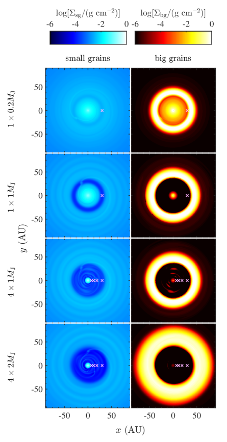
Figure 1.— 2D surface density maps for the small (left column) and big grains (right column) from the hydro simulations (model names labeled on the left). The grey crosses in the convolved images mark the orbits of the planets. The left column is also the scaled surface density distribution of the gas, as we assume that the small grains are well mixed with the gas, $\Sigma_{\rm sg}=0.1\%\times\Sigma_{\rm g}$.

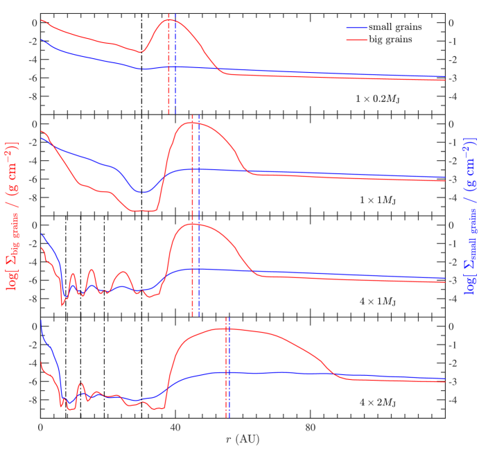
Figure 2.— The azimuthally averaged surface density radial profile for both the small and big grains from the hydro models (model names labeled on the left). Note that the $y$-axis tick mark labels on the left are for the big grains and the ones on the right are for the small grains. The vertical black dash-dot lines indicate the positions of the planets in each model. The vertical blue and red dash-dot lines mark the positions of the peaks in $\Sigma_{\rm sg}$ and $\Sigma_{\rm bg}$ in the outer disk, respectively ($r_{\rm max,out,\Sigma}$ in Table 3). The gap contrast (defined as the ratio of the peak surface density in the outer disk to the floor value inside the gap, $\zeta_{\Sigma}$ in Table 2) is about 1.5 orders of magnitude for the small grains in cases with $M_{\rm p}\geq 1~{}M_{\rm J}$, and $\sim 9$ orders of magnitude for the big grains. Note that $\Sigma_{\rm bg}$ has a hard floor in the hydro simulations, so the gap contrasts for the big grains are lower limits.

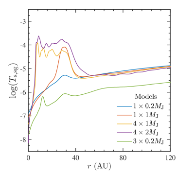
Figure 3.— The dimensionless stopping time $T_{\rm s}$ (Eq. 7) for the small grains (grain size $s$=0.1 $\micron$ as a representative size of the size distribution, Section 2.2). For all models $T_{\rm s,sg}\ll 1$.

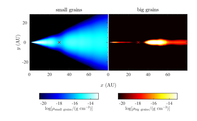
Figure 4.— 2D volume density map for the small (left) and big (right) grains showing the vertical structure ($r-\theta$ plane) at an azimuthal angle $\phi=0^{\circ}$ in Model $1\times 1M_{\rm J}$. The red cross indicates the position of the planet in each panel. The small dust disk is extended in the vertical direction and has a flared structure, while the big grains settle to the disk mid-plane due to aerodynamics effects. The gap around 30 AU is clearly visible in both grains.

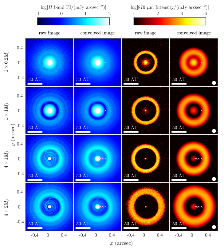
Figure 5.— Raw and convolved $H$ band polarized intensity images (left two columns) and ALMA band 7 (870$~{}\micron$ continuum) intensity images (right two columns) for our models (model names labeled on the left) at face on angle $\theta=0^{\circ}$. Systems are assumed to be at 140 pc. The MCRT images are convolved by a Gaussian kernel with FWHM=0.04$\arcsec$ at $H$ band and FWHM=0.1$\arcsec$ at ALMA band 7 (beam size indicated at the lower right corner in the convolved mm images) to mimic realistic angular resolutions. The grey crosses in the convolved images mark the orbits of the planets. While models with four $M_{\rm p}\geq 1M_{\rm J}$ planets (the bottom two rows) all have a wide gap at both NIR and mm, in Model $1\times 1M_{\rm J}$ (the second row) the NIR gap is much smaller than the mm gap. The NIR gap in Model $1\times 0.2M_{\rm J}$ (the top row) may be to weak to be detectable, while the gap at mm wavelengths is significant.

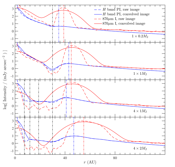
Figure 6.— Azimuthally averaged radial profiles of all images shown in Figure 5. The vertical black dash-dot lines indicate the positions of the planets in each model. The vertical blue and red dash-dot lines mark the positions of the peak intensity in the outer disk in the convolved $H$ band and ALMA images, respectively ($r_{\rm max,out,image}$ in Table 3). In all models, the peak intensity in the outer disk occurs at a larger disk radius at mm than at NIR (more prominent with more massive planets, as in Model $4\times 2M_{\rm J}$). Also, NIR gaps are much shallower than mm gaps, in both raw and convolved images.

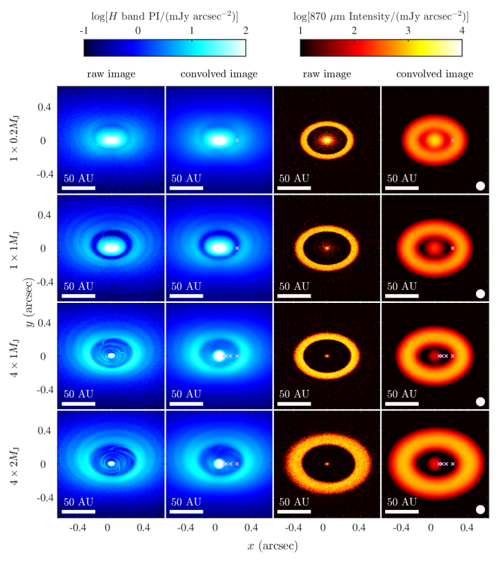
Figure 7.— The same as Figure 5, but for viewing angle $\theta=45^{\circ}$. The lower half in all panels is the front side of the disk.

Figure 8.— Comparison of the $H$ band images at a viewing angle $\theta=45^{\circ}$, between Model $4\times 1M_{\rm J}$ (top row) and Model $4\times 1M_{\rm J}$ with an empty cavity inside 35 AU (bottom row), as discussed in Section 3.3. The red dashed ellipses in the convolved images are fits to the bright ring in the images, and the red crosses mark the position of the star. The material inside the gap cast a shadow in the middle on the far (up) side of the outer gap wall in Model $4\times 1M_{\rm J}$, while the entire outer gap wall is illuminated in Model $4\times 1M_{\rm J}$-empty-gap. As a result of this geometric effect, the ring in the convolved image of Model $4\times 1M_{\rm J}$ appears to be off-center, while in Model $4\times 1M_{\rm J}$-empty-gap the ring is almost on-center.

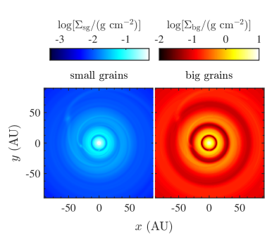
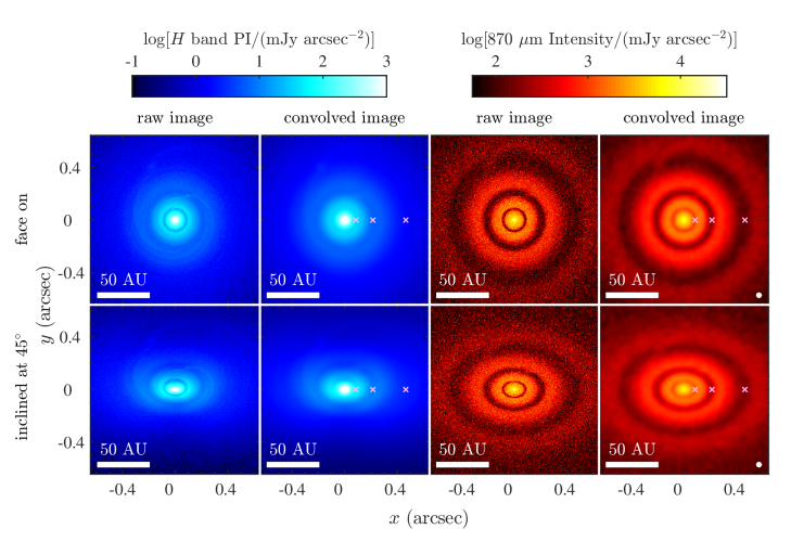
Figure 9.— Model $3\times 0.2M_{\rm J}$: A 0.17 $M_{\odot}$ disk with 3 $0.2M_{\rm J}$ planets located at 12, 30, and 65 AU 0.2 Myr after their formation, showing multiple gaps well separated by rings. Top: 2D surface density map for the small (left) and big (right) grains. The left panel is also the scaled surface density distribution of the gas, as we assume that the small grains are well mixed with the gas, $\Sigma_{\rm sg}=0.1\%\times\Sigma_{\rm g}$. Bottom: Raw and convolved $H$ band polarized intensity images (left two columns) and ALMA band 7 (870$~{}\micron$ continuum) intensity images (right two columns) at face on angle (top row) and an inclined angle $\theta=45^{\circ}$ (bottom row). The grey crosses in the convolved images mark the orbits of the planets. Systems are assumed to be at 140 pc. The convolved images are convolved by a Gaussian kernel with FWHM=0.04$\arcsec$ at $H$ band and FWHM=0.035$\arcsec$ at ALMA band 7 (beam size indicated at the lower right corner in the convolved mm images). The three planets in this case each opens a narrow gap in both the small and big grains. While signals of the gaps in the convolved NIR images are relatively weak, three narrow gaps well separated by bright rings are clearly visible at mm wavelengths at both inclinations. See Section 4.2 for detailed discussion.

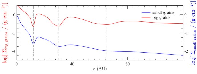
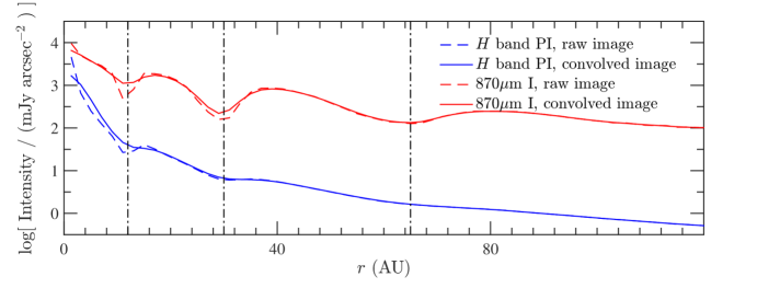
Figure 10.— Radial profiles of the 2D images in Figure 9. Top: The azimuthally averaged surface density radial profile for both the small and big grains from the hydro models. Note that the $y$-axis tick mark labels on the left are for the big grains and the ones on the right are for the small grains. Bottom: Azimuthally averaged radial profiles of all images shown in Figure 5. The vertical black dash-dot lines indicate the positions of the three planets in both panels.

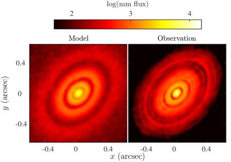
Figure 11.— Comparison between Model $3\times 0.2M_{\rm J}$ with the ALMA observation of HL Tau (1.0 mm, Band 6+7, ALMA Partnership et al. 2015). Model image has an inclination of $45^{\circ}$ and a position angle of $138^{\circ}$. The color scale is logarithmic and the unit is arbitrary.

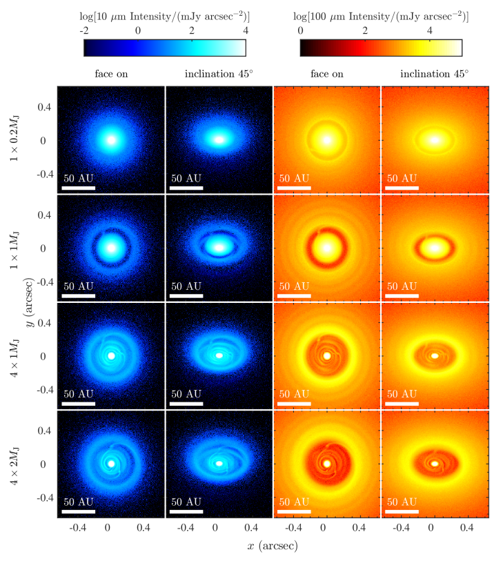
Figure 12.— Raw $10~{}\micron$ intensity images (left two columns) and 100$~{}\micron$ intensity images (right two columns) for our models (model names labeled on the left) at viewing angles $\theta=0^{\circ}$ and $45^{\circ}$. At $10~{}\micron$, gaps appear to be deeper than at $100~{}\micron$, and the shadow casted by the inner disk is visible on the outer gap wall in the inclined disk images.

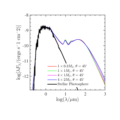
Figure 13.— SEDs for Models $1\times 0.2M_{\rm J}$, $1\times 1M_{\rm J}$, $4\times 1M_{\rm J}$, and $4\times 2M_{\rm J}$ at a viewing angle $\theta=45^{\circ}$. The difference between models is marginal.

References

- Alexander & Armitage (2007) Alexander, R. D., & Armitage, P. J. 2007, MNRAS, 375, 500
- Alexander & Armitage (2009) —. 2009, ApJ, 704, 989
- ALMA Partnership et al. (2015) ALMA Partnership, et al. 2015, ArXiv e-prints
- Andrews et al. (2011) Andrews, S. M., Wilner, D. J., Espaillat, C., Hughes, A. M., Dullemond, C. P., McClure, M. K., Qi, C., & Brown, J. M. 2011, ApJ, 732, 42
- Andrews et al. (2009) Andrews, S. M., Wilner, D. J., Hughes, A. M., Qi, C., & Dullemond, C. P. 2009, ApJ, 700, 1502
- Andrews et al. (2010) —. 2010, ApJ, 723, 1241
- Armitage (2011) Armitage, P. J. 2011, ARA&A, 49, 195
- Artymowicz & Lubow (1994) Artymowicz, P., & Lubow, S. H. 1994, ApJ, 421, 651
- Ataiee et al. (2013) Ataiee, S., Pinilla, P., Zsom, A., Dullemond, C. P., Dominik, C., & Ghanbari, J. 2013, A&A, 553, L3
- Avenhaus et al. (2014) Avenhaus, H., Quanz, S. P., Schmid, H. M., Meyer, M. R., Garufi, A., Wolf, S., & Dominik, C. 2014, ApJ, 781, 87
- Benisty et al. (2015) Benisty, M., et al. 2015, ArXiv e-prints
- Biller et al. (2012) Biller, B., et al. 2012, ApJ, 753, L38
- Birnstiel et al. (2012) Birnstiel, T., Andrews, S. M., & Ercolano, B. 2012, A&A, 544, A79
- Birnstiel et al. (2010) Birnstiel, T., Dullemond, C. P., & Brauer, F. 2010, A&A, 513, A79
- Bohren & Huffman (1983) Bohren, C. F., & Huffman, D. R. 1983, Absorption and scattering of light by small particles
- Brittain et al. (2014) Brittain, S. D., Carr, J. S., Najita, J. R., Quanz, S. P., & Meyer, M. R. 2014, ApJ, 791, 136
- Brown et al. (2009) Brown, J. M., Blake, G. A., Qi, C., Dullemond, C. P., Wilner, D. J., & Williams, J. P. 2009, ApJ, 704, 496
- Bryden et al. (1999) Bryden, G., Chen, X., Lin, D. N. C., Nelson, R. P., & Papaloizou, J. C. B. 1999, ApJ, 514, 344
- Calvet et al. (2005) Calvet, N., et al. 2005, ApJ, 630, L185
- Canovas et al. (2013) Canovas, H., Ménard, F., Hales, A., Jordán, A., Schreiber, M. R., Casassus, S., Gledhill, T. M., & Pinte, C. 2013, A&A, 556, A123
- Casassus et al. (2013) Casassus, S., et al. 2013, Nature, 493, 191
- Close et al. (2014) Close, L. M., et al. 2014, ApJ, 781, L30
- Cuzzi et al. (1993) Cuzzi, J. N., Dobrovolskis, A. R., & Champney, J. M. 1993, Icarus, 106, 102
- D’Alessio et al. (2001) D’Alessio, P., Calvet, N., & Hartmann, L. 2001, ApJ, 553, 321
- D’Angelo et al. (2006) D’Angelo, G., Lubow, S. H., & Bate, M. R. 2006, ApJ, 652, 1698
- de Juan Ovelar et al. (2013) de Juan Ovelar, M., Min, M., Dominik, C., Thalmann, C., Pinilla, P., Benisty, M., & Birnstiel, T. 2013, A&A, 560, A111
- Dodson-Robinson & Salyk (2011) Dodson-Robinson, S. E., & Salyk, C. 2011, ApJ, 738, 131
- Dong et al. (2012a) Dong, R., et al. 2012a, ApJ, 760, 111
- Dong et al. (2012b) —. 2012b, ApJ, 750, 161
- Duffell & MacFadyen (2013) Duffell, P. C., & MacFadyen, A. I. 2013, ApJ, 769, 41
- Dullemond & Dominik (2005) Dullemond, C. P., & Dominik, C. 2005, A&A, 434, 971
- Espaillat et al. (2007) Espaillat, C., Calvet, N., D’Alessio, P., Hernández, J., Qi, C., Hartmann, L., Furlan, E., & Watson, D. M. 2007, ApJ, 670, L135
- Espaillat et al. (2010) Espaillat, C., et al. 2010, ApJ, 717, 441
- Espaillat et al. (2011) Espaillat, C., Furlan, E., D’Alessio, P., Sargent, B., Nagel, E., Calvet, N., Watson, D. M., & Muzerolle, J. 2011, ApJ, 728, 49
- Espaillat et al. (2014) Espaillat, C., et al. 2014, ArXiv e-prints
- Follette et al. (2013) Follette, K. B., et al. 2013, ApJ, 767, 10
- Fouchet et al. (2010) Fouchet, L., Gonzalez, J.-F., & Maddison, S. T. 2010, A&A, 518, A16
- Fu et al. (2014) Fu, W., Li, H., Lubow, S., Li, S., & Liang, E. 2014, ApJ, 795, L39
- Fukagawa et al. (2013) Fukagawa, M., et al. 2013, PASJ, 65, L14
- Fung et al. (2014) Fung, J., Shi, J.-M., & Chiang, E. 2014, ApJ, 782, 88
- Garufi et al. (2013) Garufi, A., et al. 2013, A&A, 560, A105
- Garufi et al. (2014) Garufi, A., Quanz, S. P., Schmid, H. M., Avenhaus, H., Buenzli, E., & Wolf, S. 2014, A&A, 568, A40
- Goldreich & Tremaine (1980) Goldreich, P., & Tremaine, S. 1980, ApJ, 241, 425
- Gonzalez et al. (2012) Gonzalez, J.-F., Pinte, C., Maddison, S. T., Ménard, F., & Fouchet, L. 2012, A&A, 547, A58
- Grady et al. (2013) Grady, C. A., et al. 2013, ApJ, 762, 48
- Guilloteau et al. (2011) Guilloteau, S., Dutrey, A., Piétu, V., & Boehler, Y. 2011, A&A, 529, A105
- Gullbring et al. (1998) Gullbring, E., Hartmann, L., Briceño, C., & Calvet, N. 1998, ApJ, 492, 323
- Hartmann et al. (1998) Hartmann, L., Calvet, N., Gullbring, E., & D’Alessio, P. 1998, ApJ, 495, 385
- Hasegawa & Ida (2013) Hasegawa, Y., & Ida, S. 2013, ApJ, 774, 146
- Hashimoto et al. (2012) Hashimoto, J., et al. 2012, ApJ, 758, L19
- Hashimoto et al. (2011) —. 2011, ApJ, 729, L17
- Henyey & Greenstein (1941) Henyey, L. G., & Greenstein, J. L. 1941, ApJ, 93, 70
- Hinkley et al. (2009) Hinkley, S., et al. 2009, ApJ, 701, 804
- Huélamo et al. (2011) Huélamo, N., Lacour, S., Tuthill, P., Ireland, M., Kraus, A., & Chauvin, G. 2011, A&A, 528, L7
- Hughes et al. (2009) Hughes, A. M., et al. 2009, ApJ, 698, 131
- Isella et al. (2009) Isella, A., Carpenter, J. M., & Sargent, A. I. 2009, ApJ, 701, 260
- Isella et al. (2010) —. 2010, ApJ, 714, 1746
- Jang-Condell (2009) Jang-Condell, H. 2009, ApJ, 700, 820
- Jang-Condell & Boss (2007) Jang-Condell, H., & Boss, A. P. 2007, ApJ, 659, L169
- Jang-Condell & Turner (2012) Jang-Condell, H., & Turner, N. J. 2012, ApJ, 749, 153
- Johansen & Klahr (2005) Johansen, A., & Klahr, H. 2005, ApJ, 634, 1353
- Juhasz et al. (2014) Juhasz, A., Benisty, M., Pohl, A., Dullemond, C., Dominik, C., & Paardekooper, S.-J. 2014, ArXiv e-prints
- Kim et al. (1994) Kim, S.-H., Martin, P. G., & Hendry, P. D. 1994, ApJ, 422, 164
- Kley & Dirksen (2006) Kley, W., & Dirksen, G. 2006, A&A, 447, 369
- Kley & Nelson (2012) Kley, W., & Nelson, R. P. 2012, ARA&A, 50, 211
- Kraus & Ireland (2012) Kraus, A. L., & Ireland, M. J. 2012, ApJ, 745, 5
- Kusakabe et al. (2012) Kusakabe, N., et al. 2012, ApJ, 753, 153
- Kwon et al. (2011) Kwon, W., Looney, L. W., & Mundy, L. G. 2011, ApJ, 741, 3
- Laor & Draine (1993) Laor, A., & Draine, B. T. 1993, ApJ, 402, 441
- Lin & Papaloizou (1993) Lin, D. N. C., & Papaloizou, J. C. B. 1993, in Protostars and Planets III, ed. E. H. Levy & J. I. Lunine, 749–835
- Lucy (1999) Lucy, L. B. 1999, A&A, 344, 282
- Masset (2000) Masset, F. 2000, A&AS, 141, 165
- Mayama et al. (2012) Mayama, S., et al. 2012, ApJ, 760, L26
- Muto et al. (2012) Muto, T., et al. 2012, ApJ, 748, L22
- Nelson & Papaloizou (2003) Nelson, R. P., & Papaloizou, J. C. B. 2003, MNRAS, 339, 993
- Owen (2014) Owen, J. E. 2014, ApJ, 789, 59
- Owen et al. (2012) Owen, J. E., Clarke, C. J., & Ercolano, B. 2012, MNRAS, 422, 1880
- Paardekooper & Mellema (2006) Paardekooper, S.-J., & Mellema, G. 2006, A&A, 453, 1129
- Pérez et al. (2014) Pérez, L. M., Isella, A., Carpenter, J. M., & Chandler, C. J. 2014, ApJ, 783, L13
- Perez et al. (2014) Perez, S., et al. 2014, ArXiv e-prints
- Perrin et al. (2004) Perrin, M. D., Graham, J. R., Kalas, P., Lloyd, J. P., Max, C. E., Gavel, D. T., Pennington, D. M., & Gates, E. L. 2004, Science, 303, 1345
- Pierens & Nelson (2008) Pierens, A., & Nelson, R. P. 2008, A&A, 482, 333
- Piétu et al. (2006) Piétu, V., Dutrey, A., Guilloteau, S., Chapillon, E., & Pety, J. 2006, A&A, 460, L43
- Pinilla et al. (2012a) Pinilla, P., Benisty, M., & Birnstiel, T. 2012a, A&A, 545, A81
- Pinilla et al. (2012b) Pinilla, P., Birnstiel, T., Ricci, L., Dullemond, C. P., Uribe, A. L., Testi, L., & Natta, A. 2012b, A&A, 538, A114
- Pinilla et al. (2014) Pinilla, P., de Juan Ovelar, M., Ataiee, S., Benisty, M., Birnstiel, T., van Dishoeck, E. F., & Min, M. 2014, ArXiv e-prints
- Quanz et al. (2013a) Quanz, S. P., Amara, A., Meyer, M. R., Kenworthy, M. A., Kasper, M., & Girard, J. H. 2013a, ApJ, 766, L1
- Quanz et al. (2013b) Quanz, S. P., Avenhaus, H., Buenzli, E., Garufi, A., Schmid, H. M., & Wolf, S. 2013b, ApJ, 766, L2
- Quanz et al. (2012) Quanz, S. P., Birkmann, S. M., Apai, D., Wolf, S., & Henning, T. 2012, A&A, 538, A92
- Quanz et al. (2011) Quanz, S. P., Schmid, H. M., Geissler, K., Meyer, M. R., Henning, T., Brandner, W., & Wolf, S. 2011, ApJ, 738, 23
- Reggiani et al. (2014) Reggiani, M., et al. 2014, ApJ, 792, L23
- Ricci et al. (2013) Ricci, L., Isella, A., Carpenter, J. M., & Testi, L. 2013, ApJ, 764, L27
- Rice et al. (2006) Rice, W. K. M., Armitage, P. J., Wood, K., & Lodato, G. 2006, MNRAS, 373, 1619
- Rosotti et al. (2013) Rosotti, G. P., Ercolano, B., Owen, J. E., & Armitage, P. J. 2013, MNRAS, 430, 1392
- Ruge et al. (2013) Ruge, J. P., Wolf, S., Uribe, A. L., & Klahr, H. H. 2013, A&A, 549, A97
- Takami et al. (2014) Takami, M., et al. 2014, ApJ, 795, 71
- Takami et al. (2013) —. 2013, ApJ, 772, 145
- Tamura (2009) Tamura, M. 2009, in American Institute of Physics Conference Series, Vol. 1158, American Institute of Physics Conference Series, ed. T. Usuda, M. Tamura, & M. Ishii, 11–16
- Tanii et al. (2012) Tanii, R., et al. 2012, PASJ, 64, 124
- Thalmann et al. (2010) Thalmann, C., et al. 2010, ApJ, 718, L87
- Thalmann et al. (2014) —. 2014, A&A, 566, A51
- Tsukagoshi et al. (2014) Tsukagoshi, T., et al. 2014, ApJ, 783, 90
- van der Marel et al. (2015) van der Marel, N., van Dishoeck, E., Bruderer, S., Perez, L. M., & Isella, A. 2015, ArXiv e-prints
- van der Marel et al. (2013) van der Marel, N., et al. 2013, Science, 340, 1199
- Varnière et al. (2006a) Varnière, P., Bjorkman, J. E., Frank, A., Quillen, A. C., Carciofi, A. C., Whitney, B. A., & Wood, K. 2006a, ApJ, 637, L125
- Varnière et al. (2006b) Varnière, P., Blackman, E. G., Frank, A., & Quillen, A. C. 2006b, ApJ, 640, 1110
- Vorobyov et al. (2014) Vorobyov, E. I., Lin, D. N. C., & Guedel, M. 2014, ArXiv e-prints
- Ward (1997) Ward, W. R. 1997, Icarus, 126, 261
- Weidenschilling (1977) Weidenschilling, S. J. 1977, MNRAS, 180, 57
- Whipple (1972) Whipple, F. L. 1972, in From Plasma to Planet, ed. A. Elvius, 211
- White (1979) White, R. L. 1979, ApJ, 229, 954
- Whitney et al. (2013) Whitney, B. A., Robitaille, T. P., Bjorkman, J. E., Dong, R., Wolff, M. J., Wood, K., & Honor, J. 2013, ApJS, 207, 30
- Whitney et al. (2003a) Whitney, B. A., Wood, K., Bjorkman, J. E., & Cohen, M. 2003a, ApJ, 598, 1079
- Whitney et al. (2003b) Whitney, B. A., Wood, K., Bjorkman, J. E., & Wolff, M. J. 2003b, ApJ, 591, 1049
- Williams & Best (2014) Williams, J. P., & Best, W. M. J. 2014, ApJ, 788, 59
- Williams & Cieza (2011) Williams, J. P., & Cieza, L. A. 2011, ARA&A, 49, 67
- Wolf & D’Angelo (2005) Wolf, S., & D’Angelo, G. 2005, ApJ, 619, 1114
- Youdin & Lithwick (2007) Youdin, A. N., & Lithwick, Y. 2007, Icarus, 192, 588
- Zhang et al. (2014) Zhang, K., Isella, A., Carpenter, J. M., & Blake, G. A. 2014, ApJ, 791, 42
- Zhu et al. (2012) Zhu, Z., Nelson, R. P., Dong, R., Espaillat, C., & Hartmann, L. 2012, ApJ, 755, 6
- Zhu et al. (2011) Zhu, Z., Nelson, R. P., Hartmann, L., Espaillat, C., & Calvet, N. 2011, ApJ, 729, 47
- Zhu & Stone (2014) Zhu, Z., & Stone, J. M. 2014, ApJ, 795, 53
- Zhu et al. (2014) Zhu, Z., Stone, J. M., & Bai, X.-N. 2014, ArXiv e-prints
- Zhu et al. (2013) Zhu, Z., Stone, J. M., & Rafikov, R. R. 2013, ApJ, 768, 143