Decoherence of a solid-state qubit by different noise correlation spectra

Abstract

The interaction between solid-state qubits and their environmental degrees of freedom produces non-unitary effects like decoherence and dissipation. Uncontrolled decoherence is one of the main obstacles that must be overcome in quantum information processing. We study the dynamically decay of coherences in a solid-state qubit by means of the use of a master equation. We analyse the effects induced by thermal Ohmic environments and low-frequency 1/f noise. We focus on the effect of longitudinal and transversal noise on the superconducting qubit’s dynamics. Our results can be used to design experimental future setups when manipulating superconducting qubits.

I Introduction

The scaling-down of microelectronics into the nanometer range will inevitably make quantum effects such as tunnelling and wave propagation important. The use of these quantum devices in gate operations enhances the need of controlling decoherence. Noise from the environment may cause fluctuations in both qubit amplitude and phase, leading to relaxation and decoherence. External perturbations can influence a two-level system in typically two ways: either shifting the individual energy levels (which changes the transition energy and therefore, the qubit’s phase) or inducing energy levels transitions (which changes the level populations). Decoherence is a major hurdle in realising scalable quantum technologies in the solid-state.

Decoherence in qubit systems falls into two general categories. One is an intrinsic decoherence caused by constituents in the qubit system, and the other is an extrinsic decoherence caused by the interaction with uncontrolled degrees of freedom, such as an environment. Understanding the mechanisms of decoherence and achieving long decoherence times is crucial for many fields of science and applications including quantum computation and quantum information nielsen . Most theoretical investigations of how the system is affected by the presence of an environment have been done using a thermal reservoir, usually assuming Markovian statistical properties and defining bath correlations paz ; weiss . However, there has been some growing interest in modelling more realistic environments, sometimes called composite environments, or environments out of thermal equilibrium pra05 ; pra83 ; pra13 .

Lately, there have been many studies focusing in decoherence in a solid-state qubit. The same physical structures that make these superconducting qubits easy to manipulate, measure, and scale are also responsible for coupling the qubit to other electromagnetic degrees of freedom that can be source of decoherence via noise and dissipation. Thus, a detailed mechanism of decoherence and noise due to the coupling of Josephson devices to external noise sources is still required. In Ref.ithier there is a detailed experimental study, inspired from NMR, in order to characterise decoherence in a particular superconducting qubit, known as quantronium. An analysis of different noise sources is presented on the basis of the study of the environmental spectral densities. In paladino authors reviewed the effect of 1/f noise in nano-devices with emphasis on implications for solid-state quantum information. It has been shown that low frequency noise is an important source of decoherence for superconducting qubits. In this detailed review of experimental solid state quantum information, authors dealt with the decoherence effect of $1/f$ noise through a purely dephasing phenomenological approach. In Ref.nesterov , the influence of $1/f$ noise by random dephasing telegraph processes was also modelled, showing that depending on the parameters of the environment, the model can describe both Gaussian and non-Gaussian effects of noise. Ref.zhou presented a phenomenological model for superconducting qubits subject to noise produced by two-state fluctuators whose coupling to the qubit are all roughly the same. In all cases mentioned, authors analysed the qubit’s evolution under pure dephasing conditions, since it is the case where the dynamics can be analytically obtained. When we departure from pure dephasing, i.e., when the noise-system interaction is not longitudinal, no exact analytic solution for the system time evolution is available even for the spin-fluctuator model. In pekola , authors resorted to a master equation approach to study the influence of an environment on a two-level system with an adiabatically changing external field where they have also considered temperature effects. However, authors resorted to a secular approximation for the ground state only, assuming that the excitation rates are exponentially small with respect to the relaxation ones in the quasi-stationary regime. They obtain that in the zero-T limit, the ground state of the system is not affected by the environment and hence, there is no decoherence in that case. This fact can not be true since decoherence at zero temperature does occur. There are simple examples in Literature which demonstrate that decoherence is induced even by a reservoir at zero temperature pla ; pla2 ; pre ; jppdromero . In general, a small system coupled to an environment fluctuates even in the zero-T limit. These fluctuations can take place without generating an energy trace in the bath. The fluctuations in energy of the small system are a peculiar fact of the entanglement with the quantum environment. However, the suppression of the interferences is not as fast as it is at high temperature limit. In the latter case, it is expected to happen, for a quantum Brownian particle of mass $M$, at times of $O(1/2M\gamma_{0}k_{B}TL)$ while it occurs at times bigger than $O(1/\gamma_{0})$ when the environment is at zero temperature pla (where $\gamma_{0}$ is the dissipation constant, $T$ is the environmental temperature, and $L$ the distance between classical trajectories of the particle). In martinis authors study decoherence effects on a superconducting qubit due to bias noise making use of a semiclassical noise model that includes the effect of zero-point and thermal effects.

In the review article by Makhlin et al makhlin , a dephasing model is considered in which the spin-system is coupled to an Ohmic environment at thermal equilibrium. They show that the dephasing time is shorter than the measurement time, and they estimate the mixing time, i. e. the time scale on which transitions induced by the measurement occur. They analyse the dephasing rate in an exactly solvable limit of a qubit with no tunnelling term.

In berger , noise is described by fluctuations in the effective magnetic field which are directed either in the $z$ axis -longitudinal noise- or in a transverse direction -transversal noise. Both types of noise have been phenomenologically modelled by making different assumptions on these fluctuations, such as being due to a stationary, Gaussian and Markovian process. The results obtained were applied on adiabatic geometric phase. They experimentally study which noise -either radial or angular- contribute to the geometric (Berry) and dynamical phase, observing that the radial noise is more destructive.

In this context, we aim to gather the main of these features (and the ones that have been neglected by the sake of simplicity) that have been studied separately in a single approach by the study of decoherence process from a master equation for a superconducting qubit. By considering a general approach of the qubit and environment, we include different channels of decoherence (purely dephasing and decoherence by anomalous diffusion coefficients). This approach does not admit an analytical solution in the end but by means of a numerical solution of the reduced density matrix we can obtain the dynamics of the qubit. This allows to focus on different noise sources and different couplings to the environment and gives a common framework to study the decoherence process of the qubit. This is particularly important in the case of very low temperature fluctuations, which sometimes are considered to be harmless to the unitary evolution of the qubit. In such a complete case, the evolution of the system undergoes dephasing and relaxation leading to serious problems in maintaining the quantum state.

In this article, we shall present a fully quantum open-system approach to analyse the non-unitary dynamics of the solid-state qubit when it evolves under the influence of external fluctuations. We consider the qubit coupled in longitudinal and transversal directions, that is a model where populations and coherences are modified by the environment. We study the dynamics and decoherence-induced process on the superconducting qubit. The paper is organised as follows: In Sec. II, we develop a general quantum open-system model in order to consider different types of fluctuations (longitudinal and/or transverse) that induce decoherence on the main system. In Sec. III we present the master equation approach for a general coupling of a superconducting, and numerically compute the non-unitary evolution characterised by fluctuations, dissipation, and decoherence. This gives us a complete insight into the state of the system: complete knowledge of different dynamical time scales and analysis of the effective role of noise sources inducing diffusion and dissipation. We also analyse low-frequency $1/f$ noise as coming from a fluctuator environment, by defining the corresponding spectral density. The comprehension of the decoherence and dissipative processes should allow their further suppression in future qubits designs or experimental setups. In Sec. IV, we analyse the effect induced in the system by thermal Ohmic environments, through a non-purely dephasing process, including the case of a zero-temperature bath. In Sec.V we study the decoherence induced by a $1/f$ noise. In both cases, we particularly study the difference between the longitudinal and transversal couplings and provide analytical estimations of decoherence time when possible. Finally in Sec. VI, we summarise our final remarks.

II Model for a solid-state qubit

Superconducting qubits are made of inductors, capacitors, and Josephson junctions (JJ) Josephson , where a JJ consists of a thin layer of insulator between superconducting electrodes. A quantum circuit consisting only of inductors and capacitors gives rise to parabolic energy potentials exhibiting equally spaced energy levels, which are not practical for qubits. The JJ provides the necessary nonlinearity to the system, leading to non-parabolic energy potentials with unequally spaced energy levels such that two out of several energy levels, serving as the qubit states $|0\rangle$ and $|1\rangle$, can be isolated. Experimental observation of Rabi oscillations in driven quantum circuits have shown several periods of coherent oscillations, confirming the validity of the two-level approximation and possibility of coherently superimpose the computational two states of the system. Nevertheless, the unavoidable coupling to a dissipative environment surrounding the circuit represents a source of relaxation and decoherence that limits the performances of the qubit for quantum computation tasks. Therefore, for the implementation of superconducting circuits as quantum bits, it is necessary to understand the way the system interacts with the environmental degrees of freedom, and to reduce their effect, if possible.

When the two lowest energy levels of a current biased Josephson junction are used as a qubit, the qubit state can be fully manipulated with low and microwave frequency control currents. Circuits presently being explored combine in variable ratios the Josephson effect and single Cooper-pair charging effects. In all cases the Hamiltonian of the system can be written as, $H=\frac{\hbar}{2}\omega_{a}\sigma_{z}+\hbar\Omega_{\rm R}\cos(\omega t+\varphi_{\rm R})\sigma_{x}$, where $\hbar\Omega_{\rm R}$ is the dipole interaction amplitude between the qubit and the microwave field of frequency $\omega$ and phase $\varphi_{\rm R}$. $\Omega_{\rm R}/2\pi$ is the Rabi frequency. This Hamiltonian can be transformed to a rotating frame at the frequency $\omega$ by means of an unitary transformation defined by the operator $U=\exp{(i\omega t\sigma_{z}/2)}$ leek and, after the rotating wave approximation (ignoring terms oscillating at $2\omega$), resulting in a new effective Hamiltonian of the form

$$H_{\text{eff}}=\frac{\hbar}{2}\left(\Delta\sigma_{z}+\Omega_{x}\sigma_{x}+\Omega_{y}\sigma_{y}\right),$$ (1)

where $\Omega_{x}=\Omega_{\rm R}\cos\varphi_{\rm R}$ and $\Omega_{y}=\Omega_{\rm R}\sin\varphi_{\rm R}$. Then, we shall consider the dynamics of a generic two-level system steered by a system’s Hamiltonian of the type (where we have set $\hbar=1$ all along the paper)

$$H_{\text{Total}}=H_{\text{eff}}+H_{\rm int}+H_{\cal E},$$ (2)

where $H_{\cal E}$ is the Hamiltonian of the bath. The interaction Hamiltonian (in the rotating frame) is thought as some longitudinal and transverse noise coupled to the main system:

$$H_{\rm int}=\frac{1}{2}\left({\hat{\delta\omega_{1}}}\sigma_{x}+{\hat{\delta\omega_{2}}}\sigma_{y}+{\hat{\delta\omega_{0}}}\sigma_{z}\right).$$ (3)

By considering this interaction Hamiltonian we are implying that the superconducting qubit is coupled to the environment by a coupling constant in the $\hat{z}$ direction, called longitudinal direction, affecting only the coherences; and a coupling in the transverse directions ($\hat{x}$ and $\hat{y}$), which modify populations and coherences in a different rate. This type of coupling is a generalisation of the bidirectional coupling recently used in pra89 to compute the geometric phase of a superconducting qubit. It is important to note that the derivation of a master equation has not been done before for a solid-state qubit.

III Master equation approach

We derive a master equation for general noise terms ${\hat{\delta\omega_{1}}}$, ${\hat{\delta\omega_{2}}}$ and ${\hat{\delta\omega_{0}}}$. We consider a weak coupling between system and environment and the bath sufficiently large to stay in a stationary state. In other words, the total state $\rho_{\cal SE}$ (system and environment) can be split as $\rho_{\cal SE}\approx\rho(t)\times\rho_{\cal E}$, for all times. It is important to stress that due to the Markov regime, we restrict to cases for which the self-correlation functions generated at the environment (due to the coupling interaction) would decay faster than typical variation scales in the system breuer . In the interaction picture, the evolution of the total state is ruled by the Liouville equation

$${\dot{\rho}}_{\cal SE}=-i\left[H_{\rm int},\rho_{\cal SE}\right],$$ (4)

where we have denoted the state $\rho_{\cal SE}$ in the interaction picture in the same way than before, just in order to simplify notation. A formal solution of the Liouville equation can be obtained perturbatively using the Dyson expansion.

From this expansion, one can obtain a perturbative master equation, up to second order in the coupling constant between system and environment for the reduced density matrix $\rho={\mbox{T}r}_{\cal E}\rho_{\cal SE}$. In the interaction picture the formal solution reads as

$$\rho(t)\approx\rho(0)-i\int_{0}^{t}ds{\mbox{T}r}_{\cal E}\left(\left[H_{\rm int}(s),\rho_{\cal SE}(0)\right]\right)-\int_{0}^{t}ds_{1}\int_{0}^{s_{1}}ds_{2}{\mbox{T}r}_{\cal E}\left(\left[H_{\rm int}(s),\left[H_{\rm int}(t),\rho_{\cal SE}(0)\right]\right]\right).$$

In order to obtain the full master equation for the qubit, it is necessary to perform the temporal derivative of the previous equation and assume that the system and the environment are not initially correlated. In addition, we consider that the ${\hat{\delta\omega_{i}}}$ of the $H_{\rm int}$ (Eq.(3)) are operators acting only on the Hilbert space of the environment (and the Pauli matrices applied on the system Hilbert space). Finally, the master equation explicitly reads,

$$\dot{\rho} = -i\left[H_{\rm eff},\rho\right]-d_{xx}(t)\left[\sigma_{x},\left[\sigma_{x},\rho\right]\right]-f_{xy}(t)\left[\sigma_{x},\left[\sigma_{y},\rho\right]\right]-f_{xz}(t)\left[\sigma_{x},\left[\sigma_{z},\rho\right]\right]$$

$$- f_{zx}(t)\left[\sigma_{z},\left[\sigma_{x},\rho\right]\right]-f_{yx}(t)\left[\sigma_{y},\left[\sigma_{x},\rho\right]\right]-d_{yy}(t)\left[\sigma_{y},\left[\sigma_{y},\rho\right]\right]-f_{yz}(t)\left[\sigma_{y},\left[\sigma_{z},\rho\right]\right]$$

$$- f_{zy}(t)\left[\sigma_{z},\left[\sigma_{y},\rho\right]\right]-d_{zz}(t)\left[\sigma_{z},\left[\sigma_{z},\rho\right]\right]+i\gamma_{xy}\left[\sigma_{x},\left\{\sigma_{y},\rho\right\}\right]+i\gamma_{xz}\left[\sigma_{x},\left\{\sigma_{z},\rho\right\}\right]+i\gamma_{zx}\left[\sigma_{z},\left\{\sigma_{x},\rho\right\}\right]$$

$$+ i\gamma_{zy}\left[\sigma_{z},\left\{\sigma_{y},\rho\right\}\right]+i\gamma_{yx}\left[\sigma_{y},\left\{\sigma_{x},\rho\right\}\right]+i\gamma_{yz}\left[\sigma_{y},\left\{\sigma_{z},\rho\right\}\right],$$

where the noise effects are included as the normal ($d_{xx}$, $d_{yy}$ and $d_{zz}$) and anomalous diffusion coefficients ($f_{ij}$ with $i,j=x,y,z$). The dissipative effects are considered in the corresponding coefficients ($\gamma_{ij}$ with $i,j=x,y,z$). Thus, Eq.(III) considers both diffusion and dissipation effects for a superconducting qubit with couplings as in Eq.(3),

$$d_{xx}(t) = \int_{0}^{t}ds\,\nu_{1}(s)\,X_{1}(-s),~{}~{}~{}d_{yy}(t)=\int_{0}^{t}ds\,\nu_{2}(s)\,Y_{2}(-s),~{}~{}~{}d_{zz}(t)=\int_{0}^{t}ds\,\nu_{0}(s)\,Z_{0}(-s),$$

$$f_{xy}(t) = \int_{0}^{t}ds\,\nu_{1}(s)\,Y_{1}(-s),~{}~{}~{}f_{xz}(t)=\int_{0}^{t}ds\,\nu_{1}(s)\,Z_{1}(-s),~{}~{}~{}f_{zx}(t)=\int_{0}^{t}ds\,\nu_{0}(s)\,X_{0}(-s),$$

$$f_{zy}(t) = \int_{0}^{t}ds\,\nu_{0}(s)\,Y_{0}(-s),~{}~{}~{}f_{yx}(t)=\int_{0}^{t}ds\,\nu_{2}(s)\,X_{2}(-s),~{}~{}~{}f_{yz}(t)=\int_{0}^{t}ds\,\nu_{2}(s)\,Z_{2}(-s)$$ (6)

$$\gamma_{xy}(t) = \int_{0}^{t}ds\,\eta_{1}(s)\,Y_{1}(-s),~{}~{}~{}\gamma_{xz}(t)=\int_{0}^{t}ds\,\eta_{1}(s)\,Z_{1}(-s),~{}~{}~{}\gamma_{yx}(t)=\int_{0}^{t}ds\,\eta_{2}(s)\,X_{2}(-s),$$

$$\gamma_{zx}(t) = \int_{0}^{t}ds\,\eta_{0}(s)\,X_{0}(-s),~{}~{}~{}\gamma_{yz}(t)=\int_{0}^{t}ds\,\eta_{2}(s)\,Z_{2}(-s),~{}~{}~{}{\mathrm{and}}~{}~{}~{}\gamma_{zy}(t)=\int_{0}^{t}ds\,\eta_{0}(s)\,Y_{0}(-s).$$

These coefficients are defined in terms of the noise and dissipation kernels, $\nu(t)$ and $\eta(t)$, respectively. These kernels are generally defined, for unspecified operators ${\hat{\delta\omega_{0}}}(t)$, ${\hat{\delta\omega_{1}}}(t)$ and ${\hat{\delta\omega_{2}}}(t)$, as

$$\nu_{a}(t)=\frac{1}{2}\langle\left\{{\hat{\delta\omega_{a}}}(t),{\hat{\delta\omega_{a}}}(0)\right\}\rangle,$$ (7)

$$\eta_{a}(t)=\frac{1}{2}\langle\left[{\hat{\delta\omega_{a}}}(t),{\hat{\delta\omega_{a}}}(0)\right]\rangle,$$ (8)

with $a=1,2,0$. The functions $X_{a},Y_{a}$, and $Z_{a}$ appearing in Eq.(6) are given in the Appendix. It is easy to check that if the Rabi frequency is zero and $\delta\hat{\omega}_{1}=0=\delta\hat{\omega}_{2}$, we recover the dynamics of a spin-$1/2$ precessing a biased field Bloch vector ${\bf R}$.

The intention is to study environmental-induced decoherence by means of the use of the master equation. We will mainly concentrate on two types of external noise sources. On one side, we shall consider that the environment is characterised by an Ohmic spectral density, as the one commonly used in models of Quantum Brownian Motion (QBM) or in the well known spin-boson model leggett ; pra . In these examples, the environment is represented by an infinite set of harmonic oscillators at thermal equilibrium. On the other side, we shall analyse decoherence induced effects coming from spin-environments, for example spin-fluctuator models, that give us the possibility to study $1/f$ noise-effects via the master equation approach, without resorting to classical statistical evolutions or phenomenological models. Once the coefficients in Eqs.(6) are defined by the use of the corresponding spectral correlations Eqs.(7) and (8), we can numerically solve the master equation and obtain the evolution in time of the reduced density matrix.

IV Ohmic environment

A relevant contribution to decoherence in solid-state qubits, is introduced by the electromagnetic noise of the control circuit, typically Ohmic noise at low frequencies. In this Section, we model this kind of environments by means of an infinite set of harmonic oscillators with an Ohmic spectral density. An environment composed by harmonic oscillators at thermal equilibrium at temperature T is commonly introduced in order to take into account dissipative effects, additionally to noise or fluctuations effects.

It is easy to see that in the case that the environment is modelled by a set of harmonic oscillators, the noise (Eq. (7)) and dissipation (Eq.(8)) kernels become

$$\nu_{a}(t)=\frac{1}{2}\sum_{n}\lambda_{a,n}^{2}\langle\left\{q_{n}(t),q_{n}(0)\right\}\rangle,$$ (9)

$$\eta_{a}(t)=\frac{1}{2}\sum_{n}\lambda_{a,n}^{2}\langle\left[q_{n}(t),q_{n}(0)\right]\rangle,$$ (10)

where $q_{n}$ are the position operators for the environmental degrees of freedom.

The noise correlations can be defined by their spectral density $J_{a}(\omega)=1/(2\pi)\int dte^{i\omega t}\langle{\hat{\delta\omega_{a}}}(0){\hat{\delta\omega_{a}}}(-s)\rangle_{\cal E}$ with $a=0,1,2$. If we assume the environment is composed by an infinite set of harmonic oscillators, it is useful to use the relation

$$\sum_{n}^{N}\frac{\lambda_{n}^{2}}{2m_{n}\omega_{n}}f(\omega_{n})=\int_{0}^{\infty}J(\omega)f(\omega)d\omega,$$ (11)

in order to express kernels in terms of integrals in frequency. For example, using Eqs. (9) and (10), the noise and dissipation kernels can be written as

$$\nu_{a}(t) = \int_{0}^{\infty}J_{a}(\omega)\cos(\omega t)\coth(\frac{\beta\omega}{2})d\omega,$$ (12)

$$\eta_{a}(t) = \int_{0}^{\infty}J_{a}(\omega)\sin(\omega t)d\omega,$$ (13)

where $\beta=1/k_{B}T$ is the equilibrium temperature of the environment.

In this model, we use $J_{a}(\omega)=\gamma_{a}\omega\exp[-\omega/\Lambda]$ as the spectral density of the environment. This definition allows to calculate the noise and dissipation kernels from Eqs.(12) and (13) pra . In the definition of $J(\omega)$, $\Lambda$ is a physical ultraviolet cutoff, which represents the biggest frequency present in the environment.

Starting with an arbitrary initial superposition state in the Bloch sphere, $|\psi\rangle=\cos(\theta/2)|0\rangle+\sin(\theta/2)|1\rangle$, we numerically solve the master equation at different environmental temperatures. In the high temperature limit, one can expand the $\coth(\beta\omega/2)$ for small $\beta$, and obtain the noise kernel (the one that depends on temperature) as $\nu_{a}(t)=\gamma_{a}k_{B}T\delta(t)$ (where, with the sub-index $a=0$ we denote the longitudinal coupling and with the sub-index $a=1,2$ transversal noise). In this limit, it is trivial to evaluate the diffusion terms in Eq.(6), to obtain that $d_{xx}=\gamma_{1}k_{B}T$, $d_{yy}=\gamma_{2}k_{B}T$, $d_{zz}=\gamma_{0}k_{B}T$, and all $f_{ij}=0$ (there is no anomalous diffusion terms). In the opposite case, when $T\rightarrow 0$, the diffusion kernel yields $\nu_{a}(t)=\gamma_{a}(t\Lambda\sin(\Lambda t)+\cos(\Lambda t)-1)/t^{2}$. With this kernel all the diffusion coefficients in Eq.(6) can be obtained for a zero-T environment. It is important to remark that they are all different from zero and contribute to the master equation. We do not present here the explicit expression of them since their form is not relevant. The dissipative coefficients for the Ohmic environment, can be all calculated from the dissipation kernel Eq.(13). Thus, these kernels are given by $\eta_{a}(t)=\gamma_{a}\delta^{\prime}(t)$, which are independent on temperature. Therefore, dissipation coefficients (in Eq.(6)) are $\gamma_{xy}=2\Delta\gamma_{1}$, $\gamma_{xz}=-2\gamma_{1}\Omega_{y}$, $\gamma_{zx}=2\gamma_{0}\Omega_{y}$, $\gamma_{zy}=-2\Omega_{x}\gamma_{0}$, $\gamma_{yx}=-2\gamma_{2}\Delta$, and $\gamma_{yz}=2\gamma_{2}\Omega_{x}$.

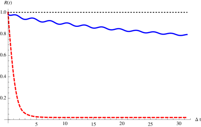
Figure 1: (Color online) Temporal evolution of the absolute value of the Bloch vector for different environments coupled to the superconducting qubit. The black dotted line is the unitary evolution, i.e. no noise present in the evolution. The red dashed line represents an Ohmic environment in the high temperature limit while the blue solid line represents an Ohmic environment at zero temperature. It is easy to note that the state vector of the system is more affected by the influence of the high temperature environment. However, we must note that the initially pure state loses purity even at zero temperature for the same values of $\gamma_{a}$. We have considered the effect of longitudinal and transverse noise simultaneously. Parameters used: $\Omega_{\rm R}=0.1\Delta,~{}\gamma_{0}=0.002=\gamma_{1},~{}\Lambda=100\Delta,~{}T=100\Delta$. We have set $\varphi_{\rm R}=0$ and $\gamma_{2}=0$ for simplicity. The initial state is given by $\theta=2/3\pi$ .

In Fig.1 we present the absolute value of the Bloch vector of the state system $\bf{R}$ as a function of time for more than one period $\tau=2\pi/\tilde{\Omega}$, with $\tilde{\Omega}=\Delta^{2}/\sqrt{\Delta^{2}+\Omega_{R}^{2}}$. Qualitatively, decoherence can be thought as the deviation of probabilities measurements from the ideal intended outcome. Therefore, decoherence can be understood as fluctuations in the Bloch vector ${\bf R}$ induced by noise. Since decoherence rate depends on the state of the qubit, we will use as a measure of decoherence the change in time of the absolute value of ${\bf R}$, starting from $|{\bf R}|=1$ for the initial pure state, and decreasing as long as the quantum state losses purity. In Fig.1, the black dotted line is the unitary evolution (as expected ${\mathbf{R}}=1$ for all times), while the red dashed line is the evolution of the Bloch vector of a qubit evolving under a high temperature Ohmic environment. This kind of environment is very destructive and the state vector is soon removed from the surface of the sphere (where purity states lie). The blue solid line represents the behaviour of the Bloch vector when the qubit is evolving under the influence of a zero temperature Ohmic environment. It is easy to note that the state losses purity even at zero temperature, though the influence of the environment is not as drastic as when the temperature is high. We have considered the effect of the longitudinal and transverse noise simultaneously. These facts can also be seen in Fig.2, where we plot the trajectories in the Bloch sphere. It is easy to see, that the Ohmic environment at high temperature (red solid line) is very drastic, removing the state from the Bloch sphere surface in a very short timescale. The qubit under the presence of an Ohmic environment at zero temperature (black dashed line) looses purity as well, but the timescale at which the quantum coherences are removed takes longer.

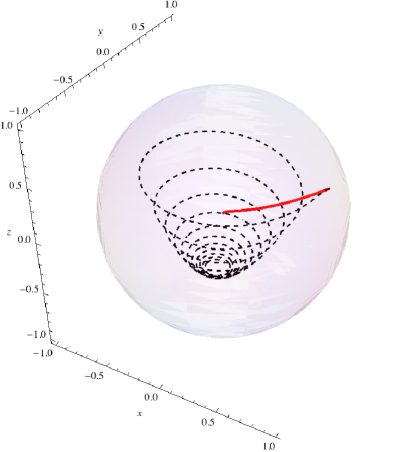
Figure 2: (Color online). We present the trajectories of the qubit in the Bloch sphere for two periods of time. The black dashed line is the evolution for a qubit in the presence of an Ohmic environment at zero temperature. The red solid line is for an Ohmic environment at high temperature. We have considered the effect of longitudinal and transverse noise simultaneously. Parameters used: $\Omega_{\rm R}=0.1\Delta,~{}\gamma_{0}=0.002=\gamma_{1},~{}\Lambda=100\Delta,~{}T=100\Delta$. We have set $\varphi_{\rm R}=0$ and $\gamma_{2}=0$ for simplicity. The initial state is given by $\theta=2/3\pi$.

When we deal with a master equation of the form of Eq.(III), it is known that all real terms contribute to diffusion effects while imaginary ones to renormalisation and dissipation pla . As decoherence is the dynamical suppression of the quantum coherences, the off-diagonal elements of the reduced density matrix are also a good measure of how the environment affects the dynamics of the qubit. For a general process (non-purely dephasing process), the reduced density matrix can be represented as

$$\rho_{\rm r}(t) = \bigg{(}\begin{array}[]{cc}a_{00}(t)&a_{01}{\cal F}(t)\\ a_{10}{\cal F}(t)^{*}&a_{11}(t)\end{array}\bigg{)},$$ (16)

where ${\cal F}(t)$ can be related to the decoherence factor (which is responsible for the exponential decay of the coherences). In the case of a longitudinal coupling only, the populations remain constant and ${\cal F}(t)$ is the decoherence factor defined as $e^{-\int d_{zz}(t^{\prime})dt^{\prime}}$, where $d_{zz}(t)$ is the diffusion coefficient. Independently of its formal expression, we know that ${\cal F}(t)$ must be a decaying function by which after some time bigger than the decoherence time $t>t_{D}$, the quantum coherences of the density matrix can be neglected. In the case of a more general coupling such as the one studied here, the decoherence factor is composed by the diffusion coefficient ($d_{zz}(t)$, i.e. in this case) and some other anomalous diffusion and dissipation coefficients such as $f_{zx}(t)$ and $\gamma_{zy}(t)$, that affect the off-diagonal terms with no defined sign.

Due to the fact that we are considering a general qubit (such as $H_{\rm eff}$ in Eq. (1)) and a general coupling ($H_{\rm{int}}$ in Eq. (3)), there are some more coefficients that contribute to dissipation process such as $d_{xx}(t)$, $f_{xz}(t)$, $f_{xy}(t)$, $f_{zy}(t)$ and $\gamma_{xy}(t)$ Benenti . These complete set of coefficients provide a very complicated dynamics that only can only be solved numerically.

In order to study the decoherence process suffered by the qubit we propose also the study of the off-diagonal terms as well as the absolute value of the Bloch vector. The difference between both quantities is that while the latter one provides information about the purity of the state, the former gives information about the decoherence timescale ($t_{D}$), i.e. the time after which the coherences of the reduced density matrix can be neglected. Therefore, we shall look at the behaviour of the quantum coherences, i.e the off-diagonal terms of the reduced density matrix $\rho_{r_{\textrm{off}}}(t)$ to study the influence of the environment on the system’s evolution and derive, when possible, a decoherence timescale.

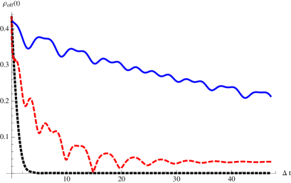
Figure 3: (Color online) Temporal evolution of the absolute value of the quantum coherence (denoted as $\rho_{r_{\textrm{off}}}(t)$), namely the off-diagonal terms of the qubit system ($\rho_{01}(t)$). The black dotted line is the evolution of the coherences in the case the qubit is coupled to a high-T environment ($\gamma_{0}=\gamma_{1}=0.02$ and $T/\Delta=100$). In this case, the system losses coherence quickly and with no possibility of re-coherence. The red dashed line, shows the evolution of the coherence in the limit of zero environmental temperature (with cutoff in frequencies $\Lambda=100\Delta$ and $\gamma_{0}=\gamma_{1}=0.02$). Finally, the blue solid oscillatory line represents the evolution of the coherence for a smaller value of $\gamma_{a}$ at zero temperature ($\gamma_{0}=\gamma_{1}=0.002$). We have considered the effect of longitudinal and transverse noise simultaneously. It is easy to see that the system also losses coherence when the environment is at zero temperature. The final value of the off-diagonal term differs from the one in the high-T case, due to the presence of diffusion and other dissipative coefficients in the master equation. We have considered $\Omega_{\rm R}=0.1\Delta$, $\gamma_{2}=0$, $\varphi_{\rm R}=0$, and the initial state is given by $\theta=2/3\pi$.

In Fig.3 we present the evolution in time of the off-diagonal terms of the qubit’s reduced density matrix ($\rho_{r_{\textrm{off}}}(t)$) as a function of dimensionless time ($\Delta t$), in the case of high and zero temperature and for different dissipation constants in the weak coupling limit. The black dotted line is the solution of the master equation in the limit of high temperature (for dimensionless parameter $T/\Delta=100$). As expected, off-diagonal terms in the reduced density matrix decay quickly to their minimum value, reaching a steady state of minimum coherence. A relevant result is the one obtained in the limit of $T=0$ environmental temperature represented by the blue solid line $\gamma_{a}=0.002$ and the red dashed one $\gamma_{a}=0.02$. In this cases, we can see that, the coherences in the system decay (more slowly than in the case of high temperature) with time, reaching an asymptotic value of minimum coherence, at a timescale different from the one corresponding to the high-T limit. The smaller the value of the coupling, the longer it takes the system to reach the asymptotic value. This is mainly due to the presence, in the master equation for T = 0, of anomalous diffusion coefficients, which are absent in the case of high-T. Nevertheless, we show that fluctuations at zero-T also induce decoherence in the solid-state qubit, with a lower efficiency than in the thermal case, but strong enough to destroy the unitary evolution.

In order to have a rough analytical estimation of decoherence times, we consider that the qubit is solely coupled in the longitudinal direction, and that there are no anomalous and dissipation terms in the master equation. This means that for the moment we neglect the effect of the tunnelling term (proportional to both transverse directions) in the main system Hamiltonian. Thus, we may follow the result given in Refs. pla ; pra for the purely dephasing model. There, decoherence time in the high temperature approximation can be estimated as $t_{D}\sim 2/(k_{B}T\gamma_{0})$ makhlin , which does not depend on the frequency cutoff $\Lambda$. Considering parameters used in Fig. 3, one can estimate decoherence time to be $t_{D}\sim 1\Delta$, in good agreement with the corresponding plots in Fig. 3. For the Ohmic case at zero temperature, the decoherence scales as $t_{D}\geq 2/(\gamma_{0}\Lambda\pi)$ for times $\Lambda t\geq 1$. In this case, decoherence is delayed as $\gamma_{0}$ decreases. This is a very long bound for decoherence time, especially when the longitudinal coupling constant is very small. Indeed, this reflects the fact that the contribution of all the coefficients in the master equation (anomalous diffusion and dissipation coefficients) are important in the limit of zero temperature, as can be seen in Fig. 3.

Figure 4: (Color online) Temporal evolution of the coherence ($\rho_{r_{\textrm{off}}}(t)$) (its absolute value) of the qubit system coupled to a high temperature Ohmic environment. The red dashed line represent the evolution of the coherence when the qubit is coupled only in the transverse direction, namely through $\delta\omega_{1}$. In this case, we use $\gamma_{1}=0.02$ and $\gamma_{0}=0$. The black dotted line is the evolution of the coherences in the case the qubit is coupled to a high-T environment only in the longitudinal direction, i.e. through $\delta\omega_{0}$. This means $\gamma_{1}=0$ and for example, $\gamma_{0}=0.02$. Finally, the blue solid line (almost coincides with the black dotted line) is the evolution of the coherence when the qubit is equally coupled in both directions, i.e. $\gamma_{0}=0.02$ and $\gamma_{1}=0.02$. We have considered $\Omega_{\rm R}=0.1\Delta$, $\varphi_{\rm R}=0$, $\gamma_{2}=0$, and $T=100\Delta$. The initial state is given by $\theta=\pi/3$.

As we are considering a bidirectional coupling in our model, it is interesting to see if there is a direction in which noise becomes more important. As the value of $\gamma_{0}$ and $\gamma_{1}$ imply the coupling with the environment, we can turn off one of the couplings to study the effect of noise in the longitudinal and transverse directions. Thus, we consider only one transverse direction to make this analysis, by setting $\gamma_{2}=0$, since we consider the difference between longitudinal and transverse (either one) couplings. In Fig.4 we follow the decay of the quantum coherences of the reduced density matrix corresponding to each of the cases considered: only longitudinal coupling, only transversal coupling and both couplings. The red dashed line represents the evolution of the coherence when the qubit is coupled only in the transverse direction, namely through $\delta\omega_{1}$. In this case, we use $\gamma_{1}=0.02$ and $\gamma_{0}=0$. The black dotted line is the evolution of the coherences in the case the qubit is coupled to a high-T environment only in the longitudinal direction, i.e. through $\delta\omega_{0}$. This means $\gamma_{1}=0$ and for example, $\gamma_{0}=0.02$. Finally, the blue solid line (which falls together with the black dotted line) is the evolution of the coherence when the qubit is equally coupled in both directions, i.e. $\gamma_{0}=0.02$ and $\gamma_{1}=0.02$. It is easy to see that decoherence is mainly ruled by the longitudinal direction ($t_{D}\sim 1\Delta$) which means that noise in the $\hat{z}$-direction affects more the unitary dynamics of the system than noise in $\hat{x}$ direction.

We can also study the leading behaviour (related to the coupling of the system) for a zero-T Ohmic environment. In Fig.5 we show the behaviour of the quantum coherences ($\rho_{r_{\textrm{off}}}(t)$) for different couplings. The black dotted line is a bidirectional (longitudinal and transverse) coupling of same value $\gamma_{a}=0.02$. The red dashed line is for a transverse coupling, i.e. $\gamma_{1}=0.02$ and $\gamma_{0}=0$. Finally, the blue solid line is only a longitudinal coupling $\gamma_{0}=0.02$ and $\gamma_{1}=0$. We can note the longer decoherence timescale in comparison to an Ohmic environment in the high temperature limit, see for example Fig.4. It is also important to remark that at zero temperature, all noises are equally important. This is a quiet important observation. By taking a thorough look, at shorter times, we can see that the blue solid line decays faster, corresponding to a longitudinal coupling. However, the timescale at which the longitudinal coupling decays is comparable to the timescale of a transversal coupling (in magnitude order). However, the intrinsic dynamics of the system delays the reaching of the asymptotic limit, since we are studying the weak coupling limit.

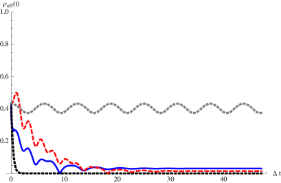
Figure 5: (Color online) Temporal evolution of the absolute value of the coherence ($\rho_{r_{\textrm{off}}}(t)$) of the qubit system coupled to a zero-T Ohmic environment. The red dashed line is the evolution of the coherences in the case the qubit is coupled only in the transverse direction, i.e. through $\delta\omega_{1}$. This means $\gamma_{0}=0$ and for example, $\gamma_{1}=0.02$. The black dotted line represents the evolution of the coherence when the qubit is equally coupled in both directions, i.e. $\gamma_{0}=0.02$ and $\gamma_{1}=0.02$. Finally, the blue solid line is the evolution of the coherence when the qubit is coupled only in the longitudinal direction, namely through $\delta\omega_{0}$. In this case, we use $\gamma_{0}=0.02$ and $\gamma_{1}=0$. We have also included in a grey dotted line the oscillatory unitary behaviour of the coherence. We have considered $\Omega_{\rm R}=0.1\Delta$, $\varphi_{\rm R}=0$, $\gamma_{2}=0$, and the initial state is given by $\theta=\pi/3$.

V 1/f noise

Much effort has been spent recently to understand how noise at low frequencies affects the dynamics of superconducting qubits, both from a theoretical and experimental point of view. In solid-state systems decoherence is potentially strong due to numerous microscopic modes. Noise is dominated by material-dependent sources, such as background-charge fluctuations or variations of magnetic fields and critical currents, with given power spectrum, often known as $1/f$. This noise is difficult to suppress and, since the dephasing is generally dominated by the low-frequency noise, it is particularly destructive.

The $1/f$ noise is frequently modelled by an ensemble of two-level systems or fluctuators and describes both Gaussian or non-Gaussian effects clarke ; bergli . Then, the noise is described as coming from $N$ uncorrelated fluctuators, that we call here ${\hat{\delta\omega_{N}}}=\sum_{i}^{N}\chi_{i}(t)$, where $\chi_{i}(t)$ is a random telegraph process. The variable $\chi_{i}(t)$ takes the values $-\xi_{i}$ or $\xi_{i}$. Thus, $\chi_{i}(t)^{2}=\xi_{i}^{2}=$ const. By assuming a random process, there is no dissipation contribution. In order to obtain the diffusion coefficients of the master equation, we need to evaluate the noise correlation functions from Eq.(7), for each of the interaction terms -the longitudinal and the transversal-, characterised by the subindex 0 and 1, respectively (we not consider the coupling in the ${\hat{y}}$-direction in this Section for simplicity). We refer to these as

$$\langle\delta\hat{\omega}_{N,a}(t)\delta\hat{\omega}_{N,a}(s)\rangle=\sum_{i=1}^{N}\xi_{i,a}^{2}e^{-2\zeta_{i,a}|t-s|},$$ (17)

where index $a=0,1$, indicates longitudinal and transversal couplings between the fluctuator and the qubit.

Following Ref.nesterov , we define the effective random telegraph process for $N\gg 1$, as ${\hat{\delta\omega_{a}}}(t)={\mbox{l}im}_{N\rightarrow\infty}{\hat{\delta\omega_{N,a}}}(t)$, considering a continuous distribution of amplitudes ($\xi$) and switching rates ($\zeta$). Assuming that for an individual fluctuator, the correlation relations are given by $\langle\chi_{i}(t)\rangle=0$ and $\langle\chi_{i,a}(t)\chi_{j,a}(s)\rangle=\frac{\sigma_{a}^{2}}{N}\delta_{ij}e^{-2\zeta_{a}|t-s|}$; where $\sigma_{a}^{2}={\text{lim}}_{N\rightarrow\infty}N\xi_{a}^{2}$. For $N\rightarrow\infty$, the effective random process becomes a Gaussian Markovian process with an exponential correlation function. Finally, we consider that the noise correlation is defined by

$$\langle{\hat{\delta\omega_{a}}}(t){\hat{\delta\omega_{a}}}(s)\rangle={\sigma_{a}}^{2}e^{-2\zeta_{a}|t-s|}.$$ (18)

By using the noise correlation functions of Eq.(18), we compute the diffusion coefficients Eq.(6) of the master equation and solve it numerically to obtain the qubit dynamics. We shall study the absolute value of the Bloch vector and the decay of off-diagonal terms to study the decoherence process suffered by the qubit, as we have done for the Ohmic environment.

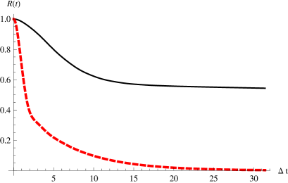
Figure 6: (Color online) Time evolution of the absolute value of Bloch vector for different values of the model parameters. The black solid line is the evolution for $\sigma_{a}=0.1\Delta$ and $\zeta_{a}=0.2\Delta$. Red dashed line $\sigma_{a}=0.5\Delta$ and $\zeta_{0}=0.75\Delta$. We have considered the effect of longitudinal and transverse noise simultaneously. We have set $\varphi_{\rm R}=0$ for simplicity, and the initial state is given by $\theta=\pi/3$.

In Fig.6 we present the temporal evolution of the absolute value of Bloch vector $\bf{R}$ while the qubit is evolving under the presence of $1/f$ noise. We consider $\sigma_{a}=0.1\Delta$ ($\zeta_{a}=0.2\Delta$) for the black solid line and $\sigma_{a}=0.5\Delta$ ($\zeta_{a}=0.75\Delta$) for the red dashed curve ($a=0,1$). We can see that as the value of $\sigma_{a}$ becomes bigger, the sooner purity is lost. This is so because $\sigma_{a}$ represents the coupling with the system ($a=0$ in the longitudinal coupling, and $a=1$ in the transverse case). Similar to the case of an Ohmic environment at high-T, the 1/f noise is very efficient in inducing decoherence on the system. The choice of parameters has been done to assure that there are no memory effects in the evolution, namely $\zeta>\sigma$ in our weak coupled model. In both cases, we see that purity is a monotonic decaying function.

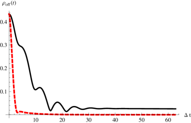
Figure 7: (Color online) Decay of the quantum coherences ($\rho_{r_{\text{off}}}(t)$), i.e the off diagonal terms of the reduced density matrix $\rho_{r_{01}}(t)$ as function of time. The lines correspond to the same values of Fig.6. We have considered the effect of longitudinal and transverse noise simultaneously. The initial state is given by $\theta=\pi/3$.

In order to have a rough estimation of the decoherence time, we consider only the longitudinal coupling and no anomalous diffusion terms (i.e. dephasing process). Then, assuming that $\zeta_{a}t\leq 1$, it is possible to show that $t_{D}\sim\sqrt{2}/\sigma_{a}$, independent of the switching rate. This fact can be clearly seen in Fig. 7, we have plotted the behaviour of the quantum coherences of the reduced density matrix as function of time. It is worthy to note these decoherence timescales are the temporal scale in which coherences abruptly decay from the pure-case value. This estimation sets a bound on the decoherence time. The asymptotic value is reached in a longer time. With the parameters used in Fig. 6, it is possible to check that decoherence time scales as $\Delta t_{D}\sim 3$ (red dashed line in Fig.7), and $\Delta t_{D}\sim 14$ (see black solid line in Fig. 7). On the contrary, when $\zeta_{a}t\gg 1$, decoherence time scales as $t_{D}\sim 1/\zeta_{a}$, almost independently of the value of $\sigma_{a}$.

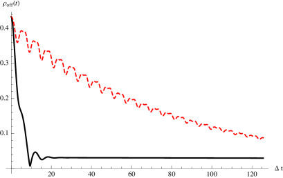
Figure 8: (Color online) Time evolution of the absolute value of Bloch vector in the Bloch sphere for different values of the model parameters. The red dashed line is the evolution for $\sigma_{1}=0.2\Delta$, $\zeta_{0}=0.5\Delta$, $\sigma_{0}=0$. The black solid line is for $\sigma_{0}=0.2\Delta$, $\zeta_{1}=0.5\Delta$, $\sigma_{1}=0$. We have set $\varphi_{\rm R}=0$ for simplicity. The initial state is given by $\theta=\pi/3$.

Finally, we consider the effect of noise in both directions as we have done for the Ohmic environments. It is important to note that in the case of $1/f$ noise, the coupling constant is included in parameter $\sigma_{a}$ of the model. Here, we will study the behaviour of the coherence $\rho_{r_{\text{off}}}(t)$ to infer how decoherence is induced in each case. In the following figures we present the behaviour of the quantum state for different coupling situations.

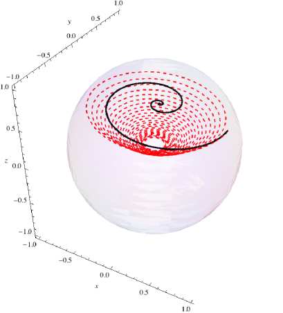
Figure 9: (Color online) Trajectories in the Bloch sphere for the values of the model parameters of Fig.8. The red dashed line is the evolution for $\sigma_{1}=0.2\Delta$, $\zeta_{0}=0.5\Delta$, $\sigma_{0}=0$. The black solid line is for $\sigma_{0}=0.2\Delta$, $\zeta_{1}=0.5\Delta$, $\sigma_{1}=0$. We have set $\varphi_{\rm R}=0$ for simplicity. The initial state is given by $\theta=\pi/3$

In Fig.8 we present the temporal evolution of the absolute value of Bloch vector $\bf{R}$ while the qubit is evolving under the presence of $1/f$ noise and in Fig.9 the trajectories in the Bloch sphere for the same model parameters. The red dashed line is the evolution for $\sigma_{1}=0.2\Delta$, $\zeta_{0}=0.5\Delta$, $\sigma_{0}=0$. The black solid line is for $\sigma_{0}=0.2\Delta$, $\zeta_{1}=0.5\Delta$, $\sigma_{1}=0$. This means that the black solid line represents a qubit coupled to the environment in a longitudinal direction only while the red dashed is the qubit coupled to the environment in the transverse direction only. It is easy to see in Fig.9 that the longitudinal coupling removes the state from the surface of the sphere rapidly by loosing purity faster (Fig.8). In the case of the transverse noise (red color), the effect of noise on the system may be neglected for very short times, by noting that the trajectory remains very similar to the unitary one in that timescale. The black solid line shows that having a coupling in the $\hat{z}$ direction removes the system for the Bloch sphere faster than having a coupling only in the $\hat{x}$ direction. This means that the purely dephasing process is the leading process when having both couplings together.

VI Final Remarks

The interaction of a solid-state qubit with environmental degrees of freedom strongly affects the qubit dynamics, and leads to decoherence. In quantum information processing with solid-state qubits, decoherence significantly limits the performance of such devices. These degrees of freedom appear as noise induced in the parameters entering the qubit Hamiltonian and also as noise in the control currents. These noise sources produce decoherence in the qubit, with noise, mainly, at microwave frequencies affecting the relative population between the ground and excited state, and noise or low-frequency fluctuations affecting the phase of the qubit. It is important to study the physical origins of decoherence by means of noise spectral densities and noise statistics. Therefore, it is necessary to fully understand the mechanisms that lead to decoherence.

We have derived a perturbative master equation for a superconducting qubit coupled to external sources of noise, including the combined effect of noise in the longitudinal and transversal directions. We have considered different types of noise by defining their correlation function in time. Decoherence can be understood as fluctuations in the Bloch vector ${\bf R}$ induced by noise. Since decoherence rate depends on the state of the qubit, we have represented decoherence by the change of $|{\bf R}|$ in time, starting from $|{\bf R}|=1$ for the initial pure state, and decreasing as long as the quantum state losses purity.

For an Ohmic environment, we have considered thermal effects. We have solved the master equation and presented the dynamics of the superconducting qubit in the presence of a high temperature environment and a zero temperature one. In both cases, we have computed the corresponding diffusion and dissipation coefficients, solved the master equation numerically and derived some analytical rough estimations of the decoherence time when possible. As expected, an environment at high temperature is an effective coherence destructor and a pure state vector is soon removed from the surface of the Bloch sphere. In addition, we have shown that decoherence is still induced in the qubit when the environment is at zero temperature. This process is less drastic and takes longer times compared to the high temperature limit. However, it is important to remark that the decoherence process still takes place, this time induced by the vacuum fluctuations of the environment. This fact has been shown for example in the loss of purity of the state vector and in the decay of the off-diagonal terms of the reduced density matrix, namely coherences. This result is in contrast to some recent publications pekola , where the effect of the environment at zero temperature is neglected. We have also focused on the effect of longitudinal and transversal noise. As expected, when the qubit is coupled to both directions, namely longitudinal and transverse, the influence of the environment is bigger as observed in the destruction of the coherences. However, it is important to note that having a transverse coupling only, does not imply a decoherence process as important as the one induced by the system when the coupling is longitudinal and the environment is at high temperature. This result is novel and should help in future qubits designs or experimental setups. Another important fact to take into account is that in the case of a zero-T environment, all noises are equally important at short times. This means that both noises affect the dynamics of the superconducting qubit in the same decoherence timescale as has been shown. The difference between couplings has not been studied before and this result is important when experimental setups are considered to be done in zero-T conditions.

We have also discussed the role of low-frequency of decoherence on quantum bits, namely a noise $1/f$, modelled herein by an ensemble of two-level fluctuators. We have presented this analysis in the framework of the master equation approach. From the definition of the noise correlation function of the environment, we have computed the diffusion coefficients and solved numerically the dynamics of the qubit. We have studied how this type of noise affects the coherences of the reduced density matrix and how the state vector is removed from the surface of the Bloch sphere. We have seen that this noise can be very destructive, depending on the value of the free parameter $\zeta$. We have provided some rough analytical estimations of the decoherence timescale that agree with the numerical solutions presented here. As for the effect of longitudinal and transversal noise, when the coupling is bidirectional the effect of noise is bigger on the coherences of the qubit.

The analysis of the decoherence timescales may provide additional information about the statistical properties of the noise. The comprehension of the decoherence and dissipative processes, origin and causes, should allow their further suppression in future qubits designs or experimental setups.

Appendix A

The functions $X_{a},Y_{a}$, and $Z_{a}$ appearing in Eq.(6) are derived by obtaining the temporal dependence of the Pauli operators $\sigma_{i}$ in the Heisenberg representing through the differential equations

$$\frac{d\sigma_{k}(t)}{dt}=i\left[H_{q},\sigma_{k}(t)\right],$$ (19)

with $k=x,y,z$ and $H_{\rm eff}$ as in Eq.(1). The solution can be expressed as a linear combination of the Pauli matrices (in the Schrödinger representation) as $\sigma_{z}^{a}=X_{a}(t)\sigma_{x}+Y_{a}(t)\sigma_{y}+Z_{a}(t)\sigma_{z}$. The explicit solution is given by

$$X_{1}(t) = \frac{\Omega_{x}^{2}+\left(\Delta^{2}+\Omega_{y}^{2}\right)\cos(2t\sqrt{\Omega_{\rm R}^{2}+\Delta^{2}})}{\Omega_{\rm R}^{2}+\Delta^{2}},$$

$$Y_{1}(t) = \frac{\Omega_{x}\Omega_{y}\left(1-\cos(2t\sqrt{\Omega_{\rm R}^{2}+\Delta^{2}})\right)+\Delta\sqrt{\Omega_{\rm R}^{2}+\Delta^{2}}\sin(2t\sqrt{\Omega_{\rm R}^{2}+\Delta^{2}})}{\Omega_{\rm R}^{2}+\Delta^{2}},$$

$$Z_{1}(t) = \frac{\Omega_{x}\Delta\left(1-\cos(2t\sqrt{\Omega_{\rm R}^{2}+\Delta^{2}})\right)-\Omega_{y}\sqrt{\Omega_{\rm R}^{2}+\Delta^{2}}\sin(2t\sqrt{\Omega_{\rm R}^{2}+\Delta^{2}})}{\Omega_{\rm R}^{2}+\Delta^{2}},$$

$$X_{2}(t) = \frac{\Omega_{x}\Omega_{y}\left(1-\cos(2t\sqrt{\Omega_{\rm R}^{2}+\Delta^{2}})\right)-\Delta\sqrt{\Omega_{\rm R}^{2}+\Delta^{2}}\sin(2t\sqrt{\Omega_{\rm R}^{2}+\Delta^{2}})}{\Omega_{\rm R}^{2}+\Delta^{2}},$$

$$Y_{2}(t) = \frac{\Omega_{y}^{2}+\left(\Delta^{2}+\Omega_{x}^{2}\right)\cos(2t\sqrt{\Omega_{\rm R}^{2}+\Delta^{2}})}{\Omega_{\rm R}^{2}+\Delta^{2}},$$

$$Z_{2}(t) = \frac{\Delta\Omega_{y}\left(1-\cos(2t\sqrt{\Omega_{\rm R}^{2}+\Delta^{2}})\right)+\Omega_{x}\sqrt{\Omega_{\rm R}^{2}+\Delta^{2}}\sin(2t\sqrt{\Omega_{\rm R}^{2}+\Delta^{2}})}{\Omega_{\rm R}^{2}+\Delta^{2}},$$

$$X_{0}(t) = \frac{\Delta\Omega_{x}\left(1-\cos(2t\sqrt{\Omega_{R}^{2}+\Delta^{2}})\right)+\Omega_{y}\sqrt{\Omega_{\rm R}^{2}+\Delta^{2}}\sin(2t\sqrt{\Omega_{R}^{2}+\Delta^{2}})}{\Omega_{R}^{2}+\Delta^{2}},$$

$$Y_{0}(t) = \frac{\Delta\Omega_{y}\left(1-\cos(2t\sqrt{\Omega_{R}^{2}+\Delta^{2}})\right)-\Omega_{x}\sqrt{\Omega_{\rm R}^{2}+\Delta^{2}}\sin(2t\sqrt{\Omega_{R}^{2}+\Delta^{2}})}{\Omega_{R}^{2}+\Delta^{2}},$$

$$Z_{0}(t) = \frac{\Delta^{2}+\Omega_{\rm R}^{2}\cos(2t\sqrt{\Omega^{2}+\Delta^{2}})}{\Omega_{\rm R}^{2}+\Delta^{2}}.$$

With these functions, we can evaluate all the coefficients in Eq.(6), and obtain the desired temporal evolution for each of the considered types of environment, defined through the spectral density.

References

- (1) M.A. Nielsen and I.L. Chuang, Quantum Computation and Quantum Information, Cambridge University Press, 2000.
- (2) J. P. Paz and W. H. Zurek, in Coherent Matter Waves, edited by R. Kaiser, C. Westbrook, and F. David, Proceedings of the Les Houches Summer School on Theoretical Physics, LXXII, 2000 (EDP Sciences/Springer, Berlin, 2001), pp. 533–614; W. H. Zurek, Rev. Mod. Phys. 75, 715 (2003).
- (3) U. Weiss, Quantum Dissipative Systems (World Scientific, Singapore, 1999).
- (4) F. C. Lombardo and P. I. Villar, Phys. Rev. A 72, 034103 (2005).
- (5) P. I. Villar and F. C. Lombardo, Phys. Rev. A 83, 052121 (2011).
- (6) F. C. Lombardo and P. I. Villar, Phys. Rev. A 87, 032338 (2013).
- (7) G. Ithier, E Collin, P. Joyez, P.J. Meeson, D. Vion, D. Esteve, F. Chiarello, A. Shnirman, Y. Makhlin, J. Schriefl, and G. Schon, Phys. Rev. B 72, 134519 (2005).
- (8) E. Paladino, Y. M. Galperin, G. Falci and B. L. Altshuler, Rev. Mod. Phys. 86, 361 (2014).
- (9) A.I. Nesterov and G.P. Berman, Phys. Rev. A 85, 052125 (2012).
- (10) Dong Zhou and Robert Joynt, Supercond. Sci. Technol., 25, 045003 (2012).
- (11) P. Solinas, M. Mottonen, J. Salmilehto, and J. P. Pekola, Phys. Rev. B 82, 134517 (2010); J. P. Pekola, V. Brosco, M. Mottonen, P. Solinas, and A. Shnirman, Phys. Rev. Lett. 105, 030401(2010).
- (12) F. C. Lombardo and P. I. Villar, Physics Letters A 336, 16, (2005).
- (13) F.C. Lombardo and P.I.Villar, Physics Letters A 371, 190, (2007).
- (14) Nuno D. Antunes, Fernando C. Lombardo, Diana Monteoliva, and Paula I. Villar, Phys. Rev. E 73, 066105 (2006).
- (15) Luciana Dávila Romero and Juan Pablo Paz, Phys. Rev. A 55, 4070 (1997).
- (16) John M. Martinis, S. Nam, J. Aumentado, and K.M. Lang, Phys. Rev. B 67, 094510 (2003).
- (17) Yuriy Makhlin, Gerd Schoen, and Alexander Shnirman, Rev. Mod. Phys. 73, 357 (2001).
- (18) S. Berger, M. Pechal, A.A. Adbumalikov, Jr, C. Eichler, L. Steffen, A. Fedorov, A. Wallraff, and S. Filipp, Phys. Rev. A 87, 060303 (R) (2013).
- (19) B. D. Josephson, Rev. Mod. Phys. 46, 251 (1974).
- (20) P. J. Leek, J. M. Fink, A. Blais, R. Bianchetti, M. Göppl, J. M. Gambetta, D. I. Schuster, L. Frunzio, R. J. Schoelkopf, A. Wallraff1, Science 318, 1889 (2007).
- (21) Fernando C. Lombardo and Paula I. Villar, Phys. Rev. A 89, 012110 (2014).
- (22) Heinz-Peter Breuer and Francesco Petruccione, The Theory of Open Quantum Systems, OUP Oxford, 2007.
- (23) A.J. Leggett, S. Chakravarty, A. T. Dorsey, M. P. A. Fisher, A. Garg,. W. Zwerger, Rev. Mod. Phys. 59, 1 (1987).
- (24) F.C. Lombardo and P.I. Villar, Phys. Rev. A 74, 042311 (2006).
- (25) G. Benenti, G. Casati, G. Strini, Principles of Quantum Computation and Information, World Scientific Publishing Co. Pte. Ltd, 2004. Science 296, 886 (2002).
- (26) Martin V. Gustafsson, Arsalan Pourkabirian, Goran Johansson, John Clarke, and Per Delsing, Phys. Rev. B 88, 245410 (2013).
- (27) Henry J. Wold, Hakon Brox, Yuri M. Galperin, and Joakim Bergli, Phys. Rev. B 86, 205404 (2012).