Metric recovery from directed unweighted graphs

Abstract

We analyze directed, unweighted graphs obtained from $x_{i}\in\mathbb{R}^{d}$ by connecting vertex $i$ to $j$ iff $|x_{i}-x_{j}|<\varepsilon(x_{i})$. Examples of such graphs include $k$-nearest neighbor graphs, where $\varepsilon(x_{i})$ varies from point to point, and, arguably, many real world graphs such as co-purchasing graphs. We ask whether we can recover the underlying Euclidean metric $\varepsilon(x_{i})$ and the associated density $p(x_{i})$ given only the directed graph and $d$.

We show that consistent recovery is possible up to isometric scaling when the vertex degree is at least $\omega(n^{2/(2+d)}\log(n)^{d/(d+2)})$. Our estimator is based on a careful characterization of a random walk over the directed graph and the associated continuum limit. As an algorithm, it resembles the PageRank centrality metric. We demonstrate empirically that the estimator performs well on simulated examples as well as on real-world co-purchasing graphs even with a small number of points and degree scaling as low as $\log(n)$.

1 Introduction

Data for unsupervised learning is increasingly available in the form of graphs or networks. For example, we may analyze gene networks, social networks, or general co-occurrence graphs (e.g., built from purchasing patterns). While classical unsupervised tasks such as density estimation or clustering are naturally formulated for data in vector spaces, these tasks have analogous problems over graphs such as centrality and community detection. We provide a step towards unifying unsupervised learning by recovering the underlying density and metric directly from graphs.

We consider “unweighted directed geometric graphs” that are assumed to have been built from underlying (unobserved) points $x_{i}$, $i=1,\ldots,n$. In particular, we assume that graphs are formed by drawing an arc from each vertex $i$ to its neighbors within distance $\varepsilon_{n}(x_{i})$. Note that the graphs are typically not symmetric since the distance (the $\varepsilon_{n}$-ball) may vary from point to point. By allowing $\varepsilon_{n}(x_{i})$ to be stochastic, e.g., depend on the set of points, the construction subsumes also typical $k$-nearest neighbor graphs. Arguably, graphs from top $k$ friends/products, or co-association graphs may also be approximated in this manner.

The key property of our family of geometric graphs is that their structure is completely characterized by two functions over the latent space: the local density $p(x)$ and the local scale $\varepsilon(x)$. Indeed, global properties such as the distances between points can be recovered by integrating these quantities. We show that asymptotic behavior of random walks on the directed graphs relate to the density and metric. In particular, we show that random walks on such graphs with minimal degree at least $\omega(n^{2/(2+d)}\log(n)^{\frac{d}{d+2}})$ can be completely characterized in terms of $p$ and $\varepsilon$ using drift-diffusion processes. This enables us to recover both the density and distance given only the observed graph and the (hypothesized) underlying dimension $d$.

The fact that we may recover the density (up to isometry) is surprising. For example, in $k$-nearest neighbor graphs, each vertex has degree exactly $k$. There is no immediate local information about the density, i.e., whether the corresponding point lies in a high-density region with small ball radii, or in a low-density region with large ball radii. The key insight of this paper is that random walks over such graphs naturally drift toward higher density regions, allowing for density recovery.

While the paper is primarily focused on the theoretical aspects of recovering the metric and density, we believe our results offer useful strategies for analyzing real-world networks. For example, we analyzed the Amazon co-purchasing graph where an edge is drawn from an item $i$ to $j$ if $j$ is among the top $k$ co-purchased items with $i$. These Amazon products may be co-purchased if they are similar enough to be complementary, but not so similar that they are redundant. We extend our model to deal with connectivity rules shaped like an annulus, and demonstrate that our estimator can simultaneously recover product similarities, product categories, and central products by metric embedding.

1.1 Relation to prior work

The density estimation problem addressed by this paper was proposed and partially solved by von Luxburg-Alamgir in [14] using integration of local density gradients over shortest paths. This estimator has since been used for drawing graphs with ordinal constraints in [14] and graph down-sampling in [1]. However, the recovery algorithm is restricted to $1$-dimensional $k$-nearest neighbor graphs under the constraint $k=\omega(n^{2/3}\log(n)^{\frac{1}{3}})$. Our paper provides an estimator that works in all dimensions, applies to a more general class of graphs, and strongly outperforms that of von Luxburg-Alamgir in practice.

On a technical level, our work has similarities to the analysis of convergence of graph Laplacians and random walks on manifolds in [16, 6]. For example, in [13], Ting-Huang-Jordan used infinitesimal generators to capture the convergence of a discrete Laplacian to its continuous equivalent on $k$-nearest neighbor graphs. However, their analysis was restricted to the Laplacian and did not consider the latent recovery problem. In addition, our approach proves convergence of the entire random walk trajectory and allows us to analyze the stationary distribution function directly.

2 Main results and proof outline

2.1 Problem setup

Let $\mathcal{X}=\{x_{1},x_{2},\ldots\}$ be an infinite sequence of latent coordinate points drawn independently from a distribution with probability density $p(x)$ in $\mathbb{R}^{d}$. Let $\varepsilon_{n}(x_{i})$ be a radius function which may depend on the draw of $\mathcal{X}$. In this paper, we fix a single draw of $\mathcal{X}$ and analyze the quenched setting. Let $G_{n}=(\mathcal{X}_{n},E_{n})$ be the unweighted directed neighborhood graph with vertex set $\mathcal{X}_{n}=\{x_{1},\ldots,x_{n}\}$ and with a directed edge from $i$ to $j$ if and only if $|x_{i}-x_{j}|<\varepsilon_{n}(x_{i})$.

Fix now a large $n$. We consider the random directed graph model given by observing the single graph $G_{n}$. The model is completely specified by the latent function $p(x)$ and the possibly stochastic $\varepsilon_{n}(x)$. Under the conditions ($\star$) to be specified below, we solve the following problem:

• Given only $G_{n}$ and $d$, form a consistent estimate of $p(x_{i})$ and $|x_{i}-x_{j}|$ up to proportionality constants.

The conditions we impose on $p(x)$, $\varepsilon_{n}(x)$, and the stationary density function $\pi_{X_{n}}(x)$ of the simple random walk $X_{n}(t)$ on $G_{n}$ are the following, which we refer to as ($\star$). We assume ($\star$) holds throughout the paper.

• The density $p(x)$ is differentiable with bounded $\nabla\log(p(x))$ on a path-connected compact domain $D\subset\mathbb{R}^{d}$ with smooth boundary $\partial D$.

• There is a deterministic continuous function $\overline{\varepsilon}(x)>0$ on $\overline{D}$ and scaling constants $g_{n}$ satisfying

  $$g_{n}\to 0\text{ and }g_{n}n^{\frac{1}{d+2}}\log(n)^{-\frac{1}{d+2}}\to\infty$$

  so that, a.s. in the draw of $\mathcal{X}$, $g_{n}^{-1}\varepsilon_{n}(x)$ converges uniformly to $\overline{\varepsilon}(x)$.

• The rescaled density functions $n\pi_{X_{n}}(x)$ are a.s. uniformly equicontinuous.

Remark.

We conjecture that the last condition in ($\star$) holds for any $p$ and $\overline{\varepsilon}$ satisfying the other conditions in ($\star$) (see Conjecture SLABEL:Sconj:holder).

Let $\mathsf{NB}_{n}(x)$ denote the set of out-neighbors of $x$ so that $y$ is in $\mathsf{NB}_{n}(x)$ if there is a directed edge from $x$ to $y$. The second condition in ($\star$) implies for all $x\in\mathcal{X}_{n}$ that

$$|\mathsf{NB}_{n}(x)|=\omega(n^{\frac{2}{d+2}}\log(n)^{\frac{d}{d+2}}).$$ (1)

2.2 Statement of results

Our approach is based on the simple random walk $X_{n}(t)$ on the graph $G_{n}$. Let $\pi_{X_{n}}(x)$ denote the stationary density of $X_{n}(t)$. We first show that when appropriately renormalized, $\pi_{X_{n}}(x)$ converges to an explicit function of $p(x)$ and $\overline{\varepsilon}(x)$.

Theorem 2.1.

Given ($\star$), a.s. in $\mathcal{X}$, we have

$$n\pi_{X_{n}}(x)\rightarrow c\frac{p(x)}{\overline{\varepsilon}(x)^{2}},$$ (2)

for the normalization constant $c^{-1}=\int p(x)^{2}\overline{\varepsilon}(x)^{-2}dx$.

Combining this result with an estimate on the out-degree of points in $G_{n}$ gives our general result on recovery of density and scale. Let $V_{d}$ be the volume of the unit $d$-ball.

Corollary 2.2.

Assuming ($\star$), we have a.s. in $\mathcal{X}$ that

$$\left(\frac{n^{\frac{d-2}{d}}}{cV_{d}^{2/d}g_{n}^{2}}\right)^{\frac{d}{d+2}}|\mathsf{NB}_{n}(x)|^{\frac{2}{d+2}}\pi_{X_{n}}(x)^{\frac{d}{d+2}} \rightarrow p(x)\text{ and}$$

$$\left(\frac{1}{c^{d/2}V_{d}n^{2}g_{n}^{d}}\right)^{\frac{1}{d+2}}|\mathsf{NB}_{n}(x)|^{\frac{1}{d+2}}\pi_{X_{n}}(x)^{-\frac{1}{d+2}} \to\overline{\varepsilon}(x).$$

Proof.

Immediate from the out-degree estimate $p(x)\varepsilon_{n}(x)^{d}V_{d}=|\mathsf{NB}_{n}(x)|/n$ and Theorem 2.1. ∎

Remark.

If $\varepsilon_{n}(x)$ is constant, every edge is bidirectional, so $\pi_{X_{n}}(x)$ is proportional to the degree of $x$, and we recover the standard $\varepsilon$-ball density estimator.

Our estimator for density $p(x)$ closely resembles the PageRank algorithm without damping [10]. In particular, for the $k$-nearest neighbor graph, it gives the same rank ordering as PageRank, and it reduces to PageRank as $d\to\infty$.

When specializing to the $k$-nearest neighbor density estimation problem posed by von Luxburg-Alamgir in [14], we obtain the following.

Corollary 2.3.

If $\varepsilon_{n}(x)$ is selected via the $k$-nearest neighbors procedure with $k=\omega(n^{\frac{2}{d+2}}\log(n)^{\frac{d}{d+2}})$ and satisfies the first and last conditions in ($\star$), we have a.s in $\mathcal{X}$ that

$$\left(\frac{n}{cV_{d}^{2/d}}\right)^{\frac{d}{d+2}}\pi_{X_{n}}(x)^{\frac{d}{d+2}} \rightarrow p(x)\text{ and}$$

$$\left(\frac{1}{c^{d/2}V_{d}n}\right)^{\frac{1}{d+2}}\pi_{X_{n}}(x)^{-\frac{1}{d+2}} \rightarrow\overline{\varepsilon}(x).$$

Proof.

By [4], the empirical $\varepsilon_{n}(x)$ induced by the $k$-nearest neighbors procedure satisfies the second condition of ($\star$) with

$$\overline{\varepsilon}(x)=\frac{1}{V_{d}^{1/d}p(x)^{1/d}}\text{ and }g_{n}=(k/n)^{1/d}.\qed$$

2.3 Outline of approach

Our proof proceeds via the following steps.

1. As $n\to\infty$, the simple random walks $X_{n}(t)$ on $G_{n}$ converge weakly to an Itô process $Y(t)$, yielding weak convergence between stationary measures. (Theorem 3.4)

2. The stationary density $\pi_{Y}(x)$ is explicitly determined via Fokker-Planck equation. (Lemma 4.1)

3. Uniform equicontinuity of $n\pi_{X_{n}}(x)$ yields convergence in density after rescaling. (Theorem 2.1)

An intuitive explanation for our results is as follows. For large $n$, the simple random walk on $G_{n}$, when considered with its original metric embedding, closely approximates the behavior of a drift-diffusion process. Both the process and the approximating walk move preferentially toward regions where $p(x)$ is large and diffuse more slowly out of regions where $\overline{\varepsilon}(x)$ is small. Occupation times therefore give us information about $p(x)$ and $\overline{\varepsilon}(x)$ which allow us to recover them.

Formally, the convergence of $X_{n}(t)$ to $Y(t)$ follows by verifying the conditions of the Stroock-Varadhan criterion (Theorem 3.1) for convergence of discrete time Markov processes to Itô processes [12]. This criterion states that if the variance $a_{n}$, expected value $b_{n}$, a higher order moments $\Delta_{n,\alpha}$ of a jump are continuous and well-controlled in the limit, then the process converges to an Itô process under mild technical conditions. By using the Fokker-Planck equation, we can express the stationary density of this Itô process solely in terms of $p(x)$ and the out-degree $|\mathsf{NB}_{n}(x)|$. This allows us to estimate the density using only the unweighted graph.

Let $\overline{D}$ and $\partial D$ be the closure and boundary of the support $D$ of $p(x)$. Let $B(x,\varepsilon)$ be the ball of radius $\varepsilon$ centered at $x$. Let $h_{n}=g_{n}^{2}$ be the time rescaling necessary for $X_{n}(t)$ to have timescale equal to that of $Y(t)$.

3 Convergence of the simple random walk to an Itô process

We will verify the regularity conditions of the Stroock-Varadhan criterion (see [12, Section 6]).

Theorem 3.1 (Stroock-Varadhan).

Let $X_{n}(t)$ be discrete-time Markov processes defined over a domain $D$ with boundary $\partial D$. Define the discrete time drift and diffusion coefficients by

$$a_{n}^{ij}(s,x) =\frac{1}{h_{n}}\sum_{y\in\mathsf{NB}_{n}(x)}\frac{1}{|\mathsf{NB}_{n}(x)|}(y_{i}-x_{i})(y_{j}-x_{j})$$

$$b_{n}^{i}(s,x) =\frac{1}{h_{n}}\sum_{y\in\mathsf{NB}_{n}(x)}\frac{1}{|\mathsf{NB}_{n}(x)|}(y_{i}-x_{i})$$

$$\Delta_{n,\alpha}(s,x) =\frac{1}{h_{n}}\sum_{y\in\mathsf{NB}_{n}(x)}\frac{1}{|\mathsf{NB}_{n}(x)|}|y-x|^{2+\alpha}.$$

If we have $a_{n}^{ij}(s,x)\xrightarrow{a.s}a^{ij}(s,x)$, $b_{n}^{i}(s,x)\xrightarrow{a.s}b^{i}(s,x)$, $\Delta_{n,1}(s,x)\xrightarrow{a.s}0$, and regularity conditions to ensure reflection at $\partial D$ (Theorem SLABEL:Sthm:tightness and Theorem SLABEL:Sthm:stroock), the time-rescaled stochastic processes $X_{n}(\lfloor t/h_{n}\rfloor)$ converge weakly in Skorokhod space $\mathsf{D}([0,\infty),\overline{D})$ to an Itô process with reflecting boundary condition

$$dY(t)=\sigma(t,Y(t))dW_{t}+b(t,Y(t))dt,$$

with $W_{t}$ a standard $d$-dimensional Brownian motion and $\sigma(t,Y(t))\sigma(t,Y(t))^{T}=a(t,Y(t))$.

Remark.

The original result of Stroock-Varadhan was stated for $\mathsf{D}([0,T],\overline{D})$ for all finite $T$; our version for $\mathsf{D}([0,\infty),\overline{D})$ is equivalent by [15, Theorem 2.8].

The technical conditions of Theorem 3.1 enforcing reflecting boundary conditions are checked in Theorem SLABEL:Sthm:C to Theorem SLABEL:Sthm:B. We focus on convergence of the drift and diffusion coefficients.

Lemma 3.2 (Strong LLN for local moments).

For a function $f(x)$ such that $\sup_{x\in B(0,\varepsilon)}|f(x)|<\varepsilon$, given ($\star$) we have uniformly on $x\in\mathcal{X}_{n}$ that

$$\frac{1}{h_{n}}\sum_{y\in\mathsf{NB}_{n}(x)}\frac{1}{|\mathsf{NB}_{n}(x)|}f(y-x)$$

$$\qquad\xrightarrow{a.s.}\frac{1}{h_{n}}\int_{y\in B(x,\varepsilon_{n}(x))}f(y-x)\frac{p(y)}{p_{\varepsilon_{n}(x)}(x)}dy.$$

Proof.

Denote the claimed value of the limit by $\mu(x)$. For convergence in expectation, we condition on $|\mathsf{NB}_{n}(x)|$ and apply iterated expectation to get

$$E\left[\frac{1}{h_{n}}\sum_{y\in\mathsf{NB}_{n}(x)}\frac{1}{|\mathsf{NB}_{n}(x)|}f(y-x)\right]$$

$$\qquad=E\left[\frac{1}{h_{n}}E\left[f(y-x)\big{|}|\mathsf{NB}_{n}(x)|\right]\right]=\mu(x).$$

For $y\in B(x,\varepsilon_{n}(x))$, we have $|f(y-x)|\leq\varepsilon_{n}(x)$, so Hoeffding’s inequality yields

$$P\bigg{(}\bigg{|}\frac{1}{h_{n}} \sum_{y\in\mathsf{NB}_{n}(x)}\frac{1}{|\mathsf{NB}_{n}(x)|}f(y-x)-\mu(x)\bigg{|}\geq t\bigg{)}$$

$$\leq 2\exp\left(-\frac{2h_{n}^{2}|\mathsf{NB}_{n}(x)|^{2}t^{2}}{|\mathsf{NB}_{n}(x)|\varepsilon_{n}(x)^{2}}\right)$$

$$=\Theta\left(\exp\left(-2g_{n}^{2}\overline{\varepsilon}(x)^{-2}|\mathsf{NB}_{n}(x)|t^{2}\right)\right)$$ (3)

$$=o\left(n^{-\frac{2p(x)^{2/d}t^{2}}{\overline{\varepsilon}(x)^{4}}\omega(1)}\right)$$

$$=o(n^{-2t^{2}\omega(1)})$$

for $|\mathsf{NB}_{n}(x)|=\omega\left(n^{2/(d+2)}\log(n)^{d/(d+2)}\right)$ by (1). Borel-Cantelli then yields a.s. convergence. ∎

Remark.

This limit holds even for stochastic $\varepsilon_{n}(x)$ as long as $g_{n}^{-1}\varepsilon_{n}(x)$ a.s. converges uniformly to a deterministic continuous $\overline{\varepsilon}(x)$. All statements up to (3) hold regardless of stochasticity of $\varepsilon_{n}(x)$ and the overall bound only requires convergence of $\varepsilon_{n}(x)$. An example of such a graph is the $k$-nearest neighbors graph.

We now compute the drift and diffusion coefficients in terms of $p(x)$ and $\overline{\varepsilon}(x)$.

Theorem 3.3 (Drift diffusion coefficients).

Almost surely on the draw of $\mathcal{X}$, as $n\to\infty$, we have

$$\lim_{n\to\infty}a^{ij}_{n}(s,x) =\delta_{ij}\frac{1}{3}\overline{\varepsilon}(x)^{2}$$

$$\lim_{n\to\infty}b^{i}_{n}(s,x) =\frac{\partial_{i}p(x)}{3p(x)}\overline{\varepsilon}(x)^{2}$$

$$\lim_{n\to\infty}\Delta_{n,1}(s,x) =0,$$

where $\delta_{ij}$ is the Kronecker delta function.

Proof.

By Lemma 3.2, $a_{n}$, $b_{n}$, and $\Delta_{n,1}$ converge a.s. to their expectations, so it suffices to verify that the integrals in Lemma 3.2 have the claimed limits. Because $p$ is differentiable on $D$, for any $x\in D$ we have the Taylor expansion

$$p(x+y)=p(x)+y\cdot\nabla p(x)+o(|y|^{2})$$

of $p$ at $x$, where the convergence is uniform on compact sets. For $n$ large so that $B(x,\varepsilon_{n}(x))$ lies completely inside $D$, substituting this expansion into the definitions of $a_{n}$, $b_{n}$, and $\Delta_{n,1}$ and integrating over spheres yields the result. Full details are in Theorem SLABEL:Sthm:coefs. ∎

Theorem 3.4.

Under ($\star$), as $n\rightarrow\infty$ a.s. in the draw of $\mathcal{X}$ the process $X_{n}(\lfloor t/h_{n}\rfloor)$ converges in $\mathsf{D}([0,\infty),\overline{D})$ to the isotropic $\overline{D}$-valued Itô process $Y(t)$ with reflecting boundary condition defined by

$$dY(t)=\frac{\nabla p(Y(t))}{3p(Y(t))}\overline{\varepsilon}(Y(t))^{2}dt+\frac{\overline{\varepsilon}(Y(t))}{\sqrt{3}}dW(t).$$ (4)

Proof.

Lemma 3.2 and Theorem 3.3 show that $X_{n}(\lfloor t/h_{n}\rfloor)$ fulfills the conditions of Theorem 3.1. The result follows from the Stroock-Varadhan criterion using the drift and diffusion terms from Theorem 3.3. ∎

4 Convergence and computation of the stationary distribution

4.1 Graphs satisfying condition ($\star$)

The Itô process $Y(t)$ is an isotropic drift-diffusion process, so the Fokker-Planck equation [11] implies its density $f(t,x)$ at time $t$ satisfies

$$\partial_{t}f(t,x)=\sum_{i}\bigg{(}-\partial_{x_{i}}[b^{i}(t,x)f(t,x)]+\frac{1}{2}\partial_{x_{i}^{2}}[a^{ii}(t,x)f(t,x)]\bigg{)},$$ (5)

where $b^{i}(t,x)$ and $a^{ii}(t,x)$ are given by

$$b(t,x)=\frac{\nabla p(x)}{3p(x)}\bar{\varepsilon}(x)^{2}\text{ and }a^{ii}(t,x)=\frac{1}{3}\bar{\varepsilon}(x)^{2}.$$

Lemma 4.1.

The process $Y(t)$ defined by (4) has absolutely continuous stationary measure with density

$$\pi_{Y}(x)=cp(x)^{2}\overline{\varepsilon}(x)^{-2},$$

where $c$ was defined in (2).

Proof.

By (5), to check that $\pi_{Y}(x)=cp(x)^{2}\overline{\varepsilon}(x)^{-2}$, it suffices to show

$$\sum_{i}\bigg{(}\partial_{x_{i}}p(x)\left(p(x)^{-1}\overline{\varepsilon}(x)^{2}c\frac{p(x)^{2}}{\overline{\varepsilon}(x)^{2}}\right)-\frac{1}{2}\partial_{x_{i}}\left(\overline{\varepsilon}(x)^{2}c\frac{p(x)^{2}}{\overline{\varepsilon}(x)^{2}}\right)\bigg{)}=0.\qed$$

We now prove Theorem 2.1 by showing that a rescaling of $\pi_{X_{n}}(x)$ converges to $\pi_{Y}(x)$.

Proof of Theorem 2.1.

The a.s. convergence of processes of Theorem 3.4 implies by Ethier-Kurtz [5, Theorem 4.9.12] that the empirical stationary measures

$$d\mu_{n}=\sum_{i=1}^{n}\pi_{X_{n}}(x_{i})\delta_{x_{i}}$$

converge weakly to the stationary measure $d\mu=\pi_{Y}(x)dx$ for $Y(t)$. For any $x\in\mathcal{X}$ and $\delta>0$, weak convergence against $1_{B(x,\delta)}$ yields

$$\sum_{y\in\mathcal{X}_{n},|y-x|<\delta}\pi_{X_{n}}(y)\to\int_{|y-x|<\delta}\pi_{Y}(y)dy.$$

By uniform equicontinuity of $n\pi_{X_{n}}(x)$, for any $\varepsilon>0$ there is small enough $\delta>0$ so that for all $n$ we have

$$\left|\sum_{y\in\mathcal{X}_{n},|y-x|<\delta}\!\!\!\!\pi_{X_{n}}(y)-|\mathcal{X}_{n}\cap B(x,\delta)|\pi_{X_{n}}(x)\right|\leq n^{-1}|\mathcal{X}_{n}\cap B(x,\delta)|\varepsilon,$$

which implies that

$$\lim_{n\to\infty} \pi_{X_{n}}(x)p(x)n$$

$$=\lim_{\delta\to 0}\lim_{n\to\infty}V_{d}^{-1}\delta^{-d}n\pi_{X_{n}}(x)\int_{|y-x|<\delta}p(y)dy$$

$$=\lim_{\delta\to 0}\lim_{n\to\infty}V_{d}^{-1}\delta^{-d}|\mathcal{X}_{n}\cap B(x,\delta)|\pi_{X_{n}}(x)$$

$$=\lim_{\delta\to 0}V_{d}^{-1}\delta^{-d}\int_{|y-x|<\delta}\pi_{Y}(y)dy=\pi_{Y}(x).$$

Combining with Lemma 4.1 yields the desired

$$\lim_{n\to\infty}n\pi_{X_{n}}(x)=\frac{\pi_{Y}(x)}{p(x)}=c\frac{p(x)}{\overline{\varepsilon}(x)^{2}}.\qed$$

4.2 Extension to isotropic graphs

To obtain our stationary distribution in Theorem 2.1 we require only convergence to some Itô process via the Stroock-Varadhan criterion. We can achieve this under substantially more general conditions. We define a class of neighborhood graphs on $\mathcal{X}_{n}$ termed isotropic over which we have consistent metric recovery without knowledge of the graph construction method.

Definition 1 (Isotropic).

A graph edge connection procedure on $\mathcal{X}_{n}$ is isotropic if it satisfies:

Distance kernel:

The probability of placing a directed edge from $i$ to $j$ is defined by a kernel function $h(r_{ij})$ mapping locally scaled distances

$$r_{ij}=|x_{i}-x_{j}|\varepsilon_{n}(x_{i})^{-1}$$

with $\varepsilon_{n}(x)$ obeying ($\star$) to probabilities

Nonzero mass:

The kernel function $h(r)$ has nonzero integral $\int_{0}^{1}h(r)r^{d-1}dr>0$.

Bounded tails:

For all $r>1$, $h(r)=0$.

Continuity:

The scaling $n\pi_{X_{n}}(x)$ of the stationary distribution is uniformly equicontinuous.

This class of graph preserves the property that the random graph is entirely determined by the underlying density $p(x)$ and local scale $\overline{\varepsilon}(x)$; this allows us to have the same tractable form for the stationary distribution.

Both constant $\varepsilon$ and $k$-nearest neighbor graphs are isotropic upon assumption of uniform equicontinuity. Another interesting class of graphs allowed by this generalization is truncated Gaussian kernels, where connectivity probability decreases exponentially. Note that $h(r)$ might not be monotonic or continuous in $r$; one surprising example is $h(r)=1_{[0.5,1]}(r)$, which deterministically connects points in an annulus.

Corollary 4.2 (Generalization).

If a neighborhood graph is isotropic, then the limiting stationary distribution follows Theorem 2.1, and the density and distances can be estimated by Corollary 2.2.

Proof.

We check the Stroock-Varadhan condition stated in Theorem 3.1. For this, we use a version of Lemma 3.2 for isotropic graphs, which requires that the ball radius vanishes and that the neighborhood size scales as $\omega(n^{\frac{2}{d+2}}\log(n)^{\frac{d}{d+2}})$.

Vanishing neighborhood radius follows because bounded tails and the fact that the kernel is evaluated on $|x_{i}-x_{j}|\varepsilon_{n}(x_{i})^{-1}$ ensure the isotropic graph is a subgraph of the $\varepsilon_{n}(x)$-ball graph. Kolmogorov’s strong law implies that the stochastic out-degree concentrates around its expectation. It has the correct scaling because the argument of $h(r)$ is scaled by $\varepsilon_{n}(x)$. See Theorem SLABEL:Sthm:general-degree for details. Thus the analogue of Lemma 3.2 holds.

We then check that the limiting local moments for isotropic graphs are proportional to those of $\varepsilon_{n}(x)$-ball graphs in Lemma SLABEL:Slem:polyint. All but one of the conditions for the Stroock-Varadhan criterion follow from this; the last Theorem SLABEL:Sthm:f4 follows from the bounded ball structure of the connectivity kernel.

To check that we obtain the same limiting process and stationary measure, note the ratios of integrals in Theorem 3.3 are unchanged in the isotropic setting. See Lemma SLABEL:Slem:polyint for details. Recovering the stationary distribution, density, and local scale is then done in the same manner as in the $\varepsilon$-ball setting. ∎

5 Distance recovery via paths

Our results in Theorem 2.1 give a consistent estimator for the density $p(x)$ and the local scale $\overline{\varepsilon}(x)$. These two quantities specify up to isometry the latent metric embedding of $\mathcal{X}$.

In order to reconstruct distances between non-neighbor points we weight the edges of $G_{n}$ by weights $w_{ij}=\varepsilon_{n}(x_{i})$ and find the shortest paths over this graph, which we call $\overline{G}_{n}$. The results of Alamgir-von Luxburg [2, Section 4.1] show that in the $k$-nearest neighbor graph case, setting $w_{ij}=\widehat{\varepsilon}_{n}(x_{i})$ for the estimator $\widehat{\varepsilon}_{n}$ of $\varepsilon_{n}$ results in consistent recovery of pairwise distances.

In Theorem SLABEL:Sthm:dist, we give a straightforward extension of this approach to show that given any uniformly convergent estimator of $\varepsilon_{n}(x)$, the shortest path on the weighted graph $\overline{G}_{n}$ converges to the geodesic distance. Applying standard metric multidimensional scaling then allows us to embed these distances and recover the latent space up to isometry.

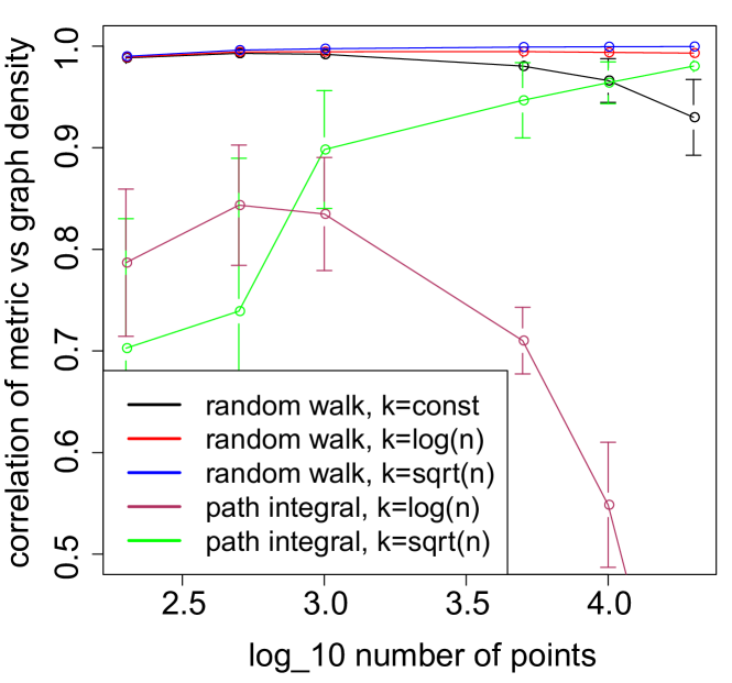
Figure 1: Accuracy vs sample and neighborhood size. Path integral (green, maroon) is from Alamgir-von Luxburg [14]. Our estimator (red, blue, black) is nearly perfect at all sample sizes and neighborhood sizes.

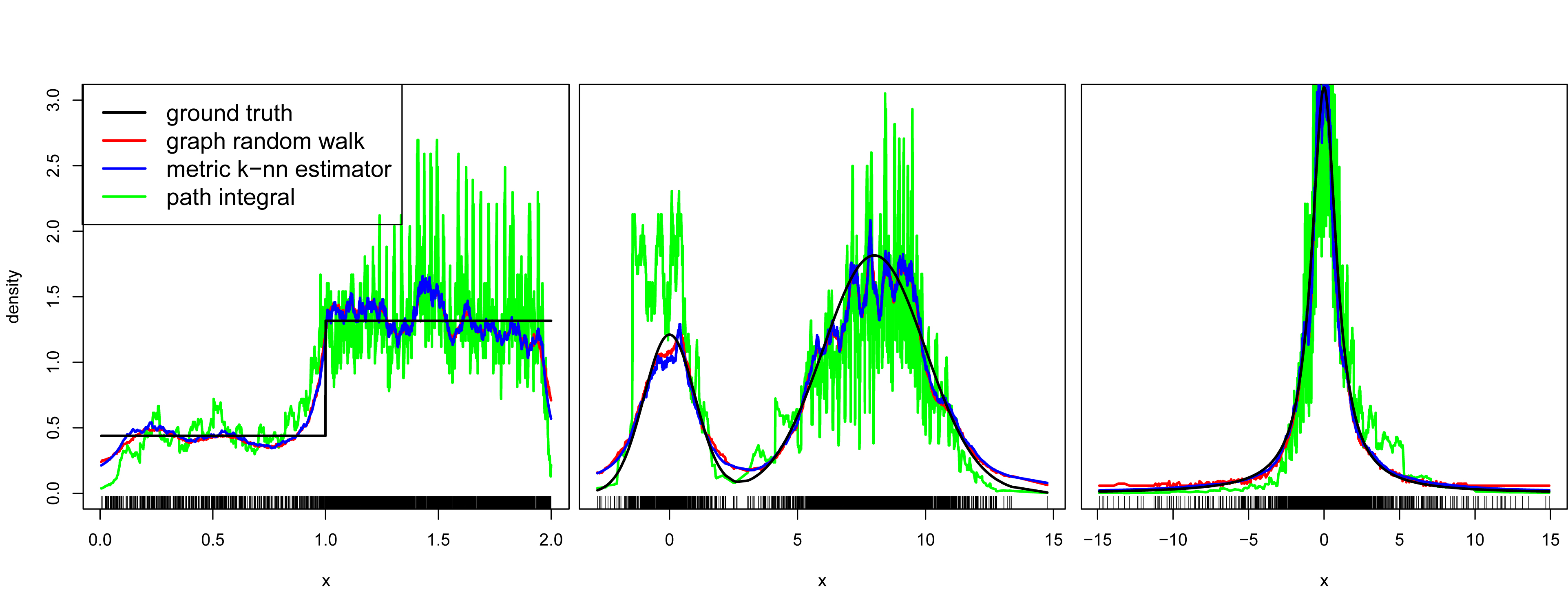
Figure 2: Examples of four density estimates: our method (red) using no metric information is indistinguishable from metric $k$-nearest neighbor (blue) and close to ground truth (black). Path integral estimator of Alamgir-von Luxburg [14] (green) shows higher error in all cases.

6 Empirical results

We demonstrate extremely good finite sample performance of our estimator in simulated density reconstruction problems and two real-world datasets. Some details such as exact graph degrees and distribution parameters are in the supplementary code which reproduces all figures in this paper. Standard graph statistics such as centrality and Jaccard index are calculated via the igraph package [3].

$k$-nearest neighbor graphs

We compared our random-walk based estimator and the path-integral based estimator of von Luxburg-Alamgir [14] to the metric $k$-nearest neighbor density estimator. The number of samples $n$ was varied from $100$ to $20000$ along with the sparsity level $k$ (Figure 2).

While our theoretical results suggest that both our algorithm and the path-integral estimator of von Luxburg-Alamgir [14] might fail to converge at $\sqrt{n}$ and $\log(n)$ sparsity levels, in practice our estimator performs nearly perfectly at both low sparsity levels.

For constant degree $k=50$ we achieve near-perfect performance for all choices of $n$, while the path-integral estimator fails to converge in the $k=\log(n)$ regime.

Some specific examples of our density estimator with $n=2000,k=100$ are shown in Figure 2. The examples are mixture of uniforms (left), mixture of Gaussians (center), and $t$-distribution (right). As predicted, our estimator tracks extremely closely with the metric $k$-nearest neighbor estimator (red and blue), as well as the true density (black). The path integral estimator has high estimate variance at points with large density and fails to cope with the two mixture densities.

Varying the dimension for an isotropic multivariate normal with $k=\sqrt{n}$, we find that a large number of points are required to maintain high accuracy as $d$ grows large (red and blue lines in Figure 4). However, this is due to a global ‘flattening’ of the density. Measuring the correlation between the true and estimated log probabilities show that up to a global concentration parameter, the estimator maintains high accuracy across a large number of dimensions (black lines).

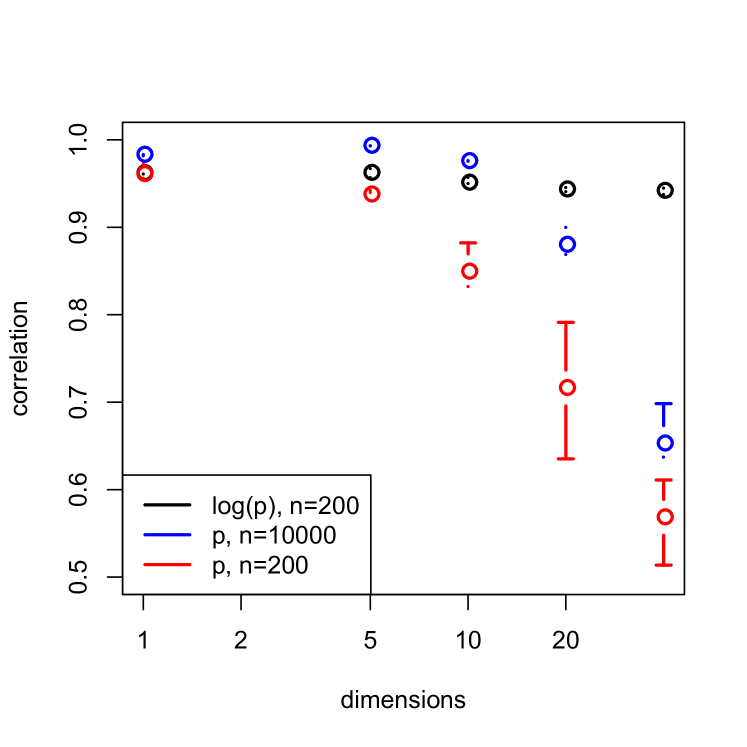
Figure 3: Estimate performance degrades in high dimensions due to over-smoothing (blue and red), but the estimator is still highly accurate up to log concentration parameter (black).

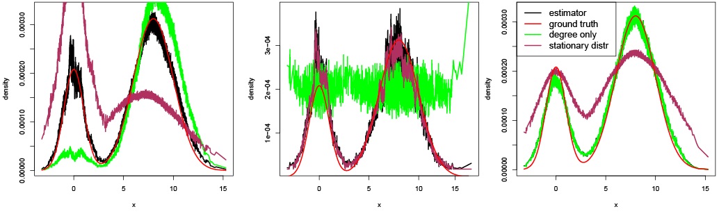
Figure 4: Example isotropic graphs. Our estimator (black) agrees with the true density (red) in all cases. Degree and stationary distribution (green and maroon) based density estimates work for some cases (right two panels) but cannot work if the degree is tied to spatial location (left).

Kernel graphs

We validate the nonparametric estimator in Corollary 4.2 for kernel graphs by constructing three drastically different kernel graphs. In all cases, we sampled 5000 points with the connection probability following $p_{i,j}=\exp(-\varepsilon(x_{i})^{-1}|x_{i}-x_{j}|)$. We varied the neighborhood structure $\varepsilon$ in three ways: a constant kernel, $\varepsilon(x_{i})\propto 1$; $k$-nearest neighbor kernel: $\varepsilon(x)\propto 1/\varepsilon_{k=100}$; and spatially varying kernel $\varepsilon(x)\propto|x|$.

In Figure 4, we find that our nonparametric estimator (black) always matches the ground truth (red). This example also shows that both the degree and the stationary distribution can be valid density estimators under certain assumptions, but only our estimator can deal with arbitrary isotropic graph construction methods without assumptions.

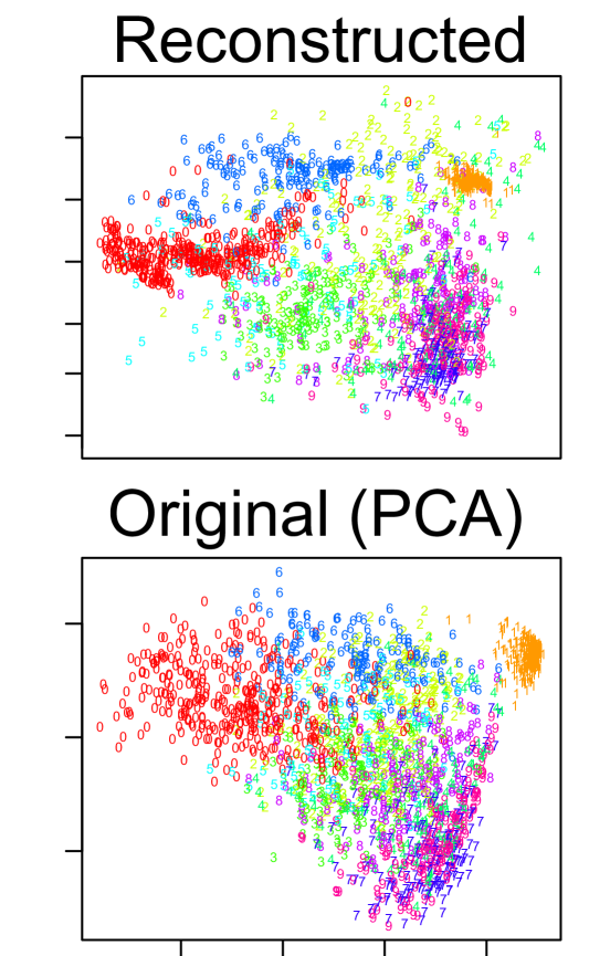
Figure 5: Reconstruction closely matches projection of the true metric.

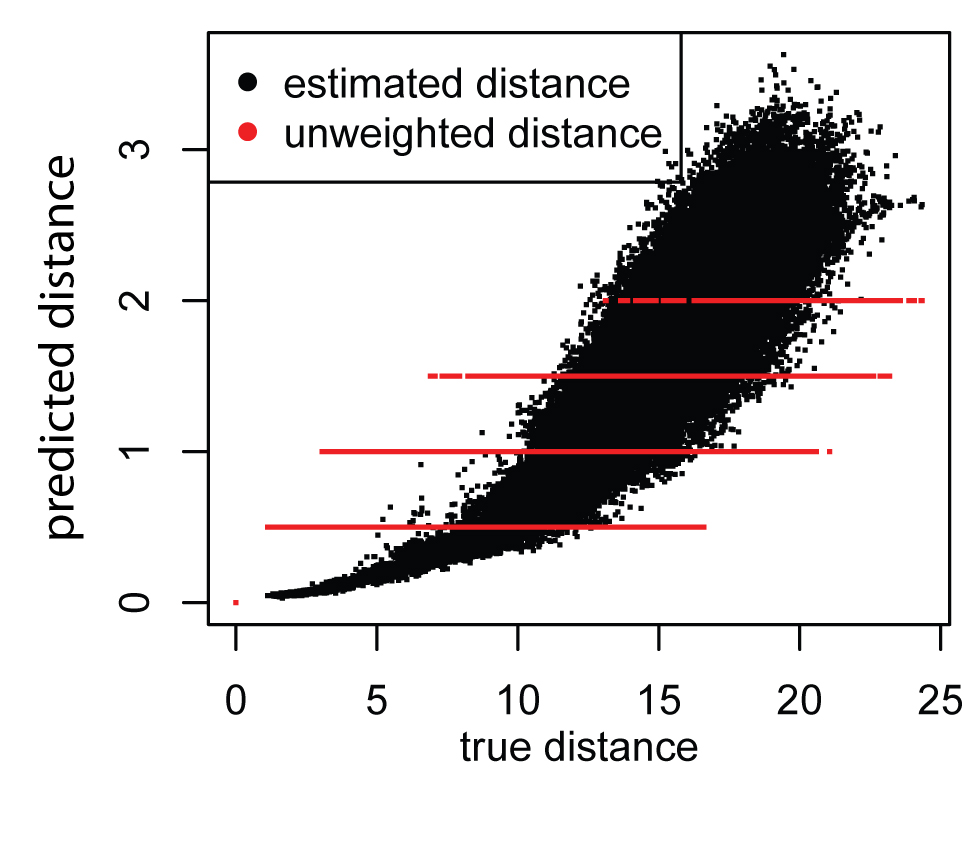
Figure 6: Distances estimated by our method are globally close to the true metric.

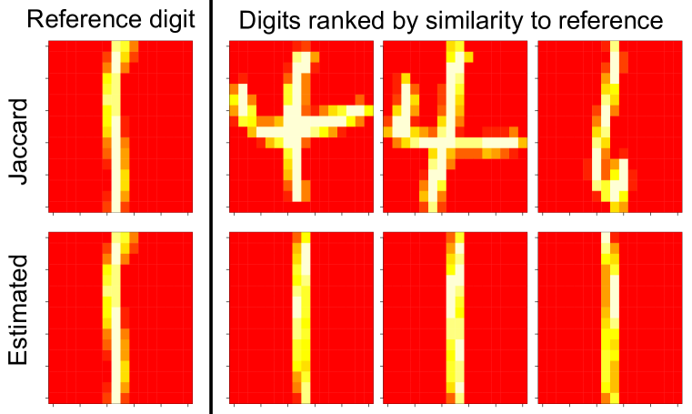
Figure 7: Items close in our weighted graph (bottom) are more similar than those under the Jaccard index (top).

Metric recovery on real data

As an example of metric reconstruction, we take the first 2000 examples in the U.S. postal service (USPS) digits dataset [7] and construct an unweighted $k$-nearest neighbor graph. We use our method to reconstruct the metric and perform similarity queries, and the Jaccard index was used to tie-break direct neighbors.

The USPS digits dataset is known to have a high-density cluster of ones digits (orange). Results in Figure 7 show that we are able to successfully recover the density structure of the data (top). Inter-point distances estimated by our method (Figure 7, $y$-axis) show nearly linear agreement to the true metric ($x$-axis) at short distances and high similarity globally.

Performing a similarity query on the data (Figure 7) shows that the our reconstructed distances (bottom row) have a more coherent set of similar digits when compared to the Jaccard index (top row) [8]. The behavior of the unweighted Jaccard similarity is due to a known problem with shortest paths in $k$-nearest neighbor graphs preferring low density regions [14].

Amazon co-purchasing data

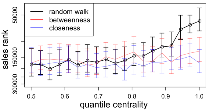
Figure 8: Density estimates in the graph correlate well with sales rank, unlike other measures of centrality.

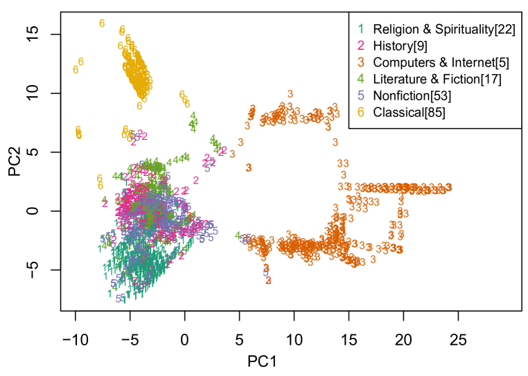
Figure 9: Embeddings from estimated distances recover the separation between different product categories.

Classics	Literature	Classical music	Philosophy
The Prince	The Stranger	Beethoven: Symphonien Nos. 5 &	The Practice of Everyday Life
The Communist Manifesto	The Myth of Sisyphus	Mozart: Symphonies Nos. 35-41	The Society of the Spectacle
The Republic	The Metamorphosis	Mozart: Violin Concertos	The Production of Space
Wealth of Nations	Heart of Darkness	Tchaikovsky: Concerto No. 1/Rac	Illuminations
On War	The Fall	Beethoven: Symphonies Nos. 3 &	Space and Place: The Perspectiv

Table 1: Top 4 clusters formed by mapping each item to its mode (first row). Each group is a coherent genre.

Finally, we recover density and metric on a real network dataset with no ground truth. We analyzed the largest connected component of the Amazon co-purchasing network dataset [9]. Each vertex is a product on amazon.com along with its category and sales rank, and each directed edge represents a co-purchasing recommendation of the form “person who bought $x$ also bought $y$.” This dataset naturally fulfills our assumptions of having edges that are asymmetric, where edges represent a notion of similarity in some space.

The items that lie in regions of highest density should be archetypal products for a category, and therefore be more popular. We show that the density estimates using our method with $d=10$ show a strong positive association between density and sales (Figure 9). We found that this effect persisted regardless of choice of $d$. Other popular measures of network centrality such as betweenness and closeness fail to display this effect.

We then attempted metric recovery using our random walk based reconstruction (Figure 9). For visualization purposes, we used multidimensional scaling on the recovered metric to embed points belonging to categories with at least two hundred items. The embedding shows that our method captures the separation across different product categories. Notably, nonfiction and history have substantial overlap as expected, while classical music CD’s and computer science books have little overlap with the other clusters.

Analyzing the modes of the density estimate by clustering each point to its local mode, we find coherent clusters where top items serve as archetypes for the cluster (Table 1). This suggests that there may be a close connection between clustering in a metric space and community detection in network data. The overall performance of our method on density estimation and metric recovery for the Amazon dataset suggests that when a metric assumption is appropriate, our random walk based metric quantities can be used directly for centrality and cluster estimates on a network.

7 Conclusions

We have presented a simple explicit identity linking the stationary distribution of a random walk on a neighborhood graph to the density and neighborhood size.

The density estimator constructed by inverting this identity shows an extremely rapid convergence to the metric $k$-nearest neighbor density estimator across a range of data point count, sparsity level, and distribution type (Figures 2,2). We also generalized the theorem to a large class of graph construction techniques and demonstrated that the choice of construction technique matters little for accuracy (Figures 4).

Our estimator performed well on real-world data, recovering underlying metric information in test data (Figures 7,7) and predicting popular Amazon products through density estimates (Figure 9).

There are several open questions left unanswered by our work. Our results required that the graphs be of degree $k=\omega(n^{2/(d+2)}\log(n)^{d/(d+2)})$ rather than the $\log(n)$ required for connectivity. Our simulation results seem to suggest than even near the $\log(n)$ regime our estimator performs nearly perfectly, suggesting that the true degree lower bound may be much lower.

The close connection of our density estimate to PageRank suggests that combining the latent spatial map with vector space estimates may lead to highly effective and theoretically principled network algorithms.

See pages - of supplement.pdf

References

- [1] M. Alamgir, G. Lugosi, and U. von Luxburg. Density-preserving quantization with application to graph downsampling. In COLT, 2014.
- [2] M. Alamgir and U. V. Luxburg. Shortest path distance in random k-nearest neighbor graphs. In Proceedings of the 29th International Conference on Machine Learning (ICML-12), pages 1031–1038, 2012.
- [3] G. Csardi and T. Nepusz. The igraph software package for complex network research. InterJournal, Complex Systems:1695, 2006.
- [4] L. P. Devroye and T. Wagner. The strong uniform consistency of nearest neighbor density estimates. The Annals of Statistics, pages 536–540, 1977.
- [5] S. N. Ethier and T. G. Kurtz. Markov processes: characterization and convergence. John Wiley & Sons, 1986.
- [6] M. Hein, J.-y. Audibert, U. V. Luxburg, and S. Dasgupta. Graph Laplacians and their convergence on random neighborhood graphs. Journal of Machine Learning Research, page 2007, 2006.
- [7] J. J. Hull. A database for handwritten text recognition research. Pattern Analysis and Machine Intelligence, IEEE Transactions on, 16(5):550–554, 1994.
- [8] P. Jaccard. Étude comparative de la distribution florale dans une portion des Alpes et des Jura. Bulletin del la Société Vaudoise des Sciences Naturelles, 37:547–579, 1901.
- [9] J. Leskovec, L. A. Adamic, and B. A. Huberman. The dynamics of viral marketing. ACM Transactions on the Web (TWEB), 1(1):5, 2007.
- [10] L. Page, S. Brin, R. Motwani, and T. Winograd. The PageRank citation ranking: Bringing order to the web. 1999.
- [11] H. Risken. Fokker-Planck Equation. Springer, 1984.
- [12] D. Stroock and S. Varadhan. Diffusion processes with boundary conditions. Communications on Pure and Applied Mathematics, 24:147–225, 1971.
- [13] D. Ting, L. Huang, and M. I. Jordan. An analysis of the convergence of graph Laplacians. In Proceedings of the 27th International Conference on Machine Learning (ICML-10), pages 1079–1086, 2010.
- [14] U. Von Luxburg and M. Alamgir. Density estimation from unweighted -nearest neighbor graphs: a roadmap. In Advances in Neural Information Processing Systems, pages 225–233. Springer, 2013.
- [15] W. Whitt. Some useful functions for functional limit theorems. Math. Oper. Res., 5(1):67–85, 1980.
- [16] W. Woess. Random walks on infinite graphs and groups - a survey on selected topics. Bull. London Math. Soc, 26:1–60, 1994.