Time-warped growth processes, with applications to the modeling of boom–bust cycles in house prices

Abstract

House price increases have been steady over much of the last 40 years, but there have been occasional declines, most notably in the recent housing bust that started around 2007, on the heels of the preceding housing bubble. We introduce a novel growth model that is motivated by time-warping models in functional data analysis and includes a nonmonotone time-warping component that allows the inclusion and description of boom–bust cycles and facilitates insights into the dynamics of asset bubbles. The underlying idea is to model longitudinal growth trajectories for house prices and other phenomena, where temporal setbacks and deflation may be encountered, by decomposing such trajectories into two components. A first component corresponds to underlying steady growth driven by inflation that anchors the observed trajectories on a simple first order linear differential equation, while a second boom–bust component is implemented as time warping. Time warping is a commonly encountered phenomenon and reflects random variation along the time axis. Our approach to time warping is more general than previous approaches by admitting the inclusion of nonmonotone warping functions. The anchoring of the trajectories on an underlying linear dynamic system also makes the time-warping component identifiable and enables straightforward estimation procedures for all model components. The application to the dynamics of housing prices as observed for 19 metropolitan areas in the U.S. from December 1998 to July 2013 reveals that the time setbacks corresponding to nonmonotone time warping vary substantially across markets and we find indications that they are related to market-specific growth rates.

, and T1Supported in part by National Science Foundation Grant DMS-10-07583. T2Supported in part by National Science Foundation Grant DMS-11-06690. T3Supported in part by National Science Foundation Grants DMS-11-04426 and DMS-12-28369.

1 Introduction

House price increases have been steady over much of the last 40 years, but there have been occasional declines, most notably in the recent housing bust that started around 2007. If underlying inflation was acting without any additional market forces, this would imply a steady rate of increase in house prices such that log prices are linearly increasing with inflation. However, asset prices typically do not follow a simple growth model with steady price increases, but rather are subject to occasional wild oscillations, as exemplified by the recent U.S. housing boom and bust cycle that led to a major worldwide financial crisis. Such asset price swings have been attributed to irrational and herd behavior of investors by Shiller, who identified and described these forces [Shiller (2005, 2008, 2013)] which render housing markets inefficient [Case and Shiller (1989)]. Shiller received a Nobel prize in economics in 2013 for this work.

It is therefore of substantial interest to determine asset price dynamics in time windows around asset bubbles, which have been a historically recurring phenomenon, in order to understand which features capture and describe the extent and dynamics of bubbles and busts, a topic that has found recurring interest [Bondt and Thaler (1985), Case and Shiller (2003), Yan, Woodard and Sornette (2012, 2014)]. The idea of an underlying smooth and stable growth trajectory in asset prices motivates a model that includes an underlying first order linear differential equation with a market-specific growth rate, which by itself reflects steady exponential growth. This component then needs to be complemented by a boom–bust component, for which we employ nonparametric time warping. The idea is that a price bust leads to a setback in time, while a boom leads to an acceleration in the way time moves forward, as prices move faster into the future than the actual flow of chronological time.

Colloquially, a setback in time when a bust occurs is reflected in statements that house or other asset prices are currently at levels that correspond to those of a past calendar year. Thus, we model longitudinal growth trajectories for house prices and other phenomena where temporal setbacks may be encountered, such as other asset prices or weight increases in growing organisms, by decomposing the observed growth into an underlying steady growth component that anchors the observed trajectories in a simple linear system, and time warping to reflect price swings. The application of our approach for asset price modeling to housing prices, as observed for 19 metropolitan areas in the U.S. from December 1998 to July 2013, reveals that the amounts of time setbacks between the markets vary substantially and are related to underlying growth features.

We view the price curves observed for various markets as a sample of functional data. Such data have become commonplace in many fields, including chemometrics, econometrics, etc. [Ferraty and Vieu (2006), Ramsay and Ramsey (2002)]. As features not only vary in terms of amplitude, but also in time of occurrence, time variability across curves is a common observation. For example, when considering biological growth, humans achieve maximum growth velocity at a subject-specific age, as subjects progress to and through puberty at different ages. Time warping (also known as registration or alignment) aims to address this variability by transforming the time domain of each function, normally under the constraint of monotonicity. Curve alignment is also motivated by the belief that for many systems, it is a (subject specific) intrinsic time, rather than clock time, that governs the underlying dynamics. In such situations, the explicit inclusion of time warping in functional data models leads to reduced variability and better interpretation. In Functional Data Analysis the presence of time warping is often considered a nuisance. In contrast, for the case of asset prices, time warping corresponds to a component reflecting price swings and bubbles and therefore is a key part of asset price modeling. In usual functional data settings, the presence of time warping routinely leads to identifiability problems, as time and amplitude variation are generally not separable in functional data settings, where one aims at modeling a sample of random functions [Kneip and Gasser (1992), Wang and Gasser (1999), Liu and Müller (2004)].

A popular approach for curve alignment is the landmark method where one defines a set of landmarks, which then are time transformed so as to occur at the same transformed time points across curves [Sakoe and Chiba (1978), Kneip and Gasser (1988)]. More recent work on curve alignment and registration includes James (2007) (curve alignment by moments), Kneip and Ramsay (2008) (alignment and functional principal components), Telesca and Inoue (2008) (Bayesian approaches to time warping), Tang and Müller (2008) (inferring global registration from pairwise warping), Sangalli et al. (2010) ($k$-means alignment for curve clustering) and Srivastava et al. (2011) (registration of functional data with the Fisher–Rao metric).

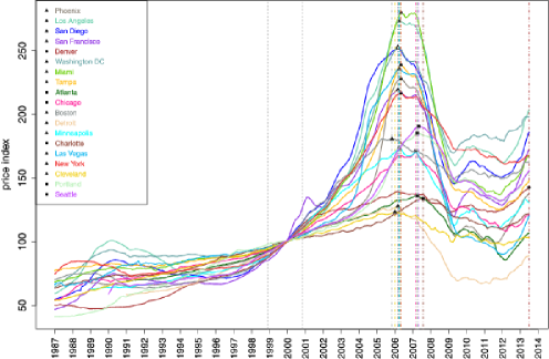
Figure 1: Housing price indices for 19 metropolitan areas in the U.S. from January 1987 to July 2013. These indices are three-month moving averages and are normalized to have a value of 100 in January 2000 (for more details, see Section 3).

Our proposed approach to time warping is more general than previous approaches in two key respects: first, it allows for inclusion of nonmonotone time-warping functions, an essential feature for modeling the busts that occur in boom–bust cycles, since these correspond to a setback in time, with prices recurring to those of a past period. Second, it overcomes the usual identifiability problems of the time-warping component by anchoring the trajectories to an underlying linear dynamic system. This anchoring makes it possible to introduce straightforward estimation procedures for all model components. While the central interest of this paper is the analysis of price oscillations in housing markets, our model extends beyond housing prices to other systems for which an underlying growth rate may be assumed, such as long-term behavior of the stock market or similar markets, for which long-term appreciation rates are meaningful [Bondt and Thaler (1985)].

As an illustration that growth may substantially deviate from an exponential trajectory (e.g., during an economic bubble) or growth may even become negative (e.g., during the burst of a bubble), Figure 1 shows seasonally adjusted S&P/Case–Shiller Home Price Indices for $19$ metropolitan areas in the United States from 1987 to 2013. As can be seen from this figure, the housing price trajectories do not correspond to exponential curves, especially after year 2000. Indeed, many areas enjoyed higher growth rates from 2000 to 2006, as compared to the 1990s. However, this accelerated growth was followed by a bust, a sharp decline of housing prices after 2006/2007.

Even though the general trends are somewhat similar across the metropolitan areas, the timing of the peak price, periods of fastest growth and rates of decline after the peak, etc., turn out to be quite variable. Coupled with the underlying linear dynamics, these variations can be accounted for by area-specific warping effects. Figures 2 and 3 show the warping functions for the time period 1998 to 2013 derived from the model proposed in Section 2. It can be seen that housing prices first warped forward in time. After the housing market collapsed around 2006/2007, the housing price warped backward in time and then started to move forward again around 2012. But for all markets except for Portland, Oregon, the warped time remains substantially below the calendar time until the present. Interestingly, these time setbacks vary quite a bit between different housing markets. The time setback of housing prices is consistent with the notion of an economic time reset, which has been featured in many discussions since the onset of the recent recession.

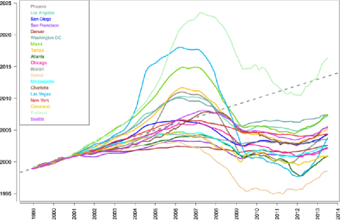
Figure 2: Warping functions for 19 metropolitan areas in the U.S. from December 1998 to July 2013. The broken grey line represents the identity function $h(t)=t$.

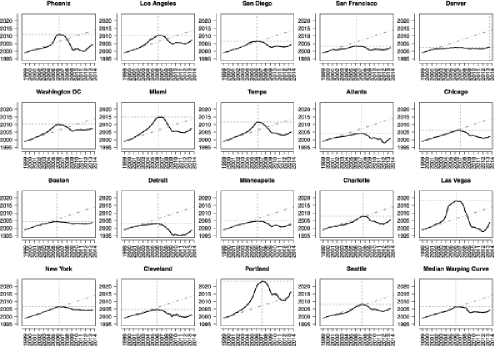
Figure 3: Time-warping functions for 19 metropolitan areas in the U.S. from December 1998 to July 2013 (drawn in individual panels), mapping chronological time (on the abscissa) to market time (ordinate). Dashed grey lines represent the identity function $h(t)=t$. Vertical grey lines indicate the timing of peak price, while horizontal grey lines indicate the level of peak price.

In addition to mapping asset price development on a market-specific timeline, our analysis and methodology identifies boom and bust components in the time-warping functions and positions the different housing markets on a boom–bust plane that indicates to what extent specific markets reflect boom or bust to a larger or lesser extent. We also explore relationships of booms and busts with underlying steady growth rates. The basic model is introduced in the next section, and a study of boom–bust cycles follows in Section 3. Our analysis is supported by simulation results that are reported in Section 4 and theoretical considerations that are in the Appendix. The paper ends with a discussion in Section 5.

2 Time-warped growth model

Our approach is to model the observed continuous time asset price trajectories through an underlying linear dynamical system, coupled with a random time-warping component. The $i$th trajectory $X_{i}(\cdot)$ that corresponds to the housing price curve of a city, as quantified by the Case–Shiller house price index, GDP per capita curve of a country or stock market index, is assumed to result from time warping due to “irrational” market forces that act in conjunction with an underlying “smooth growth” process $Z_{i}(\cdot)$ that corresponds to an underlying market-specific rate of appreciation. Scaling the observation time to $[0,1]$,

$$X_{i}(t)=Z_{i}\bigl{(}h_{i}(t)\bigr{)},\qquad t\in[0,1],i=1,\ldots,n,$$ (1)

where $h_{i}(t)$ is a market-specific warping function, a key component of our model. Furthermore, the underlying “smooth” growth process $Z_{i}(\cdot)$ that reflects market-specific long-term growth is assumed to follow a first order linear ordinary differential equation, that is,

$$Z_{i}^{\prime}(t)=\alpha_{i}Z_{i}(t),\qquad t\in[0,1],i=1,\ldots,n.$$ (2)

Here $\alpha_{i}>0$ is a market-specific random effect that captures the intrinsic growth rate of the $i$th market.

From equations (1) and (2), we have

$$X_{i}^{\prime}(t)=Z_{i}^{\prime}\bigl{(}h_{i}(t)\bigr{)}h_{i}^{\prime}(t)=\alpha_{i}Z_{i}\bigl{(}h_{i}(t)\bigr{)}h_{i}^{\prime}(t)=\alpha_{i}X_{i}(t)h_{i}^{\prime}(t),$$ (3)

whence,

$$\alpha_{i}h_{i}^{\prime}(t)=\frac{X_{i}^{\prime}(t)}{X_{i}(t)}=\frac{d}{dt}\log\bigl{(}X_{i}(t)\bigr{)}.$$

If we assume $h_{i}(0)=0$ ($i=1,\ldots,n$), then

$$h_{i}(t)=\frac{1}{\alpha_{i}}\log\frac{X_{i}(t)}{X_{i}(0)},\qquad t\in[0,1],i=1,\ldots,n.$$ (4)

As market prices $X_{i}(\cdot)$ generally tend to increase in the long term but are nonmonotonic in the shorter term (as demonstrated by the housing price trajectories in Figure 1), the warping functions $h_{i}(\cdot)$ will be nonmonotonic. Moreover, if for some $0\leq t\leq 1$, $X_{i}(t)<X_{i}(0)$, then $h_{i}(t)$ will be negative. We interpret decreasing warping functions as time moving backward, while increasing warping functions would signal time moving forward. When a warping function is negative or greater than $1$, it is interpreted as the system having warped back to the past or having leapt forward to the future beyond the time interval where the sample curves are being observed, respectively.

From equation (4), the warping function $h_{i}(\cdot)$ is determined not only by the observed process $X_{i}(\cdot)$, but also by the intrinsic growth rate $\alpha_{i}$. The model specified by equations (1) and (2) is therefore identifiable up to $\alpha_{i}h_{i}(t)$. A plausible assumption that we will make to render the model fully identifiable is that the observed trajectory $X_{i}(\cdot)$ follows a linear dynamical system on a small time interval, say, $[0,t_{0}]$, where growth is smooth, without price oscillations, so that there is no disturbance from the random warping and the warping function on this interval is $h_{i}(t)=t,t\in[0,t_{0}]$. Then we may model $X_{i}(\cdot)$ as

$$X^{\prime}_{i}(t)=\alpha_{i}X_{i}(t),\qquad t\in[0,t_{0}].$$ (5)

For example, from Figure 1, we find that the housing prices followed nearly exponential growth paths in the late 1990s/early 2000, and the growth rates $\alpha_{i}$ can then be recovered from this time interval.

Specifically, from (3), it is easy to see

$$\alpha_{i}h_{i}^{\prime}(t)=\alpha_{i},\qquad t\in[0,t_{0}],$$

so that $h_{i}(0)=0$ implies

$$h_{i}(t)=t,\qquad t\in[0,t_{0}].$$ (6)

Since on $[0,t_{0}]$, $X_{i}(t)=C\exp(\alpha_{i}t)$, $\alpha_{i}$ is determined by

$$\alpha_{i}=\frac{1}{t}\log\frac{X_{i}(t)}{X_{i}(0)},\qquad t\in(0,t_{0}]$$

or, equivalently,

$$\log X_{i}(t)=\log X_{i}(0)+\alpha_{i}t,\qquad t\in[0,t_{0}].$$ (7)

Under the model specified by (1), (2) and (5), $\alpha_{i}$ is interpreted as the rate of growth on the time period $[0,t_{0}]$ and the warping function $h_{i}(\cdot)$ captures the (possible) deviation of the system on the time period $[t_{0},1]$ from the linear dynamics on the time period $[0,t_{0}]$.

From now on, we work within the framework of this model, as we are primarily interested in identifying the patterns of the most recent housing market cycle. The time period $[0,t_{0}]$ is chosen as a two-year period in the late 1990s/early 2000s; more discussion on this choice follows below. Our goal is to study the patterns of house price oscillations during the past 10 years, contrasting it to a smooth price growth prior to this period.

In practical applications, data may not always follow the model exactly, so that equation (7) only holds approximately. Then one may obtain an underlying smooth growth rate $\alpha_{i}$ by minimizing a sum of squares type criterion,

$$\alpha_{i}=\operatorname{arg}\min_{\alpha_{i}>0}\int_{[0,t_{0}]}\bigl{(}\log X_{i}(t)-\log X_{i}(0)-a_{i}t\bigr{)}^{2}\,dt,$$ (8)

where integrals are approximated in practice by appropriate Riemannian sums. We adopted this approach for the analysis of the housing price index data in the next section, where the interval $[0,t_{0}]$ is chosen so as to maximize the coefficient of determination when fitting model (7) to the data. Another option to determine the rate $\alpha_{i}$ would be to use external information, such as a historic market rate of price appreciation, which may be tied in some way to the development of rents or inflation under the belief that the “rational” increase in house prices would match this underlying growth rate in the future [Shiller (2005)].

Note that the $\alpha_{i}$ serve as nuisance parameters and are not of interest in themselves, in contrast to the warping functions $h_{i}$, which capture the departures from the “rational” growth rate in the presence of price swings. Once growth rates $\alpha_{i}$ are obtained, by (4) one arrives at the time-warping functions

$$h_{i}(t)=\frac{1}{\alpha_{i}}\bigl{(}\log X_{i}(t)-\log X_{i}(0)\bigr{)},\qquad i=1,\ldots,n.$$ (9)

We then determine the main modes of variation of the warping functions through functional principal component analysis (FPCA). This method has evolved into a powerful tool of functional data analysis to summarize functional data and to capture their variation [Castro, Lawton and Sylvestre (1986), Rice and Silverman (1991), Ramsay and Silverman (2005), Yao, Müller and Wang (2005), Peng and Paul (2009)]. Starting with a sample of time-warping functions, this method determines eigenfunctions $\phi_{k},k\geq 1$, of the auto-covariance operator of the underlying warping process, which forms an orthonormal basis of function space, as well as the associated eigenvalues $\lambda_{k},k\geq 1$, which provide an indication of the fraction of variance that is explained by a particular eigenfunction. Additionally, one obtains the functional principal components (FPCs) $\xi_{ik}$, which are random scores that correspond to the expansion coefficients in the eigenbasis, that is, the basis formed by the eigenfunctions. The FPCs are obtained by projecting centered time-warping functions on the $k$th eigenfunction, $k\geq 1$. FPCA provides a parsimonious representation of the data and achieves efficient dimension reduction. Further details about the methodology and consistency results can be found in the Appendix.

A tool to visualize FPCA that we employ for the housing price data is the modes of variation plot [Jones and Rice (1992)]. In these plots the direction in function space, into which a given eigenfunction points, is visualized by $\mu(t)+\gamma\sqrt{\lambda}_{k}\phi_{k}(t),t\in[0,1]$, where one varies $\gamma$ over a range of values, typically $\gamma\in[-2,2]$. This plot provides a visual indication of the movement from the mean function $\mu$ toward the positive and negative direction of the $k$th eigenfunction $\phi_{k}$.

3 Boom and bust in U.S. housing markets

Here, we apply the method described in Section 2 to study the housing price trends in 19 U.S. metropolitan areas. The data were downloaded from http://www.spindices.com/index-family/real-estate/sp-case-shiller. The original data consist of seasonally adjusted Case–Shiller Home Price Indices [Case and Shiller (1987)] for each month for 20 metropolitan areas and two composite indices from January 1987 to July 2013. These indices are three-month moving averages and are normalized to have a value of $100$ in January 2000. For more details about how the housing indices are calculated, see “S&P/Case–Shiller Home Price Indices Methodology” published by Standard & Poor’s. Since for Dallas, Texas, housing price indices are only available after 2000, we drop it from our analysis and thus focus on the remaining $19$ metropolitan areas.

The housing price index trajectories for these 19 areas are depicted in Figure 1. For some areas, there is a clear bubble in the housing market after year 2000, in the sense that housing prices increased super-exponentially. This phenomenon is clearly illustrated by the warping functions depicted in Figure 3. Also, the timing of the “peak price” (indicated by the dashed colored lines in Figure 1) is mainly clustered into two groups: a larger group of $13$ areas (triangles) where peak price occurred around late 2005 and early 2006, and a smaller group of $5$ areas (squares) where peak price occurred around the first two quarters of 2007. The only exception is Denver, Colorado (diamond), where the summer 2013 indices are slightly higher than the pre-recession peak that occurred in Febuary/March, 2006.

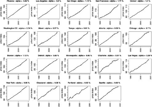
Figure 4: Exponential fit (broken grey lines) of housing price indices (solid lines) between December 1998 and November 2000, where the $\alpha_{i}$ are expressed as $\%$ per month.

We then fitted exponential curves to all 2-year, 3-year, 5-year time intervals within 1991 to 2013 (we started from 1991 since there is no missing data after that) and found that for the 2-year interval from December 1998 to November 2000 (the period between the two dotted grey lines on Figure 1), the exponential fits result in the largest overall coefficient of determination $R^{2}$. As can be seen from Figure 4, the exponential curve fits the housing price trajectory between December 1998 and November 2000 very well. More specifically, on this interval, among the fits for these $19$ markets, the smallest $R^{2}$ is $0.967$ (Charlotte) and the largest $R^{2}$ is $0.998$ (Denver). Since our major interest is in investigating the boom–bust cycles of the housing market in recent years, we choose December $1998$ as our starting time. Specifically, we treat December 1998 as time $0$, and July 2013 as time $1$ in the normalized time scale. We also elect $t_{0}$ to correspond to November 2000 and use $[0,t_{0}]$ to estimate the growth rates $\alpha_{i}$ by equation (8). The average growth rate of these $19$ metropolitan areas is 0.75% per month, with a standard deviation of $0.37\%$ per month.

It can be seen that some markets, including San Diego, San Francisco, Denver, Boston, Minneapolis and New York, already had a fast growth rate at the end of the last century (with an $\alpha_{i}$ around or above $1\%$ per month). Figure 3 shows the warping function for each area defined by equation (9), as well as the median warping curve across these 19 markets (in the last panel). One finds that the markets already growing fast at the end of the last century mostly retained a similar growth rate after 2000 until the housing market collapsed around 2006/2007. Some markets, including Washington DC, Miami, Tampa, Las Vegas and Portland, went through a much faster price growth period after 2000. The housing price trend of Detroit is quite unique. This market had moderate growth at the end of last century ($\alpha_{i}=0.65\%$), followed by declines toward 2000 and a sharp drop after 2006, which places it in a separate category from the rest.

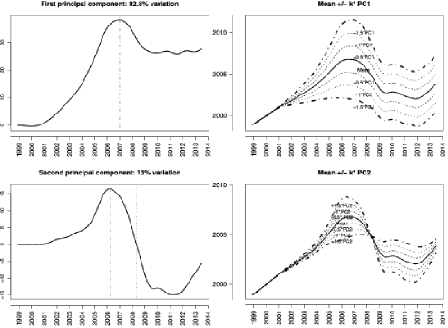
Figure 5: First two eigenfunctions (multiplied by the square-root of their respective eigenvalues) of the time-warping process.

We then apply FPCA for the warping functions, as described in Section 2. The first two principal components explain $\sim 96\%$ of the total variation in the warping functions. However, Las Vegas and Portland appear to be outliers. In order to avoid the influence of these outliers on our analysis, we dropped Las Vegas and Portland and redid the FPCA for the remaining $17$ markets. Again, the first two principal components explain nearly $96\%$ of the total variation (1st PC: $82.8\%$, 2nd PC $13\%$). Figure 5 shows the first two eigenfunctions (multiplied by the square-root of their respective eigenvalues), which display some remarkable features. First, the first eigenfunction has a shape that is similar to that of the mean function. This means a large fraction of the variance is explained by what amounts roughly to the degree at which the average boom cycle is expressed. Second, the first eigenfunction primarily reflects the rise of the house price to a high peak (around December, 2006) in the boom cycle and the subsequent fall, but to a level that is still substantially higher than the 2000 price level. Thus, this component primarily reflects the boom part of the cycle and is referred to as the “boom” component. Third, the second eigenfunction features an earlier (around March, 2006), smaller but steeper peak, and then a deep fall to a very low level. Thus, this component primarily reflects the bust part of the cycle and we call it the “bust” component. It is also interesting to note that the second eigenfunction went from positive to negative in early $2008$, which coincides with the onset of the economic recession.

Figure 6: First two principal component scores of $17$ metropolitan areas in the U.S.

Although the estimation of the growth rates $\alpha_{i}$ may change when the fitting interval, on which exponential growth is assumed, varies, we found that the FPCA results do not depend much on the choice of the fitting interval. When we applied the fitting procedure for the $\alpha_{i}$ on a different two-year interval, namely, January 1998 to December 1999, the resulting eigenfunctions have almost identical shapes: the two leading principal components explain the majority of the variation in the data, and the first component represents a boom component and the second component corresponds to a bust component. For more details, see the supplementary material [Peng, Paul and Müller (2014)].

After extracting the first and second functional principal components (which are the scalar random variables that are multiplied with the eigenfunctions in the representation of the time-warping functions), we plot the “bust” component against the “boom” component in Figure 6. The markets falling in the right lower quadrant (e.g., Washington, DC) experienced a boom but relatively little bust, while those in the right upper quadrant (e.g., Miami) experienced both boom and bust in similar measure. The areas in the left upper quadrant have been subject to a bust with little boom (e.g., Detroit), while those in the lower left quadrant had little boom or bust (e.g., Denver). Even though Las Vegas and Portland have not been used to derive these components, their projected first two PC scores are $1.65$ and $5.57$ for Las Vegas and $4.82$ and $-$0.39 for Portland. This indicates that in the boom–bust coordinates that emerged from the FPCA, Las Vegas experienced a big housing boom, followed by an enormous bust, while Portland enjoyed a huge boom with little bust.

Also of interest are relations between the time-warping functions, as characterized by their first two principal component scores, which serve as random effects in the eigen-expansion (see the Appendix for more details) and the underlying growth rate $\alpha_{i}$, which may be viewed as a market-specific characteristic. The corresponding scatterplots of first (resp., second) principal component score versus $\alpha_{i}$ with the superimposed least squares line in Figure 7 demonstrate that regions with lower baseline growth rates experienced stronger boom–bust cycles. The relationship seems particularly striking for the bust component.

Figure 7: Principal component scores versus growth rate $\alpha_{i}$.

4 Simulation results

In this section we report a simulation experiment that was conducted to investigate the practical performance of the proposed procedure. This simulation was designed to mimic the housing index data, and $n$ warping functions were generated as

$$h_{i}(t)=\mu(t)+\sum_{k=1}^{K}\sqrt{\lambda_{k}}\xi_{ik}\phi_{k}(t),\qquad t\in[T_{0},T_{1}],i=1,\ldots,n.$$

The sample size was chosen as $n=20$, the mean function $\mu(\cdot)$ was chosen as the estimated mean warping function of the housing data (solid curve in the upper-right panel of Figure 5), $K=10$ and $\{\phi_{k}(\cdot)\}_{k=1}^{10}$ were chosen as the first $10$ eigenfunctions estimated from the housing data (upper-left and lower-left panels of Figure 5 show the first two eigenfunctions), furthermore, the eigenvalues $\{\lambda_{k}\}_{k=1}^{10}$ were chosen to correspond to those in the housing price analysis, and the functional principal component scores $\xi_{ik}$ were chosen as i.i.d. from $N(0,1)$. The time interval is set as $T_{0}=144$ and $T_{1}=319$, reflecting the monthly indices from December 1998 to July 2013, respectively (January 1987 is month $1$).

We then generated the price trajectories according to equation (4), namely,

$$X_{i}(t)=X_{i}(T_{0})\exp\bigl{\{}\alpha_{i}\bigl{(}h_{i}(t)-h_{i}(T_{0})\bigr{)}\bigr{\}},\qquad t\in[T_{0},T_{1}],i=1,\ldots,n,$$

where the initial values $X_{i}(T_{0})$ were chosen as i.i.d. from $\operatorname{Uniform}(85,100)$, while the growth rates $\alpha_{i}$ were randomly generated from $\operatorname{Uniform}(0.003,\break 0.018)$, where only samples that satisfied the boundedness condition$\max_{t\in[T_{0},T_{1}]}X_{i}(t)<300$ were retained. The interval (85,100) is set according to the range that was observed for the housing indices in December 1998, while the interval $(0.003,0.018)$ matches the range of the estimated $\alpha_{i}$ from the housing data. The trajectories are capped at $300$ since the maximum index in the housing data is $280$.

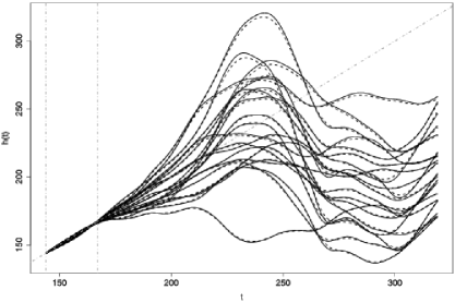
Figure 8: Simulated warping functions: true—solid lines, estimated—broken lines. The dashed grey line represents the identity function $h(t)=t$. Vertical grey lines indicate the end points of the fitting region for the growth rates used in the real data, namely, December 1998 (month 144) and November 2000 (month 167).

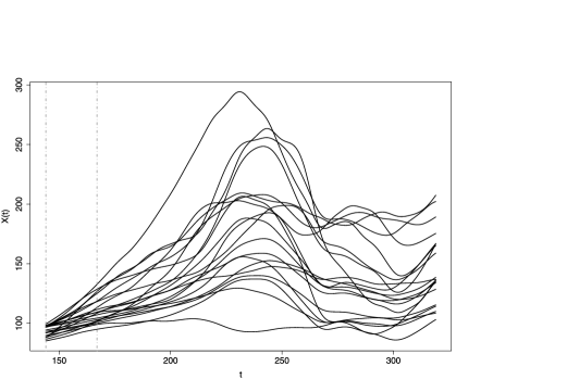
Figure 9: Simulated price trajectories. Vertical grey lines indicate the end points of the fitting region for the growth rates used in the real data, namely, December 1998 (month 144) and November 2000 (month 167).

Figure 8 shows $20$ simulated warping functions (solid lines) and Figure 9 shows the corresponding simulated price trajectories. The two vertical grey lines in these figures indicate the end points of the fitting region for the growth rates used in the real data, namely, December 1998 (month $144$) and November 2000 (month $167$).

We then applied the same procedures used for analyzing the housing price index data. First, we fitted exponential curves on all 24-month, 36-month and 60-month time intervals and calculated the coefficient of determination $R^{2}$ for each market on each of these intervals. We picked the interval corresponding to the largest averaged $R^{2}$ (across the $20$ subjects). For the data in Figure 9, the best interval coincides with the fitting region used in the real data. The corresponding averaged $R^{2}$ is $0.997$ and the estimated $\alpha_{i}$ have an averaged relative squared error (ASE) $\frac{1}{n}\sum_{i=1}^{n}\frac{(\hat{\alpha}_{i}-\alpha_{i})^{2}}{\alpha_{i}^{2}}$ of $9.51\times 10^{-5}$. The warping functions were estimated as described in Section 2 [equation (9)], and these estimates are displayed as broken lines in Figure 8. FPCA is then applied to the estimated warping functions, and one ends up with an estimate of the eigencomponents, which are the eigenfunctions and the functional principal components; see the Appendix for a more detailed description.

We repeated the above process (including data generation and fitting) $100$ times. Across the $100$ replicates, the ASE for estimating the $\alpha_{i}$ had a mean of $0.011$ and a standard deviation of $0.041$. The left end point of the $\alpha$ fitting region was found to have a mean of $146.31$ and a standard deviation of $7.58$, while the right end point had mean $169.43$ with standard deviation $7.93$. The mean relative-integrated-squared-error for the warping function estimation was $0.032$.

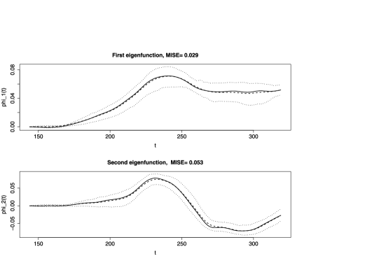
Figure 10: First two simulated eigenfunctions: true—solid line, pointwise mean—broken line, pointwise $95\%$ and $5\%$ bands—dotted lines.

Figure 10 shows the pointwise mean estimated eigenfunctions (broken lines) and the $95\%$ and $5\%$ pointwise bands (dotted lines). The mean-integrated-squared-error (MISE), namely, the average of $\|\hat{\phi}-\phi\|^{2}$ across the $100$ replicates, is $0.029$ for the first eigenfunction and $0.053$ for the second eigenfunction. The mean relative-squared-error of the first two eigenvalues are $0.825$ and $0.135$, respectively. The percentage of variation explained by the first two estimated eigenfunctions ranges from $85.5\%$ to $98.8\%$ with a mean $96\%$.

These results show that the proposed procedure is able to select the right fitting region for the growth rate $\alpha$ and that it is also effective in estimating both $\alpha$ and the warping function $h(\cdot)$. Most importantly, as can be seen from Figure 10, there is little bias in the estimation of the leading eigenfunctions. It is particularly noteworthy that the estimators are able to preserve the shape of the eigenfunctions (as reflected by the two bands).

5 Discussion

In this paper we introduce a new model for asset price modeling that is motivated by and illustrated with the recent price swings observed in the U.S. real estate market. Introducing an interface between an underlying dynamic “steady growth” model and time warping leads to interesting results and insights about asset price dynamics. Our approach aims to model asset prices in terms of a smooth component that corresponds to a market-specific steady rate of appreciation and an oscillation component that reflects “irrational” swings in prices and their extreme manifestation in the form of boom–bust cycles, as recently experienced across the U.S. housing markets. Our analysis and modeling is not limited to real estate price dynamics and will be of interest also for the modeling of other asset prices that involve price swings and boom–bust cycles; this includes equity and art markets.

Key findings from our analysis are that for the recently burst bubble in U.S. house prices across several metropolitan area markets, one can clearly distinguish a boom component and a bust component, which are characterized by the shapes of the first (boom) and second (bust) eigenfunctions. The functional principal components that correspond to the strength of boom and bust, respectively, are uncorrelated (Figure 6). Thus, the price swings observed over the last 15 years can be classified into four distinct categories, markets that exhibited primarily a bust component (Detroit) and that are contrasted with markets with primarily a boom (Washington, DC) and, on the other hand, markets that experienced a combined strong boom and bust cycle (Miami) and those with relatively weaker booms and busts (Denver). The latter is likely due to these market’s strong underlying growth rates. This means that a bust phase cannot be clearly predicted from the strength of a preceding boom in our quantification, and therefore is hard to predict not only in its timing but also in terms of whether it will happen or not. There are also a few “middle of the road” markets where the observed time warping is close to the overall mean time warping, which includes Chicago, San Diego and Minneapolis.

Our analysis also provides some indication that the strengths of booms and busts may be related to the underlying “rational” steady rate of growth, in the sense that lower underlying growth rates are associated with larger bust components and likely also with larger booms (Figure 7). Such relationships might reflect the preferences of investors, who primarily may have invested in the slower-growing markets, where larger subsequent booms and thus profits seemed plausible. Such an influx of investors would first drive prices up and then down when the investors leave these markets.

A central feature of our approach to analyze asset price dynamics is the new concept of nonmonotone warping functions. All existing time-warping approaches are based on monotonic warping functions, satisfying the constraint that time always flows forward. A primary motivation of requiring monotonicity is to preserve the order of events (such as landmarks). For our approach the emphasis, however, is not to preserve the forward flow of time, but rather to allow for reversals of time during periods of price deflation, implementing the notion that in such periods prices retreat to those of an earlier time.

For the existing warping approaches, difficulties arise from the fact that the warping function and the amplitude function usually are not jointly identifiable. Traditionally, this problem has been addressed by imposing a variety of identifiability constraints [Gervini and Gasser (2005), Kneip and Ramsay (2008)], none of which is particularly well motivated. Such constraints are usually imposed for technical reasons, are hard to verify and may lead to difficulties in interpreting the results. In the proposed approach, we bypass the identifiability issue through explicitly exploiting the dependency of the warping function on the observations. This requires the presence of an undisturbed interval, on which market price can be reasonably assumed to follow a simple smooth trajectory. Both the actual housing data analysis and simulations show that the choice of such an interval is not critical. The resulting warping functions are viewed here as a mechanism that gives rise to complex features and oscillations in the asset price curves through phase variation in the underlying dynamics (we assume a simple linear dynamical system).

Unlike most existing methods, the warping functions in our approach are not constrained. Particularly, they are not required to be monotonic. When a warping function is decreasing, we interpret this as a reverse time effect, that is, the corresponding system is going backward in time, while periods with increasing warping functions correspond to phases where the system is going forward in time. We emphasize that curve alignment is not our goal and, therefore, warping function monotonicity is not an issue. Rather, the warping functions themselves are objects of interest since they serve to quantify the deviations from smoothly increasing asset prices.

The assumption of an underlying linear dynamical system seems reasonable for asset price modeling. This assumption can be fairly easily replaced by another form of underlying (nonlinear of known shape) dynamical system and the results can be extended to such more general cases. The system (linear or more complex) will be fitted on a relatively undisturbed interval, where one may reasonably assume that price oscillations are absent or are minimal. We need to assume that such a period of time exists, but a priori knowledge of its exact location is not required, as the simulations clearly show.

While for the housing index data the simple linear dynamics has great appeal and provides many insights into the dynamics, it can be occasionally of interest for other applications such as demography or biological weight growth to consider an extension of our assumption that the growth rates $\alpha_{i}$ do not depend on time or age $t$. To check whether indeed this may be the case in such applications, one may consider a second (or higher) order dynamic system. If, for example, as before, $X(t)=Z(h(t))$ but now $Z^{\prime}(t)/Z(t)=\alpha(t)$, then it is easy to see that

$$\frac{X^{\prime\prime}(t)}{X(t)}=h^{\prime}(t)^{2}\bigl{[}\alpha^{\prime}\bigl{(}h(t)\bigr{)}+\alpha^{2}\bigl{(}h(t)\bigr{)}\bigr{]}+h^{\prime\prime}(t)\alpha\bigl{(}h(t)\bigr{)},$$

which can be alternatively expressed as

$$\frac{d}{dt}\frac{X^{\prime}(t)}{X(t)}=h^{\prime\prime}(t)\alpha\bigl{(}h(t)\bigr{)}+h^{\prime}(t)^{2}\alpha^{\prime}\bigl{(}h(t)\bigr{)}.$$

Such relationships can be used as a diagnostic, by first fitting the original model and then checking whether indeed $\frac{d}{dt}\frac{X^{\prime}(t)}{X(t)}=h^{\prime\prime}(t)\alpha$ as being implied by the original model.

Since the rate parameters $\alpha_{i}$ of the underlying linear dynamic systems are market-specific and thus differ across the observed curves, they provide a complete description of the smooth price increases that are complemented by the time warping. Here the baseline growth trajectories $\exp(\alpha_{i}t)$ themselves correspond to the “aligned curves,” which are thus characterized by one random growth rate. The signal of interest that relates to the “irrational” price swings is in the time warping functions and, accordingly, their functional principal component analysis characterizes the main features of interest, the modes of variation, which are of special interest for the recent boom–bust cycle of the housing markets, as we have demonstrated with the housing price analysis. Another interesting application is to combine time warping with clustering of (sub-)metropolitan areas. This may be achieved through clustering of the PC scores of warping functions as estimated in this paper. Moreover, specific features of time-warping functions $h_{i}$ can be more generally used for clustering, for example, Liu and Yang (2009), Claeskens, Hubert and Slaets (2010), Tang and Müller (2009). Such time clustering will be of interest for the analysis of housing markets, either entire metropolitan markets or sub-metropolitan areas within such markets, depending on data availability.

Appendix: Details on functional principal component analysis

In the following the warping functions $h_{i},i=1,\ldots,n$, that are derived from equation (9), are considered to be an i.i.d. sample of an underlying time-warping process $H$, defined on the interval $[0,1]$. For the functional principal component representation of the process $H$, the key components are the mean function $\mu(t)=E(H(t)),t\in[0,1]$, and the auto-covariance function $G(s,t)=\operatorname{cov}(H(s),H(t)),s,t\in[0,1]$.

We assume throughout that the time-warping process $H$ has smooth and square integrable trajectories, $E\int_{[0,1]}H^{2}(t)\,dt<\infty$. Then the eigenfunctions $\phi_{k},k\geq 1$, of the auto-covariance operator $A(f)(t)=\int_{[0,1]}f(s)G(s,t)\,ds,t\in[0,1]$, which is a linear Hilbert–Schmidt operator that maps $L^{2}([0,1])$ into itself, form the orthonormal eigenbasis. Processes $H$ may then be represented in this basis by means of the Karhunen–Loève expansion [Ash and Gardner (1975)]

$$H(t)=\mu(t)+\sum_{k\geq 1}\xi_{k}\sqrt{\lambda}_{k}\phi_{k}(t),\qquad t\in[0,1],$$

where the $\xi_{k}\sqrt{\lambda}_{k}$ are the functional principal components, which correspond to projections $\xi_{k}\sqrt{\lambda}_{k}=\int_{[0,1]}(H(t)-\mu(t))\phi_{k}(t)\,dt$, and satisfy $E(\xi_{k})=0$ and $E(\xi_{k}^{2})=1$, with $\lambda_{k}$ denoting the $k$th eigenvalue. In the following, the $L^{2}$ norm of a function $f$ will be denoted by $\|f\|_{L^{2}}=[\int_{[0,1]}f^{2}(t)\,dt]^{1/2}$ or $\|f\|_{L^{2}}=[\int_{[0,1]}\int_{[0,1]}f^{2}(s,t)\,ds\,dt]^{1/2}$.

The empirical estimates of the mean and auto-covariance functions of $H$ are

$$\hat{\mu}(t) = \frac{1}{n}\sum_{i=1}^{n}h_{i}(t),\qquad t\in[0,1],$$ (10)

$$\hat{G}(s,t) = \frac{1}{n}\sum_{i=1}^{n}h_{i}(s)h_{i}(t)-\hat{\mu}(s)\hat{\mu}(t),\qquad s,t\in[0,1].$$ (11)

From the fact that $E(\hat{\mu})=\mu$ and the square integrability, one immediately finds $E\|\hat{\mu}-\mu\|_{L^{2}}^{2}=\frac{1}{n}\int_{[0,1]}\operatorname{var}(H(t))\,dt$ and, therefore, $\|\hat{\mu}-\mu\|_{L^{2}}=O_{p}(n^{-1/2})$. Using more intricate arguments, it can been shown that under the additional assumption that $E\|H^{2}\|_{L^{2}}^{2}<\infty$, it also holds that $\|\hat{G}-G\|_{L^{2}}=O_{p}(n^{-1/2})$ [Dauxois, Pousse and Romain (1982), Hall and Hosseini-Nasab (2006)]. Results of the above type for $\hat{\mu}$ and $\hat{G}$ are then typically coupled with a perturbation result that relates differences in eigenfunctions and eigenvalues to those of $L^{2}$ distances of covariances; an example is Lemma 4.3 in Bosq (2000), which is utilized to prove the following more rigorous results about the convergence in sup norm of the eigenfunctions and eigenvalues of the time-warping process $H$.

Such results can be obtained by adopting an approach of Chen and Müller (2012) that utilizes techniques developed in Li and Hsing (2010). Technical assumptions needed are as follows: For arbitrary universal constants $0<B<C<\infty$, it holds that for all $t$ that $E|H(t)|^{\ell}\leq\frac{\ell!}{2}C^{\ell-2}B^{2},\ell=2,3,\dots$ and for all $s,t$ that $E|H(s)H(t)|^{\ell}\leq\frac{\ell!}{2}C^{\ell-2}B^{2},\ell=2,3,\dots.$ In addition, all trajectories of $H$ are assumed to satisfy $|H(s)-H(t)|\leq C|s-t|$and $E(\sup_{t\in\mathcal{T}}|H(t)|)<\infty$, $\sup_{t\in[0,1]}|\mu(t)|<\infty$, $\sup_{s,t}|G(s,t)|<\infty$,$\sup_{t\in[0,1]}|\phi_{k}(t)|<\infty$ for each $k\geq 1$.

Under these assumptions, using similar arguments, such as those provided in Lemma 1 and Theorem 1 of Chen and Müller (2012), leads to the following consistency results:

$$\sup_{t\in\mathcal{T}}\bigl{|}\hat{\mu}(t)-\mu(t)\bigr{|} = O\bigl{(}(\log n/n)^{1/2}\bigr{)}\qquad\mbox{a.s.},$$

$$\sup_{s,t\in\mathcal{T}}\bigl{|}\hat{G}(s,t)-G(s,t)\bigr{|} = O\bigl{(}(\log n/n)^{1/2}\bigr{)}\qquad\mbox{a.s.},$$

$$\sup_{t\in\mathcal{T}}\bigl{|}\hat{\phi_{k}}(t)-\phi_{k}(t)\bigr{|} = O\bigl{(}(\log n/n)^{1/2}\bigr{)}\qquad\mbox{a.s.},$$

$$|\hat{\lambda}_{k}-\lambda_{k}| = O\bigl{(}(\log n/n)^{1/2}\bigr{)}\qquad\mbox{a.s.}$$

Here $\hat{\phi}_{k}$ and $\hat{\lambda}_{k}$ are the eigenfunction/eigenvalue estimates that one obtains from a spectral decomposition of the empirical covariance function $\hat{G}$ in (11). This is numerically implemented through suitable discretization and using matrix eigenanalysis. We note that the consistency of the estimates $\xi_{ik}\sqrt{\lambda}_{k}=\int_{[0,1]}(h_{i}(t)-\hat{\mu}(t))\hat{\phi}_{k}(t))\,dt$ of the $k$th principal components $\xi_{ik}\sqrt{\lambda}_{k},i=1,\ldots,n,k\geq 1$, follows immediately from these results.

References

- Ash and Gardner (1975) {bbook}[mr] \bauthor\bsnmAsh, \bfnmRobert B.\binitsR. B. and \bauthor\bsnmGardner, \bfnmMelvin F.\binitsM. F. (\byear1975). \btitleTopics in Stochastic Processes. \bseriesProbability and Mathematical Statistics \bvolume27. \bpublisherAcademic Press, \blocationNew York. \bidmr=0448463 \bptokimsref\endbibitem
- Bondt and Thaler (1985) {barticle}[auto:STB—2014/02/12—14:17:21] \bauthor\bsnmBondt, \bfnmW. F.\binitsW. F. and \bauthor\bsnmThaler, \bfnmR.\binitsR. (\byear1985). \btitleDoes the stock market overreact? \bjournalJ. Finance \bvolume40 \bpages793–805. \bptokimsref\endbibitem
- Bosq (2000) {bbook}[mr] \bauthor\bsnmBosq, \bfnmD.\binitsD. (\byear2000). \btitleLinear Processes in Function Spaces: Theory and Applications. \bseriesLecture Notes in Statistics \bvolume149. \bpublisherSpringer, \blocationNew York. \biddoi=10.1007/978-1-4612-1154-9, mr=1783138 \bptokimsref\endbibitem
- Case and Shiller (1987) {bmisc}[auto:STB—2014/02/12—14:17:21] \bauthor\bsnmCase, \bfnmK. E.\binitsK. E. and \bauthor\bsnmShiller, \bfnmR. J.\binitsR. J. (\byear1987). \bhowpublishedPrices of single family homes since 1970: New indexes for four cities. Unpublished manuscript. \bptokimsref\endbibitem
- Case and Shiller (1989) {barticle}[auto:STB—2014/02/12—14:17:21] \bauthor\bsnmCase, \bfnmK. E.\binitsK. E. and \bauthor\bsnmShiller, \bfnmR. J.\binitsR. J. (\byear1989). \btitleThe efficiency of the market for single-family homes. \bjournalAm. Econ. Rev. \bvolume79 \bpages125–137. \bptokimsref\endbibitem
- Case and Shiller (2003) {barticle}[auto:STB—2014/02/12—14:17:21] \bauthor\bsnmCase, \bfnmK. E.\binitsK. E. and \bauthor\bsnmShiller, \bfnmR. J.\binitsR. J. (\byear2003). \btitleIs there a bubble in the housing market? \bjournalBrookings Pap. Econ. Act. \bvolume2003 \bpages299–362. \bptokimsref\endbibitem
- Castro, Lawton and Sylvestre (1986) {barticle}[auto:STB—2014/02/12—14:17:21] \bauthor\bsnmCastro, \bfnmP. E.\binitsP. E., \bauthor\bsnmLawton, \bfnmW. H.\binitsW. H. and \bauthor\bsnmSylvestre, \bfnmE. A.\binitsE. A. (\byear1986). \btitlePrincipal modes of variation for processes with continuous sample curves. \bjournalTechnometrics \bvolume28 \bpages329–337. \bptokimsref\endbibitem
- Chen and Müller (2012) {barticle}[mr] \bauthor\bsnmChen, \bfnmKehui\binitsK. and \bauthor\bsnmMüller, \bfnmHans-Georg\binitsH.-G. (\byear2012). \btitleModeling repeated functional observations. \bjournalJ. Amer. Statist. Assoc. \bvolume107 \bpages1599–1609. \biddoi=10.1080/01621459.2012.734196, issn=0162-1459, mr=3036419 \bptokimsref\endbibitem
- Claeskens, Hubert and Slaets (2010) {bmisc}[auto:STB—2014/02/12—14:17:21] \bauthor\bsnmClaeskens, \bfnmG.\binitsG., \bauthor\bsnmHubert, \bfnmM.\binitsM. and \bauthor\bsnmSlaets, \bfnmL.\binitsL. (\byear2010). \bhowpublishedPhase and amplitude-based clustering for functional data. FBE Research report KBI_1030, pages 1–25. \bptokimsref\endbibitem
- Dauxois, Pousse and Romain (1982) {barticle}[mr] \bauthor\bsnmDauxois, \bfnmJ.\binitsJ., \bauthor\bsnmPousse, \bfnmA.\binitsA. and \bauthor\bsnmRomain, \bfnmY.\binitsY. (\byear1982). \btitleAsymptotic theory for the principal component analysis of a vector random function: Some applications to statistical inference. \bjournalJ. Multivariate Anal. \bvolume12 \bpages136–154. \biddoi=10.1016/0047-259X(82)90088-4, issn=0047-259X, mr=0650934 \bptokimsref\endbibitem
- Ferraty and Vieu (2006) {bbook}[mr] \bauthor\bsnmFerraty, \bfnmFrédéric\binitsF. and \bauthor\bsnmVieu, \bfnmPhilippe\binitsP. (\byear2006). \btitleNonparametric Functional Data Analysis: Theory and Practice. \bpublisherSpringer, \blocationNew York. \bidmr=2229687 \bptokimsref\endbibitem
- Gervini and Gasser (2005) {barticle}[mr] \bauthor\bsnmGervini, \bfnmDaniel\binitsD. and \bauthor\bsnmGasser, \bfnmTheo\binitsT. (\byear2005). \btitleNonparametric maximum likelihood estimation of the structural mean of a sample of curves. \bjournalBiometrika \bvolume92 \bpages801–820. \biddoi=10.1093/biomet/92.4.801, issn=0006-3444, mr=2234187 \bptokimsref\endbibitem
- Hall and Hosseini-Nasab (2006) {barticle}[mr] \bauthor\bsnmHall, \bfnmPeter\binitsP. and \bauthor\bsnmHosseini-Nasab, \bfnmMohammad\binitsM. (\byear2006). \btitleOn properties of functional principal components analysis. \bjournalJ. R. Stat. Soc. Ser. B Stat. Methodol. \bvolume68 \bpages109–126. \biddoi=10.1111/j.1467-9868.2005.00535.x, issn=1369-7412, mr=2212577 \bptokimsref\endbibitem
- James (2007) {barticle}[mr] \bauthor\bsnmJames, \bfnmGareth M.\binitsG. M. (\byear2007). \btitleCurve alignment by moments. \bjournalAnn. Appl. Stat. \bvolume1 \bpages480–501. \biddoi=10.1214/07-AOAS127, issn=1932-6157, mr=2415744 \bptokimsref\endbibitem
- Jones and Rice (1992) {barticle}[auto:STB—2014/02/12—14:17:21] \bauthor\bsnmJones, \bfnmM. C.\binitsM. C. and \bauthor\bsnmRice, \bfnmJ. A.\binitsJ. A. (\byear1992). \btitleDisplaying the important features of large collections of similar curves. \bjournalAmer. Statist. \bvolume46 \bpages140–145. \bptokimsref\endbibitem
- Kneip and Gasser (1988) {barticle}[mr] \bauthor\bsnmKneip, \bfnmAlois\binitsA. and \bauthor\bsnmGasser, \bfnmTheo\binitsT. (\byear1988). \btitleConvergence and consistency results for self-modeling nonlinear regression. \bjournalAnn. Statist. \bvolume16 \bpages82–112. \biddoi=10.1214/aos/1176350692, issn=0090-5364, mr=0924858 \bptokimsref\endbibitem
- Kneip and Gasser (1992) {barticle}[mr] \bauthor\bsnmKneip, \bfnmAlois\binitsA. and \bauthor\bsnmGasser, \bfnmTheo\binitsT. (\byear1992). \btitleStatistical tools to analyze data representing a sample of curves. \bjournalAnn. Statist. \bvolume20 \bpages1266–1305. \biddoi=10.1214/aos/1176348769, issn=0090-5364, mr=1186250 \bptokimsref\endbibitem
- Kneip and Ramsay (2008) {barticle}[mr] \bauthor\bsnmKneip, \bfnmAlois\binitsA. and \bauthor\bsnmRamsay, \bfnmJames O.\binitsJ. O. (\byear2008). \btitleCombining registration and fitting for functional models. \bjournalJ. Amer. Statist. Assoc. \bvolume103 \bpages1155–1165. \biddoi=10.1198/016214508000000517, issn=0162-1459, mr=2528838 \bptokimsref\endbibitem
- Li and Hsing (2010) {barticle}[mr] \bauthor\bsnmLi, \bfnmYehua\binitsY. and \bauthor\bsnmHsing, \bfnmTailen\binitsT. (\byear2010). \btitleUniform convergence rates for nonparametric regression and principal component analysis in functional/longitudinal data. \bjournalAnn. Statist. \bvolume38 \bpages3321–3351. \biddoi=10.1214/10-AOS813, issn=0090-5364, mr=2766854 \bptokimsref\endbibitem
- Liu and Müller (2004) {barticle}[mr] \bauthor\bsnmLiu, \bfnmXueli\binitsX. and \bauthor\bsnmMüller, \bfnmHans-Georg\binitsH.-G. (\byear2004). \btitleFunctional convex averaging and synchronization for time-warped random curves. \bjournalJ. Amer. Statist. Assoc. \bvolume99 \bpages687–699. \biddoi=10.1198/016214504000000999, issn=0162-1459, mr=2090903 \bptokimsref\endbibitem
- Liu and Yang (2009) {barticle}[mr] \bauthor\bsnmLiu, \bfnmXueli\binitsX. and \bauthor\bsnmYang, \bfnmMark C. K.\binitsM. C. K. (\byear2009). \btitleSimultaneous curve registration and clustering for functional data. \bjournalComput. Statist. Data Anal. \bvolume53 \bpages1361–1376. \biddoi=10.1016/j.csda.2008.11.019, issn=0167-9473, mr=2657097 \bptokimsref\endbibitem
- Peng and Paul (2009) {barticle}[mr] \bauthor\bsnmPeng, \bfnmJie\binitsJ. and \bauthor\bsnmPaul, \bfnmDebashis\binitsD. (\byear2009). \btitleA geometric approach to maximum likelihood estimation of the functional principal components from sparse longitudinal data. \bjournalJ. Comput. Graph. Statist. \bvolume18 \bpages995–1015. \biddoi=10.1198/jcgs.2009.08011, issn=1061-8600, mr=2598035 \bptokimsref\endbibitem
- Peng, Paul and Müller (2014) {bmisc}[auto:STB—2014/02/12—14:17:21] \bauthor\bsnmPeng, \bfnmJ.\binitsJ., \bauthor\bsnmPaul, \bfnmD.\binitsD. and \bauthor\bsnmMüller, \bfnmH.-G.\binitsH.-G. (\byear2014). \bhowpublishedSupplement to “Time-warped growth processes, with applications to the modeling of boom–bust cycles in house prices.” DOI:\doiurl10.1214/14-AOAS740SUPP. \bptokimsref \endbibitem\endbibitem
- Ramsay and Ramsey (2002) {barticle}[mr] \bauthor\bsnmRamsay, \bfnmJames O.\binitsJ. O. and \bauthor\bsnmRamsey, \bfnmJames B.\binitsJ. B. (\byear2002). \btitleFunctional data analysis of the dynamics of the monthly index of nondurable goods production. \bjournalJ. Econometrics \bvolume107 \bpages327–344. \biddoi=10.1016/S0304-4076(01)00127-0, issn=0304-4076, mr=1889966 \bptokimsref\endbibitem
- Ramsay and Silverman (2005) {bbook}[mr] \bauthor\bsnmRamsay, \bfnmJ. O.\binitsJ. O. and \bauthor\bsnmSilverman, \bfnmB. W.\binitsB. W. (\byear2005). \btitleFunctional Data Analysis, \bedition2nd ed. \bpublisherSpringer, \blocationNew York. \bidmr=2168993 \bptokimsref\endbibitem
- Rice and Silverman (1991) {barticle}[mr] \bauthor\bsnmRice, \bfnmJohn A.\binitsJ. A. and \bauthor\bsnmSilverman, \bfnmB. W.\binitsB. W. (\byear1991). \btitleEstimating the mean and covariance structure nonparametrically when the data are curves. \bjournalJ. Roy. Statist. Soc. Ser. B \bvolume53 \bpages233–243. \bidissn=0035-9246, mr=1094283 \bptokimsref\endbibitem
- Sakoe and Chiba (1978) {barticle}[auto:STB—2014/02/12—14:17:21] \bauthor\bsnmSakoe, \bfnmH.\binitsH. and \bauthor\bsnmChiba, \bfnmS.\binitsS. (\byear1978). \btitleDynamic programming algorithm optimization for spoken word recognition. \bjournalIEEE Trans. Acoust. Speech Signal Process. \bvolume26 \bpages43–49. \bptokimsref\endbibitem
- Sangalli et al. (2010) {barticle}[mr] \bauthor\bsnmSangalli, \bfnmLaura M.\binitsL. M., \bauthor\bsnmSecchi, \bfnmPiercesare\binitsP., \bauthor\bsnmVantini, \bfnmSimone\binitsS. and \bauthor\bsnmVitelli, \bfnmValeria\binitsV. (\byear2010). \btitle-mean alignment for curve clustering. \bjournalComput. Statist. Data Anal. \bvolume54 \bpages1219–1233. \biddoi=10.1016/j.csda.2009.12.008, issn=0167-9473, mr=2600827 \bptokimsref\endbibitem
- Shiller (2005) {bbook}[auto:STB—2014/02/12—14:17:21] \bauthor\bsnmShiller, \bfnmR. J.\binitsR. J. (\byear2005). \btitleIrrational Exuberance. \bpublisherRandom House, \blocationNew York. \bptokimsref\endbibitem
- Shiller (2008) {bmisc}[auto:STB—2014/02/12—14:17:21] \bauthor\bsnmShiller, \bfnmR. J.\binitsR. J. (\byear2008). \bhowpublishedHow a bubble stayed under the radar. New York Times, March 2. \bptokimsref\endbibitem
- Shiller (2013) {bmisc}[auto:STB—2014/02/12—14:17:21] \bauthor\bsnmShiller, \bfnmR. J.\binitsR. J. (\byear2013). \bhowpublishedHousing market is heating up, if not yet bubbling. New York Times, September 28. \bptokimsref\endbibitem
- Srivastava et al. (2011) {bmisc}[auto:STB—2014/02/12—14:17:21] \bauthor\bsnmSrivastava, \bfnmA.\binitsA., \bauthor\bsnmWu, \bfnmW.\binitsW., \bauthor\bsnmKurtek, \bfnmS.\binitsS., \bauthor\bsnmKlassen, \bfnmE.\binitsE. and \bauthor\bsnmMarron, \bfnmJ.\binitsJ. (\byear2011). \bhowpublishedRegistration of functional data using Fisher–Rao metric. Preprint. Available at \arxivurlarXiv:1103.3817. \bptokimsref\endbibitem
- Tang and Müller (2008) {barticle}[mr] \bauthor\bsnmTang, \bfnmRong\binitsR. and \bauthor\bsnmMüller, \bfnmHans-Georg\binitsH.-G. (\byear2008). \btitlePairwise curve synchronization for functional data. \bjournalBiometrika \bvolume95 \bpages875–889. \biddoi=10.1093/biomet/asn047, issn=0006-3444, mr=2461217 \bptokimsref\endbibitem
- Tang and Müller (2009) {barticle}[pbm] \bauthor\bsnmTang, \bfnmRong\binitsR. and \bauthor\bsnmMüller, \bfnmHans-Georg\binitsH.-G. (\byear2009). \btitleTime-synchronized clustering of gene expression trajectories. \bjournalBiostatistics \bvolume10 \bpages32–45. \biddoi=10.1093/biostatistics/kxn011, issn=1468-4357, pii=kxn011, pmid=18502728 \bptokimsref\endbibitem
- Telesca and Inoue (2008) {barticle}[mr] \bauthor\bsnmTelesca, \bfnmDonatello\binitsD. and \bauthor\bsnmInoue, \bfnmLurdes Y. T.\binitsL. Y. T. (\byear2008). \btitleBayesian hierarchical curve registration. \bjournalJ. Amer. Statist. Assoc. \bvolume103 \bpages328–339. \biddoi=10.1198/016214507000001139, issn=0162-1459, mr=2420237 \bptokimsref\endbibitem
- Wang and Gasser (1999) {barticle}[mr] \bauthor\bsnmWang, \bfnmKongming\binitsK. and \bauthor\bsnmGasser, \bfnmTheo\binitsT. (\byear1999). \btitleSynchronizing sample curves nonparametrically. \bjournalAnn. Statist. \bvolume27 \bpages439–460. \biddoi=10.1214/aos/1018031210, issn=0090-5364, mr=1714722 \bptokimsref\endbibitem
- Yan, Woodard and Sornette (2012) {barticle}[auto:STB—2014/02/12—14:17:21] \bauthor\bsnmYan, \bfnmW.\binitsW., \bauthor\bsnmWoodard, \bfnmR.\binitsR. and \bauthor\bsnmSornette, \bfnmD.\binitsD. (\byear2012). \btitleDiagnosis and prediction of rebounds in financial markets. \bjournalPhys. A, Stat. Mech. Appl. \bvolume391 \bpages1361–1380. \bptokimsref\endbibitem
- Yan, Woodard and Sornette (2014) {barticle}[auto:STB—2014/02/12—14:17:21] \bauthor\bsnmYan, \bfnmW.\binitsW., \bauthor\bsnmWoodard, \bfnmR.\binitsR. and \bauthor\bsnmSornette, \bfnmD.\binitsD. (\byear2014). \btitleInferring fundamental value and crash nonlinearity from bubble calibration. \bjournalQuant. Finance \bvolume14 \bpages1273–1282. \bptokimsref\endbibitem
- Yao, Müller and Wang (2005) {barticle}[mr] \bauthor\bsnmYao, \bfnmFang\binitsF., \bauthor\bsnmMüller, \bfnmHans-Georg\binitsH.-G. and \bauthor\bsnmWang, \bfnmJane-Ling\binitsJ.-L. (\byear2005). \btitleFunctional data analysis for sparse longitudinal data. \bjournalJ. Amer. Statist. Assoc. \bvolume100 \bpages577–590. \biddoi=10.1198/016214504000001745, issn=0162-1459, mr=2160561 \bptokimsref\endbibitem