Some Aspects of Multifractal analysis

Abstract.

The aim of this survey is to present some aspects of multifractal analysis around the recently developed subject of multiple ergodic averages. Related topics include dimensions of measures, oriented walks, Riesz products etc. The exposition on the multifractal analysis of multiple ergodic averages is mainly based on [27, 51, 30].

This paper is published in Geometry and Analysis of Fractals (pp 115-145), Ed. D. J. Feng and K. S. Lau, Springer Proceedings in Mathematics and Statistics Vol. 88, Springer (2014).

1. Introduction

Multifractal problems can be put into the following frame. Let $(X,d)$ be a metric space and $\mathcal{P}(x)$ a property (quantitative or qualitative) depending on a point $x$ of the space $X$. For any prescribed property $\mathbf{P}$, we look at the set of those points $x$ which have the property $\mathbf{P}$:

$$E(\mathbf{P})=\{x\in X:\mathcal{P}(x)=\mathbf{P}\}.$$

The size of the sets $E(\mathbf{P})$ for different $\mathbf{P}$’s is problematic in the multifractal analysis. According to popular folklore, the function $x\mapsto\mathcal{P}(x)$ is multifractal if $E(\mathbf{P})$ is not empty for uncountably many properties $\mathbf{P}$. Usually the size of a set $A$ in $X$ is described by its Hausdorff dimension $\dim_{H}A$ or its packing dimension $\dim_{P}A$, or its topological entropy in a dynamical setting. See [14, 58] for the dimension theory and [8, 64] for the notion of topological entropy.

Seeds of multifractals were sown in B. Mandelbrot’s works on multiplicative chaos in 1970’s [56, 57]. First rigorous results are due to J. P. Kahane and J. Peyrère [48]. The concept of multifractality came from geophysics and theoretical physics. At the beginning, U. Frisch and G. Parisi [36], H. G. Hentschel and I. Procaccia [41] had the rather vague idea of mixture of subsets of different dimensions each of which has a given Hölder singularity exponent. The multifractal formalism became clearer in the 1980-90’s in the works of T. C. Halsey-M. H. Jensen-L.P. Kadanoff-I. Procsccia-B. I. Shraiman [40], of P. Collet-J. L. Lebowitz-A. Porzio [10], and of G. Grown-G. Michon-J. Peyrère [9]. The multifractal formalism is tightly related to the thermodynamics and D. Ruelle [69] was the first to use the thermodynamical formalism to compute the Hausdorff dimensions of some Julia sets.

The research on the subject has been very active and very fruitful since four decades. The first most studied multifractal quantity is the local dimension of a Borel measure $\mu$ on $X$. Recall that the local lower dimension of $\mu$ at $x\in X$ is defined by

$$\underline{D}_{\mu}(x)=\liminf_{r\to 0}\frac{\log\mu(B(x,r))}{\log r}$$

where $B(x,r)$ denotes the ball centered at $x$ with radius $r$. The local upper dimension $\overline{D}_{\mu}(x)$ is similarly defined. There is a huge literature on this subject. Let us mention another example, Hölder exponent of a function (see [46]). Let $\alpha>0$. Let $f:\mathbb{R}^{d}\to\mathbb{R}$ be a function and $x\in\mathbb{R}^{d}$ be a fixed point. We say $f$ is $\alpha$-Hölder at $x$ and we write $f\in C^{\alpha}(x)$ if there exist two constants $\delta>0$ and $C>0$ and a polynomial $P(x)$ of degree strictly smaller than $\alpha$ such that

$$|y-x|<\delta\Rightarrow|f(y)-f(x)-P(y-x)|\leq C|y-x|^{\alpha}.$$

The Hölder exponent of $f$ at $x$ is then defined by

$$h_{f}(x)=\sup\{\alpha>0:f\in C^{\alpha}(x)\}.$$

The multifractal analysis has now become a set of tools applicable in analysis, probability and stochastic processus, number theory, ergodic theory and dynamical systems etc if we don’t account applications in physics and other sciences.

The main goal of this paper is to present some problems in the multifractal analysis of Birkhoff ergodic averages, especially of multiple Birkhoff ergodic averages, and some related topics like dimensions of measures and Riesz products as tools, and oriented walks as similar subject.

Let $T:X\to X$ be a map from $X$ into $X$. We consider the dynamical system $(X,T)$. The main concern about the system is the behavior of an orbit $\{T^{n}x\}$ of a given point $x\in X$. Some aspects of the behavior of the orbit may be described by the so-called Birkhoff averages

$$A_{n}f(x)=\frac{1}{n}\sum_{k=0}^{n-1}f(T^{k}x)$$ (1.1)

where $f:\mathbb{R}^{d}\to\mathbb{R}$ is a given function, called observable. We refer to [72] for basic facts in the theory of dynamical system and ergodic theory.

The famous and fundamental Birkhoff Ergodic Theorem states that for any $T$-invariant ergodic probability measure $\mu$ on $X$ and for any integrable function $f\in L^{1}(\mu)$, the limit

$$\lim_{n\to+\infty}\ A_{n}f(x)=\int_{X}f\,d\mu$$

holds for $\mu$-almost all points $x\in X$. Even if $\mu$ is only $T$-invariant but not ergodic, the limit still exists for $\mu$-almost all points $x\in X$. For many dynamical systems, there is a rich class of invariant measures and so that the limit of Birkhoff averages $A_{n}f(x)$ may vary for different points $x$. This variety reflects the chaotic feature of the dynamical system. A typical example is the doubling dynamics $x\mapsto 2x(\!\!\!\mod 1)$ on the unit circle $\mathbb{T}:=\mathbb{R}/\mathbb{Z}$.

The multifractal analysis of Birkhoff ergodic averages provides a way to study the chaotic feature of the dynamics. Let $\alpha\in\mathbb{R}$. We define the $\alpha$-level set

$$E_{f}(\alpha)=\left\{x\in X:\lim_{n\to+\infty}A_{n}f(x)=\alpha\right\}.$$

The purpose of the multifractal analysis is the determination of the size of sets $E_{f}(\alpha)$. If the Hausdorff dimension is used as measuring device, we are led to the Haudorff multifractal spectrum of $f$:

$$\mathbb{R}\ni\alpha\mapsto d_{H}(\alpha):=\dim_{H}E_{f}(\alpha).$$

The existing works show that in many cases it is possible to compute the spectrum $d_{H}(\cdot)$ and it is also possible to distinguish a nice invariant measure sitting on the set $F_{f}(\alpha)$ for each $\alpha$. By “nice” we mean that the measure is supported by $E_{f}(\alpha)$ and its dimension is equal to that of $E_{f}(\alpha)$. The dimension of a measure is defined to be the dimension of the “smallest” Borel support of the measure. Therefore the nice measure is a maximal measure in the sense that it attains the maximum among all measures supported by $E_{f}(\alpha)$. This maximal measure may be invariant, ergodic and even mixing. Some other nice properties are also shared by the maximal measure. For this well studied classic ergodic averages, see for example [5, 23, 24, 26, 29, 35, 59, 70]. Let us also mention some useful tools for dimension estimation [3, 6, 13, 32].

The multiple ergodic theory started almost at the same time of the development of multifractal analysis. It started with Fürstenberg’s proof of Szemerédi theorem on the existence of arbitrary long arithmetic sequence in a set of integers of positive density [37]. This theory involves several dynamics rather than one dynamics. Let $T_{1}$, $T_{2}$, …, $T_{d}$ be $d$ transformations on a space $X$. We assume that they are commuting each other and preserving a given probability measure $\mu$. For $d$ measurable functions $F=(f_{1},\cdots,f_{d})$ we define the multiple Birkhoff averages by

$$A_{n}F(x):=\frac{1}{n}\sum_{k=0}^{n-1}f_{1}(T_{1}^{k}x)f_{2}(T_{2}^{k}x)\cdots f_{d}(T_{d}^{k}x).$$ (1.2)

An inspiring example is the couple $(\tau_{2},\tau_{3})$ on the circle $\mathbb{T}$ where

$$\tau_{2}x=2x\ (\!\!\!\!\!\mod 1),\qquad\tau_{3}x=3x\ (\!\!\!\!\!\mod 1).$$

The mixture of the dynamics $T_{1},T_{2},\cdots,T_{d}$ is much more difficult to understand. After the first works of Fürstenberg-Weiss [38] and of Conze-Lesigne [11], B. Host and B. Kra [44] proved the $L^{2}$-convergence of $A_{n}F$ when $T_{j}=T^{j}$ (powers of a fixed dynamics) and $f_{j}\in L^{\infty}(\mu)$. For the almost every convergence, results are sparse. J. Bourgain proved the almost everywhere convergence when $d=2$. We should point out that even if the limit exists, it is not easy to recognize the limit. In particular, the limit may not be constant for some ergodic measures. For nilsystems, explicit formula for the limit was known to E. Lesigne [53] and T. Ziegler [75]. Anyway, not like the ”simple” ergodic theory, the multiple ergodic theory has not yet reached its maturity.

Although the multiple ergodic theory has been still developing, this situation doesn’t prevent us from investigating the multifractal feature of multiple systems. Let us consider the following general set-up. For a given observable $\Phi:X^{d}\to\mathbb{R}$, we consider the Multiple Ergodic Averages

$$A_{n}\Phi(x):=\frac{1}{n}\sum_{k=0}^{n-1}\Phi(T_{1}^{k}x,T_{2}^{k}x,...,T_{d}^{k}x).$$ (1.3)

The Birkhoff averages (1.2) correspond to the special case of tensor product $\Phi=f_{1}\otimes f_{2}\otimes\cdots\otimes f_{d}$.

It is natural to introduce the following generalization of multifractal spectrum. In this paper, we will only consider the case where $T_{j}=T^{j}$ for $1\leq j\leq d$. So

$$A_{n}\Phi(x)=\frac{1}{n}\sum_{k=0}^{n-1}\Phi(T^{k}x,T^{2k}x,...,T^{dk}x).$$ (1.4)

The multiple Hausdorff spectrum of the observable $\Phi$ is defined by

$$d_{H}(\alpha)=\dim_{H}E_{\Phi}(\alpha),\qquad(\alpha\in\mathbb{R})$$

where

$$E_{\Phi}(\alpha)=\left\{x\in X:\lim_{n\to+\infty}\ \frac{1}{n}\sum_{k=0}^{n-1}\Phi(T^{k}x,T^{2k}x,...,T^{dk}x)=\alpha\right\}.$$ (1.5)

As we said, the classical theory ($d=1$) is well developed. When $d>1$, there are several results on the multifractal analysis of the limit of the averages $A_{n}\Phi$ in some special cases; but questions remain largely unanswered. In Section 2, we will present the first results obtained in [27] in a very special case which give us a feeling of the problem and illustrate the difficulty of the problem. One result is the Hausdorff spectrum obtained by using Riesz products, a tool borrowed from Fourier analysis. Another result concerns the box dimension of a multiplicatively invariant set. These two kinds of result are respectively generalized in [30] and [51, 61] in some general setting. In Section 5, we will present these results. As we mentioned, the local dimension of a measure was the first study object of multifractal analysis. In Section 3, we will give an account of dimensions of measures which are related to the local dimension and have their own interests. The idea of using Riesz products is inspired by a work on oriented walks [22] to which Section 4 will be devoted. In the last section, we will collect some remarks and open problems.

2. First multifractal results on the multiple ergodic averages

The question of computing the dimension of $E_{\Phi}(\alpha)$ was raised by Fan, Liao and Ma in [27], where the following special case was studied: $X=:\mathbb{M}_{2}:=\{-1,1\}^{\mathbb{N^{*}}}$, $T$ is the shift, $d\geq 1$ and $\Phi$ is the function

$$\Phi(x^{(1)},x^{(2)},\cdots,x^{(d)})=x^{(1)}_{1}x^{(2)}_{1}\cdots x^{(d)}_{1},\quad(x^{(1)},x^{(2)},\cdots,x^{(d)})\in\mathbb{M}_{2}^{d}.$$

Note that $x_{1}^{(j)}$ is the first coordinate of $x^{(j)}$. We consider $\mathbb{M}_{2}$ as the infinite product of the multiplicative group $\{-1,1\}$. Then the function $x\mapsto x_{j}$ is a group character of $\mathbb{M}_{2}$, called Rademacher function and

$$\Phi(T^{k}x,T^{2d}x,\cdots,T^{dk}x)=x_{k}x_{2k}\cdots x_{dk}$$

is also a group character, called Walsh function. Recall that $\mathbb{M}_{2}=\{-1,1\}^{\mathbb{N}^{*}}$, considered as a symbolic space, is endowed with the metric

$$d(x,y)=2^{-\min\{k:x_{k}\neq y_{k}\}},\mbox{ for $x,y\in\mathbb{M}_{2}$.}$$

2.1. Multifractal spectrum of a sequence of Walsh functions

Under the above assumption, we have the following result.

Theorem 1.

([27]) For every $\alpha\in[-1,1]$, the set

$$B_{\alpha}:=\left\{x\in\mathbb{M}_{2}:\lim_{n\to+\infty}\frac{1}{n}\sum_{k=1}^{n}x_{k}x_{2k}\cdots x_{dk}=\alpha\right\}$$

has the Hausdorff dimension

$$\dim_{H}B_{\alpha}=1-\frac{1}{d}+\frac{1}{d\log 2}H\left(\frac{1+\alpha}{2}\right),$$

where $H(t):=-t\log t-(1-t)\log(1-t)$.

A key observation is that all these Walsh functions constitute a dissociated system in the sense of Hewitt-Zuckermann [43]. This allows us to define probability measures called Riesz products on the group $\mathbb{M}_{2}$:

$$\mu_{b}:=\prod_{k=1}^{\infty}(1+bx_{k}x_{2k}\cdots x_{dk}):=w^{*}\!-\!\lim_{N\to\infty}\prod_{k=1}^{N}(1+bx_{k}x_{2k}\cdots x_{dk})dx$$

for $b\in[-1,1]$, where $dx$ denote the Haar measure on $\mathbb{M}_{2}$. Fortunately, the Riesz product $\mu_{\alpha}$ ($b=\alpha$) is a maximizing measure on $B_{\alpha}$. So, by computing the dimension of the measure $\mu_{\alpha}$, we get the stated formula. We will go back to Riesz products in Section 3 and to dimensions of measures in Section 4.

Note that the case $d=1$ is nothing but the well-known Besicovich-Eggleston theorem dated back to 1940’s, which would be considered as the first result of multifractal analysis.

2.2. Box dimension of some multiplicatively invariant set

The very motivation of [27] was the multiple ergodic averages in the following case where $X:=\mathbb{D}_{2}:=\{0,1\}^{\mathbb{N}^{*}}$, $T$ is the shift on $\mathbb{D}_{2}$ and $\Phi(x,y)=x_{1}y_{1}$ for $x=x_{1}x_{2}...$ and $y=y_{1}y_{2}...\in\mathbb{D}_{2}$. The space $\mathbb{D}_{2}$ may also be considered as the infinite product group of $\mathbb{Z}/2\mathbb{Z}$. But the function $x\mapsto x_{1}$ is no longer group character and the Fourier method fails. Then the authors of [27] proposed to look at a subset of the $0$-level set

$$E_{\Phi}(0)=\left\{x\in\Sigma_{2}:\lim_{n\to+\infty}\frac{1}{n}\sum_{k=1}^{n}x_{k}x_{2k}=0\right\}.$$ (2.1)

The proposed subset is

$$X_{2}=\{x\in\Sigma_{2}:\ \forall\,k\geq 1,\ x_{k}x_{2k}=0\}.$$ (2.2)

This set $X_{2}$ has a nicer structure than $E_{\Phi}(0)$. The condition $x_{k}x_{2k}=0$ is imposed to all integers $k$ without exception for all points $x$ in $X_{2}$, while the same condition is imposed to ”most” integers $k$ for points $x$ in $E_{\Phi}(0)$.

Theorem 2.

([27]) The box dimension of $X_{2}$ is equal to

$$\dim_{B}X_{2}=\frac{1}{2\log 2}\sum_{n=1}^{+\infty}\frac{\log F_{n}}{2^{n}},$$

where $F_{n}$ is the Fibonacci sequence: $F_{0}=1$, $F_{1}=2$ and $F_{n+2}=F_{n+1}+F_{n}$ for $n\geq 0$.

The key idea to prove the formula is the following observation, which is also one of the key points for all the obtained results up to now in different cases. Look at the definition (2.2) of $X_{2}$. The value of the digit $x_{1}$ of an element $x=(x_{k})\in X_{2}$ has an impact on the value of $x_{2}$, which in turn on the value of $x_{4}$, … and so forth on the values of $x_{2^{k}}$ for all $k\geq 1$. But it has no influence on $x_{3}$, $x_{5}$, … . Similarly, the value of $x_{i}$ for an odd integer $i$ only has influence on $x_{i2^{k}}$. This suggests us the following partition

$$\mathbb{N}^{*}=\bigsqcup_{i\mbox{\rm\ \small odd}}\ \Lambda_{i},\ \ \mbox{ with }\Lambda_{i}:=\{i\,2^{n}:n\geq 0\}.$$

We could say that the defining conditions of $X_{2}$ restricted to different $\Lambda_{i}$ are independent. We are then led to investigate, for each odd number $i$, the restriction of $x$ to $\Lambda_{i}$ which will be denoted by

$$x_{|\Lambda_{i}}=x_{i}x_{i2}x_{i2^{2}}\ldots x_{i2^{n}}\ldots.$$

If we rewrite $x_{|\Lambda_{i}}=z_{1}z_{2}...$, which is considered as a point in $\mathbb{D}_{2}$, then $(z_{n})$ belongs to the subshift of finite type subjected to $z_{k}z_{k+1}=0$.

It is clear that

$$\dim_{B}X_{2}=\lim_{n\to\infty}\frac{\log_{2}N_{n}}{n}$$

where $N_{n}$ is the cardinality of the set

$$\{(x_{1}x_{2}\cdots x_{n}):x_{k}x_{2{k}}=0\ \text{ for }k\geq 1\text{ such that }\ 2{k}\leq n\}.$$

Let us decompose the set of the first $n$ integers as follows $\{1,\cdots,n\}=C_{0}\sqcup C_{1}\sqcup\cdots\sqcup C_{m}$ with

$$C_{0}: =\left\{1,\ \ \ \ \ \ 3,\ \ \ \ \ \,5,\ \ \ \ \dots,\ 2n_{0}-1\right\},$$

$$C_{1}: =\left\{1\cdot 2,\ \ 3\cdot 2,\ \ 5\cdot 2,\ \dots,\ 2\cdot\big{(}2n_{1}-1\big{)}\right\},$$

$$\dots$$

$$C_{k}: =\left\{1\cdot 2^{k},\ 3\cdot 2^{k},\ 5\cdot 2^{k},\ \dots,\ 2^{k}\cdot(2n_{k}-1)\right\},$$

$$\dots$$

$$C_{m}: =\left\{1\cdot 2^{m}\right\}.$$

These finite sequences have different length $n_{k}$ ($0\leq k\leq m$). Actually $n_{k}$ is the biggest integer such that $2^{k}(2n_{k}-1)\leq n$, i.e. $n_{k}=\left\lfloor\frac{n}{2^{k+1}}+\frac{1}{2}\right\rfloor.$ The number $m$ is the biggest integer such that $2^{m}\leq n$, i.e. $m=\lfloor\log_{2}n\rfloor.$ It clear that $n_{0}>n_{1}>\cdots>n_{m-1}>n_{m}=1$. The conditions $x_{\ell}x_{2\ell}=0$ with $\ell$ in different columns in the table defining $C_{0},\cdots,C_{m}$ are independent. This independence allows us to count the number of possible choices for $(x_{1},\cdots,x_{n})$ by the multiplication principle. First, we have $n_{m}(=1)$ column which has $m+1$ elements. We have $F_{m+1}$ choices for those $x_{\ell}$ with $\ell$ in the first column because $x_{\ell}x_{2\ell}$ is conditioned to be different from the word $11$. We repeat this argument for other columns. Each of the next $n_{m-1}-n_{m}$ columns has $m$ elements, so we have $F_{m}^{n_{m-1}-n_{m}}$ choices for those $x_{\ell}$ with $\ell$ in these columns. By induction, we get

$$N_{n}=F_{m+1}^{n_{m}}F_{m}^{n_{m-1}-n_{m}}F_{m-1}^{n_{m-2}-n_{m-1}}\cdots F_{1}^{n_{0}-n_{1}}.$$

To finish the computation we need to note that $\frac{n_{k}}{n}$ tends to $2^{-(k+1)}$ as $n$ tends to the infinity.

The set $X_{2}$ is not invariant under the shift. But as observed by Kenyon, Peres and Solomyak [51], it is multiplicatively invariant in the sense that $M_{r}X_{2}\subset X_{2}$ for all integers $r\geq 1$ where

$$M_{r}((x_{n}))=(x_{rn}).$$

The Hausdorff dimension of $X_{2}$ was obtained in [51] and the gauge function of $X_{2}$ was obtained in [63]. We will discuss the work done in [51] in Section 5.

3. Dimensions of measures

Multifractal properties were first investigated for measures. The multifractal analysis of a measure is the analysis of the local dimension on the whole space, while the dimensions of a measure concern with what happens on a Borel support of the measure. In [16], lower and upper Hausdorff dimensions of a measure were introduced and systematically studied, inspired by [65] and [47]. The lower and upper packing dimensions were later studied independently in [71] and [42]. Some aspects were also considered in [39]. A fundamental theorem in the theory of fractals is Frostman theorem. Howroyd [45] and Kaufman [50] generalized it from Euclidean spaces to complete separable metric spaces. This fundamental theorem allows us to employ the potential theory.

3.1. Potential theory

Let $(X,d)$ be a complete separable metric space, called Polish space. Let $0<\alpha<\infty$. For any locally finite Borel measure $\mu$ on $X$, we define its potential of order $\alpha$ by

$$U_{\alpha}^{\mu}(x):=\int_{X}\frac{\text{d}\mu(y)}{(\text{d}(x,y))^{\alpha}}\quad\,\,\,\,(x\in X)$$

and its energy of order $\alpha$ by

$$I_{\alpha}^{\mu}:=\int_{X}U_{\alpha}^{\mu}(x)\text{d}\mu(x)=\int_{X}\int_{X}\frac{\text{d}\mu(x)\text{d}\mu(y)}{(\text{d}(x,y))^{\alpha}}.$$

The capacity of order $\alpha$ of a compact set $K$ in $X$ is defined by

$${\rm Cap}_{\alpha}K=\left(\inf_{\mu\in\mathcal{M}^{+}_{1}(K)}I_{\alpha}^{\mu}\right)^{-1}.$$

For an arbitrary set $E$ of $X$, we define its capacity of order $\alpha$ by

$${\rm Cap}_{\alpha}E=\sup\{{\rm Cap}_{\alpha}K:K\,\mbox{compact\ contained\ in }\ E\}.$$

For a set $E$ in $X$, we define its capacity dimension by

$$\dim_{C}E=\inf\{\alpha>0:{\rm Cap}_{\alpha}(E)=0\}=\sup\{\alpha>0:{\rm Cap}_{\alpha}(E)>0\}.$$

The following is the theorem of Frostman-Kaufman-Howroyd. Frostman initially dealt with the Euclidean space. Kaufman proved the result by generalizing a min-max theorem on quadratic function to the mutual potential energy functional, while Howroyd used the technique of weighted Hausdorff measures.

Theorem 3 ([50, 45]).

Let $(X,d)$ be a complete metric space. For any Borel $E\subset X$, we have $\dim_{C}E=\dim_{H}E.$

3.2. Hausdorff dimensions of a measures

An important tool to study a measure is its dimensions, which attempt to estimate the size of the ”supports” of the measure. The idea finds its origin in J. Peyrière’s works on Riesz products [65] and also in that of J.-P. Kahane on Dvoretzky covering [47]. The following definitions were introduced in [16] (see also [18, 14]).

Let $(X,d)$ be a complete separable metric space. Let $\mu$ be a Borel measure on $X$. The lower Hausdorff dimension and the upper Hausdorff dimension of a measure $\mu$ are respectively defined by

$$\dim_{*}\mu=\inf\{\dim_{H}A:\mu(A)\ >0\},\qquad\dim^{*}\mu=\inf\{\dim_{H}A:\mu(A^{c})=0\}.$$

It is evident that $\dim_{*}\mu\leq\dim^{*}\mu.$ When the equality holds, $\mu$ is said to be unidimensional or $\alpha$-dimensional where $\alpha$ is the common value of $\dim_{*}\mu$ and $\dim^{*}\mu$. The Hausdorff dimensions $\dim_{*}\mu$ and $\dim^{*}\mu$ are described by the lower local dimension function $\underline{D}_{\mu}(x)$ in the following way.

Theorem 4 ([16, 18]).

$$\dim_{*}\mu={\mbox{\rm ess}\inf}_{\mu}\ \underline{D}_{\mu}(x),\quad\dim^{*}\mu={\mbox{\rm ess}\sup}_{\mu}\ \underline{D}_{\mu}(x).$$

There are also a continuity-singularity criterion using Hausdorff measures and a energy-potential criterion. Sometimes these criteria are more practical.

Theorem 5 ([16, 18]).

$$\dim_{*}\mu = \sup\{\alpha>0:\mu\ll H^{\alpha}\}=\sup\{\alpha>0:\mu=\sum\mu_{k},I_{\alpha}^{\mu_{k}}<\infty\}$$

$$\dim^{*}\mu = \inf\{\alpha>0:\ \mu\perp H^{\alpha}\}\,=\inf\,\{\alpha>0:U_{\alpha}^{\mu}(x)=\infty,\ \mu\!-\!\mbox{\rm p.p.}\}.$$

Theorem 4 holds for lower and upper packing dimensions of a measures, similarly defined, if we replace $\underline{D}(\mu,x)$ by $\overline{D}(\mu,x)$ (see [71] and [42]). They are denoted by $\mbox{\rm Dim}_{*}\mu$ and $\mbox{\rm Dim}^{*}\mu$.

We say $\mu$ is exact if $\dim_{*}\mu=\dim^{*}\mu=\mbox{\rm Dim}_{*}\mu=\mbox{\rm Dim}^{*}\mu$.

3.3. Sums, products, convolutions, projections of measures

What we present in this subsection was in the first unpublished version of [18]. Some part was restated by in [71] and some part was used in [19, 20].

Sum. The absolute continuity $\nu\ll\mu$ is a partial order on the space of positive Borel measures $M^{+}(X)$ on the space $X$. Using the continuity-singularity criterion, it is easy to see that

$$0<\nu\ll\mu\Rightarrow\dim_{*}\mu\leq\dim_{*}\nu\leq\dim^{*}\nu\leq\dim^{*}\mu.$$ (3.1)

The relation $\nu\sim\mu$ (meaning $\nu\ll\mu\ll\nu$) is an equivalent relation. Since two equivalent measures have the same lower and upper Hausdorff dimensions, both $\dim_{*}\mu$ and $\dim^{*}$ are well defined for equivalent classes.

Given a family of positive measures $\{\mu_{i}\}_{i\in I}$ which is bounded under the order $\ll$, we denote its supremum by $\bigvee_{i\in I}\mu_{i}$. If the family is finite, we have $\bigvee_{i\in I}\mu_{i}\sim\sum_{i\in I}\mu_{i}$. Such equivalence also holds when the family is countable. In general, there is a countable sub-family $\mu_{i_{k}}$ such that $\bigvee_{i\in I}\mu_{i}\sim\sum_{k}\mu_{i_{k}}.$ This is what we mean by sum of measures.

Theorem 6.

If $\{\mu_{i}\}_{i\in I}$ is a bounded family of measures in $M^{+}(X)$, we have

$$\dim_{*}\bigvee_{i\in I}\mu_{i}=\inf_{i\in I}\dim_{*}\mu_{i},\quad\dim^{*}\bigvee_{i\in I}\mu_{i}=\sup_{i\in I}\dim^{*}\mu_{i}.$$

Let us see how to prove the first formula for a family of two measures $\mu$ and $\nu$. For any $\alpha<\dim_{*}(\mu+\nu)$, we have $U_{\alpha}^{\mu}(x)+U_{\alpha}^{\mu}(x)=U_{\alpha}^{\mu+\nu}(x)<\infty\quad(\mu+\nu)\!-\!a.e.$ This implies $\dim_{*}(\mu+\nu)\leq\min\{\dim_{*}\mu,\dim_{*}\nu\}$. The inverse inequality follows from the fact that if $\beta<\min\{\dim_{*}\mu,\dim_{*}\nu\}$, then $\mu\ll H^{\beta}\ \mbox{\rm and}\ \nu\ll H^{\beta}$ which implies $\mu+\nu\ll H^{\beta}$.

Let us consider now the infimum $\bigwedge_{i\in I}$ of a family of measure $\{\mu_{i}\}_{i\in I}$. Recall that by definition we have

$$\bigwedge_{i\in I}\mu_{i}\sim\bigvee_{\mu:\forall i\in I,\mu\ll\mu_{i}}\mu.$$

For a family of two measures $\mu$ and $\nu$, we have $\mu\bigwedge\nu\sim\frac{d\mu}{d\nu}\bigvee\frac{d\nu}{d\mu}.$

Theorem 7.

If $\{\mu_{i}\}_{i\in I}$ is family of measures in $M^{+}(X)$ such that $\bigwedge_{i\in I}\mu_{i}\not=0$, we have

$$\sup_{i\in I}\dim_{*}\mu_{i}\leq\dim_{*}\bigwedge_{i\in I}\mu_{i}\leq\dim^{*}\bigwedge_{i\in I}\mu_{i}\leq\inf_{i\in I}\dim^{*}\mu_{i}.$$

Consequently, $\bigvee_{i\in I}\mu_{i}$ (resp. $\bigwedge_{i\in I}\mu_{i}$) is unidimensional if and only if all measures $\mu_{i}$ are unidimensional and have the same dimension.

Product. Let $(X,\delta_{X})$ and $(Y,\delta_{Y})$ be two Polish spaces. Then $d:=\delta_{X}\vee\delta_{Y}$ is a compatible metric on the product space. Let $\mu\in M^{+}(X)$ and $\nu\in M^{+}(Y)$. Let us consider the product measure $\mu\otimes\nu$.

Theorem 8.

For $\mu\in M^{+}(X)$ and $\nu\in M^{+}(Y)$, we have

$$\dim_{*}\mu\otimes\nu\geq\dim_{*}\mu+\dim_{*}\nu,\qquad\dim^{*}\mu\otimes\nu\geq\dim^{*}\mu+\dim^{*}\nu.$$

We say a measure $\mu\in M^{+}(X)$ is regular if $\underline{D}(\mu,x)=\overline{D}(\mu,x)$ $\mu$-a.e.

Theorem 9.

If $\mu\in M^{+}(X)$ or $\nu\in M^{+}(Y)$ is regular, we have

$$\dim_{*}\mu\otimes\nu=\dim_{*}\mu+\dim_{*}\nu,\qquad\dim^{*}\mu\otimes\nu=\dim^{*}\mu+\dim^{*}\nu.$$

Convolution. Assume that the Polish space $X$ is a locally compact abelian group $G$. Assume further that $G$ satisfies the following hypothesis

$$I_{\alpha}^{\mu*\nu}\leq C(\alpha,\nu)I_{\alpha}^{\mu}$$

for all measures $\mu,\nu\in M^{+}(X)$, where $C(\alpha,\nu)$ is a constant independent of $\mu$. For example, if $G=\mathbb{R}^{d}$, we have

$$I_{\alpha}^{\mu}=\int|\xi|^{-(d-\alpha)}|\widehat{\mu}(\xi)|^{2}d\xi$$

which implies that the hypothesis is satisfied by $\mathbb{R}^{d}$. The hypothesis is also satisfied by the group $\prod_{n=1}^{\infty}\mathbb{Z}/m_{n}\mathbb{Z}$ [16].

Theorem 10.

For any measures $\mu,\nu\in M^{+}(G)$, we have

$$\dim_{*}\mu*\nu\geq\max\{\dim_{*}\mu,\dim_{*}\nu\},\qquad\dim^{*}\mu*\nu\geq\max\{\dim^{*}\mu,\dim^{*}\nu\}.$$

For a given measure $\mu\in M^{+}(G)$, we consider the following two subgroups

$$H_{-}:=\{t\in G:\mu\ll\mu*\delta_{t}\},\qquad H_{+}:=\{t\in G:\mu*\delta_{t}\ll\mu\}.$$

We could call $H=H_{-}\cap H_{+}$ the quasi-invariance group of $\mu$.

Theorem 11.

Under the above assumption, if $\nu(H_{-})>0$, we have the equality $\dim_{*}\mu*\nu=\dim_{*}\mu$ and consequently $\dim_{*}\nu\leq\dim_{*}\mu$ and $\dim_{H}H_{-}\leq\dim_{*}\mu$; if $\nu(H_{+})>0$, we have the equality $\dim^{*}\mu*\nu=\dim^{*}\mu$ and consequently $\dim^{*}\nu\leq\dim^{*}\mu$ and $\dim_{H}H_{+}\leq\dim^{*}\mu$.

Projection. Let $\mu\in M^{+}(\mathbb{R}^{2})$ with $\mathbb{R}^{2}=\mathbb{C}$. Let $L_{\theta}$ ($0\leq\theta<2\pi$) be the line passing the origin and having angle $\theta$ with the line of abscissa. The orthogonal projection $P_{\theta}$ on $L_{\theta}$ is defined by $P_{\theta}(x)=\langle x,e^{i\theta}\rangle$. Let $\mu_{\theta}:=\mu\circ P_{\theta}^{-1}$ be the projection of $\mu$ on $L_{\theta}$.

Theorem 12.

Let $\mu\in M^{+}(\mathbb{R}^{2})$. For almost all $\theta$, we have $\dim_{*}\mu_{\theta}=\dim_{*}\mu\wedge 1$ and $\dim^{*}\mu_{\theta}=\dim^{*}\mu\wedge 1$.

3.4. Ergodicity and dimension

L. S. Young [74] considered diffeomorphisms of surfaces leaving invariant an ergodic Borel probability measure $\mu$. She proved that $\mu$ is exact and found a formula relating $\dim\mu$ to the entropy and Lyapunov exponents of $\mu$. One of the main problems in the interface of dimension theory and dynamical systems is the Eckmann-Ruelle conjecture on the dimension of hyperbolic ergodic measures: the local dimension of every hyperbolic measure invariant under a $C^{1+\alpha}$-diffeomorphism exists almost everywhere. This conjecture was proved by L. Barreira, Y. Pesin and J. Schmeling [4] based on the fundamental fact that such a measure possesses asymptotically ”almost” local product structure. But, in general, the ergodicity of the measure doesn’t imply that the measure is exact [12]. In [19], $D$-ergodicity and unidimensionality were studied.

4. Oriented walks and Riesz products

4.1. Oriented walks

Let $(\epsilon_{n})_{n\geq 1}\subset[0,2\pi)^{\mathbb{N}}$ be a sequence of angles. For $n\geq 1$, define

$$S_{n}(\epsilon)=\sum_{k=1}^{n}e^{i(\epsilon_{1}+\epsilon_{2}+\cdots+\epsilon_{k})}.$$

We call $(S_{n}(\epsilon))_{n\geq 1}$ an oriented walk on the plan $\mathbb{C}$. In his book [34] (vol. 1, pages 240-241), Feller mentioned a model describing the length of long polymer molecules in chemistry. It is a random chain consisting of $n$ links, each of unit length, and the angle between two consecutive links is $\pm\alpha$ where $\alpha$ is a positive constant. Then the distance $L_{n}$ from the beginning to the end of the chain can be expressed by

$$L_{n}=|S_{n}(\epsilon)|$$

where $(\epsilon_{n})$ is an i.i.d. sequence of random variables taking values in $\{-\alpha,\alpha\}$. If $\alpha=0$, $L_{n}=n$ is deterministic. If $0<\alpha<2\pi$, the random variable $L_{n}$ is not expressed as sums of independent variables. However Feller succeeded in computing the second order moment of $L_{n}$. It is actually proved in [34] that $\|L_{n}\|_{2}$ is of order $\sqrt{n}$. More precisely, for $0<\alpha<2\pi$ we have

$$\mathbb{E}L_{n}(\alpha)^{2}=n\frac{1+\cos\alpha}{1-\cos\alpha}-2\cos\alpha\frac{1-\cos^{n}\alpha}{(1-\cos\alpha)^{2}}.$$

Observe that

$$\mathbb{E}L_{n}^{2}=\frac{1-(-1)^{n}}{2}\ \mbox{\rm if}\ \alpha=\pi;\qquad\mathbb{E}L_{n}^{2}\sim n\frac{1+\cos\alpha}{1-\cos\alpha}\ \mbox{\rm if}\ 0<\alpha<2\pi,\alpha\not=\pi.$$

What is the behavior of $S_{n}(\epsilon)$ as $n\to\infty$ for individuals $\epsilon$ ? We could study the behavior from the multifractal point of view. Let us consider a more general setting. Fix $d\in\mathbb{N}^{*}$. Let $\tau\in GL(\mathbb{R}^{d})$, $v\in\mathbb{R}^{d}$ and $A$ a finite subset of $\mathbb{Z}$. For any $x=(x_{n})\in\mathbb{D}:=A^{\mathbb{N}}$, we define the oriented walk

$$S_{0}(x)=v,\qquad S_{n}(x)=\sum_{k=1}^{n}\tau^{x_{1}+x_{2}+\cdots+x_{k}}v.$$

For $\alpha\in\mathbb{R}^{d}$, we define the $\alpha$-level set

$$E_{\tau}(\alpha):=\left\{x\in\mathbb{D}:\lim_{n\to\infty}\frac{1}{n}S_{n}(x)=\alpha\right\}.$$

Let $L_{\tau}:=\{\alpha\in\mathbb{R}^{d}:E_{\tau}(\alpha)\neq\emptyset\}$.

The following two cases were first studied in [22]. Case 1: $d=2$, $\tau=-1$ and $A=\{0,1\}$; Case 2: $d=1$, $\tau=e^{i\pi/2}$ and $A=\{-1,1\}$.

Theorem 13.

[22]. In the first case, we have $L_{\tau}=[-1,1]$ and for $\alpha\in L_{\tau}$ we have

$$\dim_{H}E_{\tau}(\alpha)=\dim_{P}E_{\tau}(\alpha)=H\left(\frac{1+\alpha}{2}\right).$$

In the seconde case, we have $L_{\tau}=\{z=a+ib:|a|\leq 1/2,|b|\leq 1/2\}$ and for $\alpha=a+bi\in L_{\tau}$ we have

$$\dim_{H}E_{\tau}(\alpha)=\dim_{P}E_{\tau}(\alpha)=\frac{1}{2\log 2}\left[H\left(\frac{1}{2}+a\right)+H\left(\frac{1}{2}+b\right)\right].$$

This theorem was proved by using Riesz products which will be described in the following subsection.

A new construction of measures allows us to deal with a class of oriented walks. We assume that $\tau\in GL(\mathbb{R}^{d})$ is idempotent. That is to say $\tau^{p}=Id$ for some integer $p>1$ (the case $p=1$ is trivial). The least $p$ is called the order of $\tau$. The above two cases are special cases. In fact, $\theta=-1$ is idempotent with order $p=2$ and $\theta=e^{i\pi/2}$ is idempotent with order $p=4$. The following rotations in $\mathbb{R}^{3}$

$$\tau_{1}=\left(\begin{array}[]{ccc}0&0&1\\ 1&0&0\\ 0&1&0\end{array}\right),\qquad\tau_{2}=\left(\begin{array}[]{ccc}0&0&-1\\ 1&0&0\\ 0&1&0\end{array}\right)$$

are idempotent with order respectively equal to $3$ and $6$. Also remark that $\tau\in SO_{3}(\mathbb{R})$ and $\tau_{2}\in O_{3}(\mathbb{R})\setminus SO_{3}(\mathbb{R})$.

Since $\tau^{p}=Id$, the sum $x_{1}+x_{2}+\cdots+x_{k}$ in the definition of $S_{n}(x)$ can be made modulo $p$. For $s\in\mathbb{R}^{d}$, we define a $p\times p$-matrix $M_{s}=(M_{s}(i,j))$: for $(i,j)\in\mathbb{Z}/p\mathbb{Z}\times\mathbb{Z}/p\mathbb{Z}$ define

$$M_{s}(i,j)=1_{A}(j-i)\exp[\langle s,\tau^{j}\rangle v].$$

where $\langle\cdot,\cdot\rangle$ denotes the scalar product in $\mathbb{R}^{d}$. It is clear that $M_{s}$ is irreducible iff $M_{0}$ is so. We consider $A$ as a subset (modulo $p$) of $\mathbb{Z}/p\mathbb{Z}$. It is easy to see that $M_{0}$ is irreducible iff $A$ generates the group $\mathbb{Z}/p\mathbb{Z}$.

Assume that $A$ generates the group $\mathbb{Z}/p\mathbb{Z}$. Then $M_{s}$ is irreducible and by the Perron-Frobenius theorem, the spectral radius $\lambda(s)$ of $M_{s}$ is a simple eigenvalue and there is a unique corresponding probability eigenvector $t(s)=(t_{s}(0),t_{s}(1)\cdots,t_{s}(p-1)$. Let

$$P(s)=\log\lambda(s).$$

It is real analytic and strictly convex function on $\mathbb{R}^{d}$. We call it the pressure function associated to the oriented walk.

Theorem 14.

[33] Assume $\tau$ is idempotent with order $p$ and $A$ generates the group $\mathbb{Z}/p\mathbb{Z}$. Then $L_{\tau}=\overline{\{\triangledown P(s):s\in\mathbb{R}^{d}\}}$ and for $\alpha\in\bigtriangleup$, we have

$$\dim_{H}E_{\tau}(\alpha)=\dim_{P}E_{\tau}(\alpha)=\frac{1}{\log p}\inf_{s\in\mathbb{R}^{d}}\{P(s)-\langle s,\alpha\rangle\}=\frac{P(s_{\alpha})-\langle s_{\alpha},\alpha\rangle}{\log p},$$

where $s_{\alpha}$ is the unique $s\in\mathbb{R}^{d}$ such that $\triangledown P(s)=\alpha$.

4.2. Riesz products

Theorem 1 was proved by using Riesz products. While Hausdorff introduced the Hausdorff dimension (1919), F. Riesz constructed a class of continuous but singular measures on the circle (1918), called Riesz products. Riesz products are used as tool in harmonic analysis and some of them are Gibbs measures in the sense of dynamical systems.

Let us recall the definition of Riesz product on a compact abelian group $G$, due to Hewitt-Zuckerman [43] (1966). Let $\widehat{G}$ be the dual group of $G$. A sequence of characters $\Lambda=(\gamma_{n})_{n\geq 1}\subset\widehat{G}$ is said to be dissociated if for any $n\geq 1$, the following characters are all distinct:

$$\gamma_{1}^{\epsilon_{1}}\gamma_{2}^{\epsilon_{2}}\cdots\gamma_{n}^{\epsilon_{n}}$$

where $\epsilon_{j}\in\{-1,0,1\}$ if $\gamma_{j}$ is not of order $2$, or $\epsilon_{j}\in\{0,1\}$ otherwise. Given such a dissociated sequence $\Lambda=(\gamma_{n})_{n\geq 1}$ and a sequence of complex numbers $a=(a_{n})_{n\geq 1}$ such that $|a_{n}|\leq 1$, we can define a probability measure on $G$, called Riesz product,

$$\mu_{a}=\prod_{n=1}^{\infty}\bigl{(}1+\mbox{\rm Re}\ a_{n}\gamma_{n}(t)\bigr{)}$$ (4.1)

as the weak* limit of $\prod_{n=1}^{N}\bigl{(}1+\mbox{\rm Re}\ a_{n}\gamma_{n}(t)\bigr{)}\text{d}t$ where $\text{d}t$ denotes the Haar measure on $G$.

A very useful fact is that the Fourier coefficients of the Riesz product $\mu_{a}$ can be explicitly expressed in term of the coefficients $a_{n}$’s:

$$\widehat{\mu}_{a}(\gamma)=\prod_{k=1}^{n}a_{k}^{(\epsilon_{k})}\ \mathrm{if}\ \gamma=\gamma_{1}^{\epsilon_{1}}\gamma_{2}^{\epsilon_{2}}\cdots\gamma_{n}^{\epsilon_{n}},\quad\widehat{\mu}_{a}(\gamma)=0\ \mathrm{otherwise}.$$

where $a_{n}^{(\epsilon)}=1,a_{n}/2$ or $\bar{a}_{n}/2$ according to $\epsilon=0,1$ or $-1$. Consequently the sequence $\{\gamma_{n}-\bar{a}_{n}/2\}_{n\geq 1}$ is an orthogonal system in $L^{2}(\mu_{a})$. Here are some properties of $\mu_{a}$.

Theorem 15 ([76]).

The measure $\mu_{a}$ is either absolutely continuous or singular (with respect to the Haar measure) according to $\sum_{n=1}^{\infty}|a_{n}|^{2}<\infty$ or $=\infty$.

Theorem 16 ([17],[66]).

Let $\{\alpha_{n}\}$ be a sequence of complex numbers. The orthogonal series $\sum_{n=1}^{\infty}\alpha_{n}(\gamma_{n}(t)-\bar{a}_{n}/2)$ converges $\mu_{a}$-everywhere iff $\sum_{n=1}^{\infty}|\alpha_{n}|^{2}<\infty.$

The proof of Theorem 16 in [17] involved the following Riesz product with $\omega=(\omega_{n})\in G^{\mathbb{N}}$ as phase translation:

$$\mu_{a,\omega}=\prod_{n=1}^{\infty}(1+\mbox{\rm Re}\ a_{n}\gamma_{n}(t+\omega_{n})).$$ (4.2)

Actually $\mu_{a,\omega}$ was considered as a random measure and $(\omega_{n})$ was considered as an i.i.d. random sequence with Haar measure as common probability law.

When two Riesz products $\mu_{a}$ and $\mu_{b}$ are singular or mutually absolutely continuous ? It is a unsolved problem. Bernoulli infinite product measures can be viewed as Riesz products on the group $(\mathbb{Z}/m\mathbb{Z})^{\mathbb{N}}$. For these Bernoulli infinite measures, the Kakutani dichotomy theorem [49] applies and there is a complete solution. But there is no complete solution for other groups.

The classical Riesz products are of the form

$$\mu_{a}=\prod_{k=1}^{\infty}(1+\mbox{\rm Re}\ a_{n}e^{i\lambda_{k}x})$$ (4.3)

where $\{\lambda_{n}\}\subset\mathbb{N}$ is a lacunary sequence in the sense that $\lambda_{n+1}\geq 3\lambda_{n}$. J. Peyrière has first studied the lower and upper dimensions of $\mu_{a}$, without introducing the notion of dimension of measures. Let us mention an estimation for the energy integrals of $\mu_{a}$ [16]:

$$\int\int\frac{d\mu_{a}(x)d\mu_{a}(y)}{|x-y|^{\alpha}}\approx\lambda_{1}^{\alpha-1}|a_{1}|^{2}+\sum_{n=2}^{\infty}\lambda_{n}^{\alpha-1}|a_{n}|^{2}\prod_{k=1}^{n-1}\left(1+\frac{|a_{n}|^{2}}{2}\right).$$

4.3. Evolution measures

The key for the proof of Theorem 14 is the construction of the following measures on $A^{\mathbb{N}}$, which describe the evolution of the oriented walk. It is similar to Markov measure but it is not. It plays the role of Gibbs measure but it is not Gibbs measure either.

Recall that $M_{s}t(s)=\lambda(s)t(s)$. In other words, for every $i\in\mathbb{Z}/p\mathbb{Z}$ we have

$$\lambda(s)t_{i}(s)=\sum_{j}1_{A}(j-i)t_{j}(s)\exp[\langle s,\tau^{j}v\rangle].$$

Denote, for $a\in A$ and for $(x_{1},\cdots,x_{k+1})\in A^{k+1}$,

$$\pi(a)=\frac{t_{a}(s)}{\sum_{b\in A}t_{b}(s)};$$

$$Q_{k}(x_{1},x_{2},\cdots,x_{k+1})=\frac{t_{x_{1}+x_{2}+\cdots+x_{k+1}}(s)\exp[\langle s,\tau^{x_{1}+x_{2}+\cdots+x_{k+1}}v\rangle]}{\lambda(s)t_{x_{1}+x_{2}+\cdots+x_{k}}(s)}.$$

Then we define a probability measure $\mu_{s}$ on $A^{\mathbb{N}}$ as follows. For any word $x_{1}x_{2}\cdots x_{n}\in A^{n}$, let

$$\mu_{s}([x_{1}x_{2}\cdots x_{n}])=\pi(x_{1})Q_{1}(x_{1},x_{2})Q_{2}(x_{1},x_{2},x_{3})\cdots Q_{n-1}(x_{1},x_{2},\cdots,x_{n}).$$

For $x=(x_{n})\in A^{\mathbb{N}}$, let

$$w_{n}(x)=x_{1}+x_{2}+\cdots+x_{n}\quad(\!\!\!\!\!\mod p).$$

The mass $\mu_{s}([x_{1}x_{2}\cdots x_{n}])$ and the partial sum $S_{n}(x)$ are directly related as follows.

$$\log\mu_{s}([x_{1}x_{2}\cdots x_{n}])=\left\langle s,S_{n}(x)\right\rangle-(n-1)\log\lambda(s)-\log\sum_{a\in A}t_{a}(s)+\log t_{w_{n}(x)}(s).$$

As the $t_{i}(s)$’s are bounded, we deduce that the following relation between the measure $\mu_{s}$ and the oriented walk $S_{n}$.

Proposition 1.

For any $x\in\mathbb{D}$, we have

$$\log\mu_{s}([x_{1}x_{2}\cdots x_{n}])-\left\langle s,S_{n}(x)\right\rangle=-n\log\lambda(s)+O(1).$$

5. Multiple Birkhoff averages

Let $\mathcal{A}=\{0,1,2,\cdots,m-1\}$ be a set of $m$ symbols ($m\geq 2$). Denote $\Sigma_{m}=\mathcal{A}^{\mathbb{N}^{*}}$. Let $q\geq 2$ be a integer. Fan, Schmeling and Wu made a forward step in [30] by obtaining a Hausdorff spectrum of multiple ergodic averages for a class of potentials. They consider an arbitrary function $\varphi:\mathcal{A}^{d}\to\mathbb{R}$ and study the sets

$$E(\alpha)=\left\{x\in\Sigma_{m}:\lim_{n\to\infty}A_{n}\varphi(x)=\alpha\right\}$$

for $\alpha\in\mathbb{R}$, where

$$A_{n}\varphi(x)=\frac{1}{n}\sum_{k=1}^{n}\varphi(x_{k},x_{qk},\cdots,x_{q^{d-1}}).$$ (5.1)

Let

$$\alpha_{\min}=\min_{a_{1},\cdots,a_{d}\in\mathcal{A}}\varphi(a_{1},\cdots,a_{d}),\quad\alpha_{\max}=\max_{a_{1},\cdots,a_{d}\in\mathcal{A}}\varphi(a_{1},\cdots,a_{d}).$$

It is assumed that $\alpha_{\min}<\alpha_{\max}$ (otherwise $\varphi$ is constant and the problem is trivial). A key ingredient of the proof is a class of measures constructed by Kenyon, Peres and Solomyak [51] that we call telescopic product measures. In [30], a nonlinear thermodynamic formalism was developed.

5.1. Thermodynamic formalism

The Hausdorff dimension of $E(\alpha)$ is determined through the following thermodynamic formalism. Let $\mathcal{F}(\mathcal{A}^{d-1},\mathbb{R}^{+})$ be the cone of functions defined on $\mathcal{A}^{d-1}$ taking non-negative real values. For any $s\in\mathbb{R}$, consider the transfer operator $\mathcal{L}_{s}$ defined on $\mathcal{F}(\mathcal{A}^{d-1},\mathbb{R}^{+})$ by

$$\mathcal{L}_{s}\psi(a)=\sum_{j\in\mathcal{A}}e^{s\varphi(a,j)}\psi(Ta,j)$$ (5.2)

where $T:\ \mathcal{A}^{d-1}\to\mathcal{A}^{d-2}$ is defined by $T(a_{1},\cdots,a_{d-1})=(a_{2},\cdots,a_{d-1})$. Then define the non-linear operator $\mathcal{N}_{s}$ on $\mathcal{F}(\mathcal{A}^{d-1},\mathbb{R}^{+})$ by $\mathcal{N}_{s}\psi(a)=(\mathcal{L}_{s}\psi(a))^{1/q}.$ It is proved in [30] that the equation

$$\mathcal{N}_{s}\psi_{s}=\psi_{s}$$ (5.3)

admits a unique strictly positive solution $\psi_{s}=\psi_{s}^{(d-1)}:\mathcal{A}^{d-1}\to\mathbb{R}_{+}^{*}$. Extend the function $\psi_{s}$ onto $\mathcal{A}^{k}$ for all $1\leq k\leq d-2$ by induction:

$$\psi_{s}^{(k)}(a)=\left(\sum_{j\in\mathcal{A}}\psi_{s}^{(k+1)}(a,j)\right)^{\frac{1}{q}},\ \ (a\in\mathcal{A}^{k}).$$ (5.4)

For simplicity, we write $\psi_{s}(a)=\psi_{s}^{(k)}(a)$ for $a\in\mathcal{A}^{k}$ with $1\leq k\leq d-1$. Then the pressure function is defined by

$$P_{\varphi}(s)=(q-1)q^{d-2}\log\sum_{j\in\mathcal{A}}\psi_{s}(j).$$ (5.5)

It is proved [30] that $P_{\varphi}(s)$ is an analytic and convex function of $s\in\mathbb{R}$ and even strictly convex since $\alpha_{\min}<\alpha_{\max}$. The Legendre transform of $P_{\varphi}$ is defined as

$$P^{*}_{\varphi}(\alpha)=\inf_{s\in\mathbb{R}}(P_{\varphi}(s)-s\alpha).$$

We denote by $L_{\varphi}$ the set of levels $\alpha\in\mathbb{R}$ such that $E(\alpha)\neq\emptyset$.

Theorem 17.

([30]) We have $L_{\varphi}=[P^{\prime}_{\varphi}(-\infty),P^{\prime}_{\varphi}(+\infty)].$ If $\alpha=P^{\prime}_{\varphi}(s_{\alpha})$ for some $s_{\alpha}\in\mathbb{R}\cup\{-\infty,+\infty\}$, then $E(\alpha)\neq\emptyset$ and the Hausdorff dimension of $E(\alpha)$ is equal to

$$\dim_{H}E(\alpha)=\frac{P_{\varphi}^{*}(\alpha)}{q^{d-1}\log m}.$$

Similar results hold for vector valued functions $\varphi$ [30]. Y. Peres and B. Solomyak [63] have obtained a result for the special case $\varphi(x,y)=x_{1}y_{1}$ on $\Sigma_{2}$. Y. Kifer [52] has obtained a result on the multiple recurrence sets for some frequency of product form.

Let us consider two examples. Let $q=2$ and $\ell=2$ and let $\varphi_{1}(x,y)=x_{1}y_{1}$ (See Figure 1) and $\varphi_{2}(x,y)=(2x_{1}-1)(2y_{1}-1)$ (see Figure 2) be two potentials on $\Sigma_{2}$. The invariant spectra (see §6.2) are also shown in the figures.

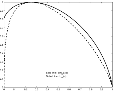
Figure 1. Spectra $\alpha\mapsto\dim_{H}E(\alpha)$ and $\alpha\mapsto F_{\rm inv}(\alpha)$ for $\varphi_{1}$.

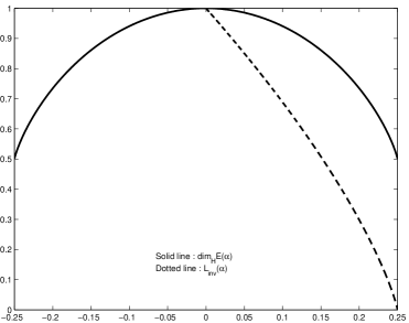
Figure 2. Spectra $\alpha\mapsto\dim_{H}E(\alpha)$ and $\alpha\mapsto F_{\rm inv}(\alpha)$ for $\varphi_{2}$.

5.2. Telescopic product measures

One of the key points in the proof of the Hausdorff spectrum (Theorem 17) is the observation that the coordinates $x_{1},\cdots,x_{n},\cdots$ of $x$ appearing in the definition of ${A}_{n}\varphi(x)$ share the following independence. Consider the partition of $\mathbb{N}^{*}$:

$$\mathbb{N}^{*}=\bigsqcup_{i\geq 1,q\nmid i}\Lambda_{i}\ \ {\rm with}\ \Lambda_{i}=\{iq^{j}\}_{j\geq 0}.$$

Observe that if $k=iq^{j}$ with $q\nmid i$, then $\varphi(x_{k},x_{kq},\cdots,x_{kq^{d-1}})$ depends only on $x_{|_{\Lambda_{i}}}$, the restriction of $x$ on $\Lambda_{i}$. So the summands in the definition of ${A}_{n}\varphi(x)$ can be put into different groups, each of which depends on one restriction $x_{|_{\Lambda_{i}}}$. For this reason, we decompose $\Sigma_{m}$ as follows:

$$\Sigma_{m}=\prod_{i\geq 1,q\nmid i}\mathcal{A}^{\Lambda_{i}}.$$

Telescopic product measures are now constructed as follows. Let $\mu$ be a probability measure on $\Sigma_{m}$. Notice that $\mathcal{A}^{\Lambda_{i}}$ is nothing but a copy of $\Sigma_{m}$. We consider $\mu$ as a measure on $\mathcal{A}^{\Lambda_{i}}$ for every $i$ with $q\nmid i$. Then we define the infinite product measure $\mathbb{P}_{\mu}$ on $\prod_{i\geq 1,q\nmid i}\mathcal{A}^{\Lambda_{i}}$ of the copies of $\mu$. More precisely, for any word $u$ of length $n$ we define

$$\mathbb{P}_{\mu}([u])=\prod_{i\leq n,q\nmid i}\mu([u_{|_{\Lambda_{i}}}]),$$

where $[u]$ denotes the cylinder of all sequences starting with $u$. The probability measure $\mathbb{P}_{\mu}$ is called telescopic product measure. Kenyon, Peres and Solomyak [51] have first constructed these measures.

The Hausdorff dimension of every telescopic product measure is computable.

Theorem 18.

([51, 30]) For any given measure $\mu$, the telescopic product measure $\mathbb{P}_{\mu}$ is exact and its dimension is equal to

$$\dim_{H}\mathbb{P}_{\mu}=\dim_{P}\mathbb{P}_{\mu}=\frac{(q-1)^{2}}{\log m}\sum_{k=1}^{\infty}\frac{H_{k}(\mu)}{q^{k+1}}$$

where $H_{k}(\mu)=-\sum_{a_{1},\cdots,a_{k}\in S}\mu([a_{1}\cdots a_{k}])\log\mu([a_{1}\cdots a_{k}]).$

5.3. Dimension formula of Ruelle-type

The function $\psi_{s}$ defined by (5.3) and (5.4) determine a special telescopic product measure which plays the role of Gibbs measure in the proof of the Hausdorff spectrum.

First we define a $(d-1)$-step Markov measure on $\Sigma_{m}$, which will be denoted by $\mu_{s}$, with the initial law

$$\pi_{s}([a_{1},\cdots,a_{d-1}])=\prod_{j=1}^{d-1}\frac{\psi_{s}(a_{1},\cdots,a_{j})}{\psi_{s}^{q}(a_{1},\cdots,a_{j-1})}$$ (5.6)

and the transition probability

$$Q_{s}\left([a_{1},\cdots,a_{d-1}],[a_{2},\cdots,a_{d}]\right)=e^{s\varphi(a_{1},\cdots,a_{d})}\frac{\psi_{s}(a_{2},\cdots,a_{d})}{\psi_{s}^{q}(a_{1},\cdots,a_{d-1})}.$$ (5.7)

The corresponding telescopic product measure $\mathbb{P}_{\mu_{s}}$ is proved to be a dimension maximizing measure of $E(\alpha)$ if $s$ is chosen to be the solution of $P^{\prime}_{\varphi}(s)=\alpha.$ The dimension of $\mathbb{P}_{\mu_{s}}$ is simply expressed by the pressure function. In other words, we have the following formula of Ruelle-type.

Theorem 19.

([30]) For any $s\in\mathbb{R}$, we have

$$\dim_{H}\mathbb{P}_{\mu_{s}}=\frac{1}{q^{d-1}}[P_{\varphi}(s)-sP^{\prime}_{\varphi}(s)].$$

5.4. Multiplicatively invariant sets

Kenyon, Peres and Solomyak [51] were able to compute both the Hausdorff dimension and the box dimension of $X_{2}$, already considered in §2.2, and of a class of generalizations of $X_{2}$. Peres, Schmeling, Seuret and Solomyak [61] generalized the results to a more general class of sets.

Recall that $\Sigma_{m}=\{0,1,...,m-1\}^{\mathbb{N}^{*}}$, $q$ is an integer greater than 2 and $\Lambda_{i}:=\{i\,q^{n}:n\geq 0\}$. For any subset $\Omega\subset\Sigma_{m}$, define

$$X_{\Omega}:=\{x=(x_{k})_{k\geq 1}\in\Sigma_{m}:\forall\,i\neq 0\!\!\!\mod q,\ x_{|\Lambda_{i}}\in\Omega\}.$$ (5.8)

We get $X_{\Omega}=X_{2}$ when $q=2$ and $\Omega$ is the Fibonacci set $\{y\in\Sigma_{m}:\forall\,k\geq 1,\ y_{k}y_{k+1}=0\}$.

The set $X_{\Omega}$ is not shift-invariant but is multiplicatively invariant in the sense that $M_{r}X_{\Omega}\subset X_{\Omega}$ for every integer $r\in\mathbb{N}^{*}$ where $M_{r}$ maps $(x_{n})$ to $(x_{rn})$.

The generating set $\Omega$ has a tree of prefixes, which is a directed graph $\Gamma$. The set $V(\Gamma)$ of vertices consists of all possible prefixes of finite length in $\Omega$, i.e.

$$V(\Gamma):=\bigcup_{k\geq 0}\mbox{Pref}_{k}(\Omega),$$

where $\mbox{Pref}_{0}(\Omega)=\{\emptyset\}$, $\mbox{Pref}_{k}(\Omega):=\{u\in\{0,1,...,m-1\}^{k}:\Omega\cap[u]\neq\emptyset\}$. There is a directed edge from a vertex $u$ to another $v$ if and only if $v=ui$ for some $i\in\{0,1,...,m-1\}$.

Theorem 20.

([51]) There exists a unique vector $\bar{t}=(t_{v})_{v\in\Gamma}\in[1,m^{\frac{1}{q-1}}]^{V(\Gamma)}$ defined on the tree such that

$$\forall v\in V(\Gamma),\ \ \ (t_{v})^{q}=\sum_{i\in\{0,1,...,m-1\}:\ vi\in\Omega}\ t_{vi}.$$ (5.9)

The Hausdorff dimension and the box dimension of $X_{\Omega}$ are respectively equal to

$$\dim_{H}(X_{\Omega}) = (q-1)\log_{m}t_{\emptyset}$$ (5.10)

$$\dim_{B}(X_{\Omega}) = (q-1)^{2}\sum_{k=1}^{+\infty}\frac{\log_{m}\left|\text{{\em Pref}}_{k}(\Omega)\right|}{q^{k+1}}.$$ (5.11)

The two dimensions coincide if and only if the tree $\Gamma$ is spherically symmetric, i.e. all prefixes of length $k$ in $\Omega$ have the same number of continuations of length $k+1$ in $\Omega$.

The vector $\bar{t}$ defines a measure $\mu$ on $\Omega\subset\{0,1,\cdots,m-1\}^{\mathbb{N}^{*}}$. Then a telescopic product measure can be built on $X_{\Omega}$. It is proved in [51] that there is a maximizing measure on $X_{\Omega}$ of this form.

A typical example of the class of sets studied by Peres, Schmeling, Solomyak and Seuret [61] is

$$X_{2,3}=\{x\in\Sigma_{m}:x_{k}x_{2k}x_{3k}=0\}.$$

The construction of the sets is as follows. Let $\kappa\geq 1$ be an integer and let $p_{1},\ldots,p_{\kappa}$ be $\kappa$ primes, which generates a semigroup $S$ of $\mathbb{N}^{*}$:

$$S=\langle p_{1},p_{2},\cdots,p_{\kappa}\rangle=\{p_{1}^{\alpha_{1}}p_{2}^{\alpha_{2}}\cdots p_{\kappa}^{\alpha_{\kappa}}:\alpha_{1},...,\alpha_{\kappa}\in\mathbb{N}\}.$$

The elements of $S$ are arranged in increasing order and denoted by $\ell_{k}$ the $k$-th element of $S=\{\ell_{k}\}_{k=1}^{\infty}:1=\ell_{1}<\ell_{2}<\cdots.$ Define

$$\gamma(S):=\sum_{k=1}^{\infty}\frac{1}{\ell_{k}}\,.$$ (5.12)

Write $(i,S)=1$ when $(i,p_{j})=1$ for all$j\leq\kappa$. We have the following partition of $\mathbb{N}^{*}$:

$$\mathbb{N}^{*}=\bigsqcup_{(i,S)=1}iS.$$ (5.13)

For each element $x={(x_{k})}_{k=1}^{\infty}$, $x|_{iS}$ denotes the restriction $x|_{iS}:={(x_{i\ell_{k}})}_{k=1}^{\infty}$, which is also viewed as an element of $\Sigma_{m}$. Given a closed subset $\Omega\subset\Sigma_{m}$, we define a new subset of $\Sigma_{m}$:

$$X_{\Omega}^{(S)}:=\Bigl{\{}x={(x_{k})}_{k=1}^{\infty}\in\Sigma_{m}:\ x|_{iS}\in\Omega\ \ \mbox{for all}\ i,\ (i,S)=1\Bigr{\}}.$$ (5.14)

Theorem 21.

([61]) There exists a vector $\overline{t}=(t(u))_{u\in{\rm Pref}(\Omega)}\in[1,+\infty)^{{\rm Pref}(\Omega)}$ defined on the tree of prefixes of $\Omega$ such that

$$t(\varnothing)\in[1,m],\ \ t(u)\in[1,m^{\ell_{k}(\ell_{k+1}^{-1}+\ell_{k+2}^{-1}+\cdots)}],\ |u|=k,\ k\geq 1,$$

which is the solution of the system

$$t(\varnothing)^{\gamma(S)} = \sum_{j=0}^{m-1}t(j),$$

$$t(u)^{\ell_{k+1}/\ell_{k}} = \sum_{j:\ uj\in{\rm Pref}_{k+1}(\Omega)}t(uj),\ \ \ \forall\ u\in{\rm Pref}_{k}(\Omega),\ \forall k\geq 1.$$

The Hausdorff dimension and the box dimension of $X_{\Omega}^{(S)}$ are respectively equal to

$$\dim_{H}(X_{\Omega}^{(S)}) = \log_{m}t(\varnothing)$$

$$\dim_{B}(X_{\Omega}^{(S)}) = \gamma(S)^{-1}\sum_{k=1}^{\infty}\Bigl{(}\frac{1}{\ell_{k}}-\frac{1}{\ell_{k+1}}\Bigr{)}\log_{m}|{\rm Pref}_{k}(\Omega)|.$$

We have $\dim_{H}(X_{\Omega}^{(S)})=\dim_{B}(X_{\Omega}^{(S)})$ if and only if the tree of prefixes of $\Omega$ is spherically symmetric.

Ban, Hu and Lin [2] studied the Minkowski dimension of $X_{2,3}$ and of some other multiplicative sets as pattern generating problem.

6. Remarks and Problems

6.1. Vector valued potential

The non-linear thermodynamic formalism can be generalized to vectorial potentials. Let $\varphi,\gamma$ be two functions defined on $\mathcal{A}^{\ell}$ taking real values. Instead of considering the transfer operator $\mathcal{L}_{s}$ as defined in (5.2), we consider the following one:

$$\mathcal{L}_{s}\psi(a)=\sum_{j\in S}e^{s\varphi(a,j)+\gamma(a,j)}\psi(Ta,j),\ a\in S^{\ell-1},\ s\in\mathbb{R}.$$

There exists a unique solution to the equation

$$(\mathcal{L}_{s}\psi)^{\frac{1}{q}}=\psi.$$

Then we define the pressure function $P_{\varphi,\gamma}(s)$ as indicated in $P_{\varphi,\gamma}(s)$. The function $s\mapsto P_{\varphi,\gamma}(s)$ is convex and analytic. Now, let $\underline{\varphi}=(\varphi_{1},\cdots,\varphi_{d})$ be a function defined on $S^{\ell}$ taking values in $\mathbb{R}^{d}$. For $\underline{s}=(s_{1},\cdots,s_{d})\in\mathbb{R}^{d}$, we consider the following transfer operator.

$$\mathcal{L}_{\underline{s}}\psi(a)=\sum_{j\in S}e^{\langle\underline{s},\underline{\varphi}\rangle}\psi(Ta,j),\ a\in S^{\ell-1},$$

where $\langle\cdot,\cdot\rangle$ denotes the scalar product in $\mathbb{R}^{d}$. We denote the associated pressure function by $P(\underline{\varphi})(\underline{s})$. Then for any vectors $u,v\in\mathbb{R}^{d}$ the function

$$\mathbb{R}\ni s\ \longmapsto\ P(\underline{\varphi})(us+v)$$

is analytic and convex. We deduce from this that the function $\underline{s}\ \mapsto\ P(\underline{\varphi})(\underline{s})$ is infinitely differentiable and convex on $\mathbb{R}^{d}$.

Similarly, we define the level sets $E(\underline{\alpha})$ $(\underline{\alpha}\in\mathbb{R}^{d})$ of $\underline{\varphi}$. A vector version of Theorem 17 is stated by just replacing the derivative of the pressure function by the gradient.

6.2. Invariant spectrum and mixing spectrum

The set $E_{\Phi}(\alpha)$ defined by (1.4) is not invariant. The size of the invariant part of $E_{\Phi}(\alpha)$ could be considered to be

$$d_{\rm inv}(\alpha)=\sup\{\dim^{*}\mu:\mu\ {\rm invariant},\ \mu(E_{\Phi}(\alpha))=1\}.$$

The function $\alpha\mapsto d_{\rm inv}(\alpha)$ is called the invariant spectrum of $\Phi$. Similarly we define the mixing spectrum of $\Phi$ by

$$d_{\rm mix}(\alpha)=\sup\{\dim^{*}\mu:\mu\ {\rm mixing},\ \mu(E_{\Phi}(\alpha))=1\}.$$

Examples in [30] show that it is possible to have

$$d_{\rm mix}(\alpha)<d_{\rm inv}(\alpha)<d_{H}(\alpha).$$

6.3. Semigroups

The semigroup $\{q^{n}\}_{n\geq 0}$ of $\mathbb{N}^{*}$ appeared in [30, 51]. Other semigroup structures appeared in [61]. Combining the ideas in [61, 30], averages like

$$\lim_{n\to\infty}\frac{1}{n}\sum_{k=1}^{n}\varphi(x_{k},x_{2k},x_{3k})$$

can be treated [73]. The Riesz product method used in [27] is well adapted to the study of the special limit on $\Sigma_{2}$:

$$\lim_{n\to\infty}\frac{1}{n}\sum_{k=1}^{n}(2x_{k}-1)(2x_{2k}-1)\cdots(2x_{\ell k}-1)$$

where $\ell\geq 2$ is any integer.

6.4. Subshifts of finite type

What we have presented is strictly restricted to the full shift dynamics. It is a challenging problem to study the dynamics of subshift of finite type and the dynamics with Markov property. New ideas are needed to deal with these dynamics. It is also a challenging problem to deal with potential depending more than one coordinates.

The doubling dynamics $Tx=2x$ $\!\!\!\!\mod 1$ on the interval $[0,1)$ is essentially a shift dynamics. Cookie cutters are the first interval maps coming into the mind after the doubling map. If the cookie cutter maps are not linear, it is a difficult problem. A cookie-cutter can be coded, but the non-linearity means that the derivative is a potential depending more than one codes.

Based on the computation made in [63], Liao and Rams [54] considered a special piecewise linear map of two branches defined on two intervals $I_{0}$ and $I_{1}$ and studied the following limit

$$\lim_{n\to\infty}\frac{1}{n}\sum_{k=1}^{n}1_{I_{1}}(T^{k}x)1_{I_{1}}(T^{2k}x).$$

The techniques presented in [30] can be used to treat the problem for general piecewise linear cookie cutter dynamics [28, 73].

6.5. Discontinuity of spectrum for V-statistics

The limit of V-statistics

$$\lim_{n\to\infty}n^{-r}\sum_{1\leq i_{1},\cdots,i_{r}\leq n}\Phi(T^{i_{1}}x,\cdots,T^{i_{r}}x).$$

was studied in [31] where it is proved that the multifractal spectrum of topological entropy of the above limit is expressed by an variational principle when the system satisfies the specification property. Unlike the classical case ($r=1$) where the spectrum is an analytic function when $\Phi$ is Hölder continuous, the spectrum of the limit of higher order V-statistics ($r\geq 2$) may be discontinuous even for very regular kernel $\Phi$. It is an interesting problem to determine the number of discontinuities. M. Rauch [68] has recently established a variational principe relative to $V$-statistics.

6.6. Mutual absolute continuity of two Riesz products

Let us state two conjectures. See [15] for the discussion on these conjectures.

Conjecture 1. Let $\mu_{a}$ and $\mu_{b}$ be two Riesz products and let $\omega:=(\omega_{n})\in G^{\mathbb{N}}$. Then $\mu_{a}\ll\mu_{b}\Rightarrow\mu_{a,\omega}\ll\mu_{b,\omega}$, and $\mu_{a}\perp\mu_{b}\Rightarrow\mu_{a,\omega}\perp\mu_{b,\omega}$.

For a function $f$ defined on $G$, we use $\mathbb{E}f$ to denote the integral of $f$ with respect to the Haar measure. The truthfulness is that the preceding conjecture implies the following one.

Conjecture 2. Let $\mu_{a}$ and $\mu_{b}$ be two Riesz products. Then

$$\prod_{n=1}^{\infty}\mathbb{E}\sqrt{(1+\mbox{\rm Re}\ a_{n}\gamma_{n})(1+\mbox{\rm Re}\ b_{n}\gamma_{n})}>0\Longrightarrow\mu_{a}\ll\mu_{b};$$

$$\prod_{n=1}^{\infty}\mathbb{E}\sqrt{(1+\mbox{\rm Re}\ a_{n}\gamma_{n})(1+\mbox{\rm Re}\ b_{n}\gamma_{n})}=0\Longrightarrow\mu_{a}\perp\mu_{b}.$$

6.7. Doubling and tripling

For any integer $m\geq 2$, we define the dynamics $\tau_{m}x=mx$ ($\!\!\!\!\mod 1$) on $[0,1)$. A typical couple of commuting transformations is the couple $(\tau_{2},\tau_{3})$. Let us take, for example, $\Phi(x,y)=e^{2\pi i(ax+by)}$ with $a,b$ being two fixed integers. We are then led to the multiple ergodic averages, a special case of (1.3),

$$A_{n}^{(2,3)}(x):=\frac{1}{n}\sum_{k=1}^{n}e^{2\pi i(a2^{k}+b3^{k})x}.$$ (6.1)

This is an object not yet well studied in the literature (but if $a=0$, we get a classical Birkhoff average). We propose to develop a thermodynamic formalism by studying Gibbs type measures which are weak limits $\mu_{s,t}$ ($s,t\in\mathbb{R}$) of

$$Z_{n}(s,t)^{-1}Q_{n}(x)dx$$

where

$$Q_{n}(x):=\prod_{k=1}^{n}e^{s\cos(2\pi(a2^{k}+b3^{k})x)+t\sin(2\pi(a2^{k}+b3^{k})x)}.$$

The pressure function defined by

$$P(s,t):=\lim_{n\to\infty}\frac{\log Z_{n}(s,t)}{n}$$

would be differentiable. But first we have to prove the existence of the limit defining $P(s,t)$.

More generally, let $(c_{n})$ be a sequence of complex numbers and $(\lambda_{n})$ a lacunary sequence of positive integers (by lacunary we mean $\inf_{n}\frac{\lambda_{n+1}}{\lambda_{n}}>1$). We can consider the following weighted lacunary trigonometric averages

$$\frac{1}{n}\sum_{k=1}^{n}c_{k}e^{2\pi i\lambda_{k}x}.$$

Under the divisibility condition $\lambda_{n}|\lambda_{n+1}$, such averages and more general averages were studied in [21]. For example, if $c_{k}=e^{2\pi i\omega_{k}}$ with $(\omega_{k})$ being an i.i.d. sequence of Lebesgue distributed random variables, from the results obtained in [21] we deduce that almost surely the pressure is well defined and equal to the following deterministic function

$$P(s,t)=\log\int_{0}^{2\pi}e^{\sqrt{t^{2}+s^{2}}\cos x}\frac{dx}{2\pi}.$$

Recall that

$$J_{0}(r)=\frac{1}{2\pi}\int_{0}^{2\pi}e^{r\cos x}dx=\sum_{n=0}^{\infty}\frac{r^{2n}}{(n!)^{2}2^{2n}}.$$

is the Bessel function.

But, the condition $\lambda_{n}|\lambda_{n+1}$ for $\lambda_{n}=2^{n}+3^{n}$ is not satisfied. Neither the condition is satisfied for $\lambda_{n}=2^{n}+4^{n}$. No rigorous results are known for the multifractal analysis of the averages defined by (6.1).

As conjectured by Fürstenberg, the Lebesgue measure is the unique continuous probability measure which is both $\tau_{2}$-invariant and $\tau_{3}$-invariant. However, common $\tau_{2}$- and $\tau_{3}$-periodic points (different from the trivial one $0$) do exists. Given two integers $n\geq 1$ and $m\geq 1$. We can prove that there is a point $x(\not=0)$ which is $n$-periodic with respect to $\tau_{2}$ and $m$-periodic with respect to $\tau_{3}$ if and only if

$$(2^{n}-1,3^{m}-1)>1.$$ (6.2)

Let $d=(2^{n}-1,3^{m}-1)$. When the above condition on GCD is satisfied, there are $d-1$ such common periodic points. These common periodic points $x(\not=0)$ are of the form $x=\frac{k}{2^{n}-1}=\frac{j}{3^{m}-1}$ for some $1\leq k<2^{n}-2$ and $1\leq j<3^{m}-2$. Actually choices for $k$ are

$$1\cdot\frac{2^{n}-1}{d},\ \ \ 2\cdot\frac{2^{n}-1}{d},\ \cdots,\ (d-1)\cdot\frac{2^{n}-1}{d}.$$

Choices for $j$ are $1\cdot\frac{3^{m}-1}{d},\ \ \ 2\cdot\frac{3^{m}-1}{d},\ \cdots,\ (d-1)\cdot\frac{3^{m}-1}{d}.$ Thus the $d-1$ common periodic points are $\frac{1}{d},\frac{2}{d},\cdots,\frac{d-1}{d}$. For such a point $x$, the following limit exists

$$\lim_{N\to\infty}A_{N}^{(2,3)}(x)=A_{nm}^{(2,3)}(x).$$

Note that there is an infinite number of such couples $n$ and $m$ such that (6.2) holds. There would be some relation between these common periodic points and the multifractal behavior of $A_{N}^{(2,3)}(x)$.

Bibliography

• [1]
• [2]   J. C. Ban, W. G. Hu and S. S. Lin, Pattern generating problems arising in multiplicative interger systems, preprint.
• [3] J. Barral and S. Seuret, Heterogeneous ubiquitous systems in $\mathbb{R}^{d}$ and Hausdorff dimension, Bull. Braz. Math. Soc. 38 no. 3 (2007), p. 467–515.
• [4] L. Barreira, Y. Pesin and J. Schmeling, Dimension and product structure of hyperbolic measures, Annals of Mathematics, 2nd ser. 149 (3) (1999), 755–783.
• [5] L. Barreira, B. Saussol and J. Schmeling, Higher dimensional multifractal analysis, J. Math. Pure. Appl. 81 (2002), p. 67–91.
• [6] V. Beresnevich and S. Velani, A mass transference principle and the Duffin-Schaeffer conjecture for Hausdorff measures, Ann. Math. 164 (2006), p. 971–992.
• [7] J. Bourgain, Double recurrence and almost sure convergence. J. Reine. Angew. Math. 404 (1990), 140-161.
• [8] R. Bowen, Topological entropy for noncompact sets, Trans. Amer. Math. Soc. 184 (1973), p. 125–136.
• [9]  G. Brown, G. Michon and J. Peyrière, On the multifractal analysis of measures, J. Statist. Phys. 66 (1992), p. 775–790.
• [10] P. Collet, J.L. Lebowitz, A. Porzio, The dimension spectrum of some dynamical systems, J. Stat. Phys. 47 (1987), p. 609–644.
• [11] Conze, J.P., Lesigne, E. Théorèmes ergodiques pour des mesures diag- onales, Bull. Soc. Math. France, 112 no. 2 (1984), 143-175.
• [12] C. Cutler, Connecting ergodicity and dimension in dynamical systems, Ergodic Theory Dynam. Systems 118 (1995), p. 393–410.
• [13] A. Durand, Ubiquitous systems and metric number theory, Adv. Math., 218 (2008), p. 368–394.
• [14] K. J. Falconer, Fractal Geometry: Mathematical Foundations and Applications, 2nd Edition. Wiley, 2003.
• [15] J. Barral, A. H. Fan and J. Peyrière, Quelques interactions entre analyse, probabilités et fractales, pp 57–189, in Panorama et Synthèse/SMF, No. 32 , 2010.
• [16] A.H. Fan, Recouvrement aléatoire et décompositions de mesures, Publication d’Orsay, 1989.
• [17] A.H. Fan, Quelques propriétés de produits de Riesz, Bull. Sci. Math. 117 (1993) no. 3, p. 421–439.
• [18] A.H. Fan, Sur les dimensions de mesures, Studia Math. 111 (1994) no.1, p. 1–17.
• [19] A.H. Fan, On ergodicity and unidimensionality, Kyushu J. Math. 48 (1994) no.2, p. 249–255.
• [20] A.H. Fan, Une formule approximative de dimension pour certains produits de Riesz, Monatshefte für Mathematik. 118 (1994) p. 83–89.
• [21] A.H. Fan, Multifractal analysis of infinite products, J. Stat. Phys. 86 (1997) nos.5/6, p. 1313–1336.
• [22] A.H. Fan Individual behaviors of oriented walks, Stoc. Proc. Appl., Stoc. Proc. Appl., 90 (2000) p. 263–275.
• [23] A.H. Fan and D. J.  Feng, On the distribution of long-term time averages on symbolic space, J. Statist. Phys. 99 (1999), p. 813–856.
• [24] A.H. Fan, D. J.  Feng and J. Wu, Recurrence, dimension and entropy, J. London. Math. Soc. 64 (2001), p. 229–244.
• [25] A.H. Fan, K. S. Lau and H. Rao, Relationship between different dimension of a measure, Monatsch. Math., 135 (2002), p. 191–201.
• [26] A.H. Fan, L.M. Liao and J. Peyrière, Generic points in systems of specification and Banach valued Birkhoff ergodic average, Discrete and continuous dynamical systems 21 (2008) no. 4, p. 1103–1128.
• [27] A.-H. Fan, L. Liao, J.-H. Ma, Level sets of multiple ergodic averages, Monatshefte für Mathematik, Volume 168, Issue 1 (2012); p 17–26.
• [28] A. H. Fan, L. M. Liao and M. Wu, Multifractal analysis of some multiple ergodic averages in linear Cookie-Cutter dynamical systems, preprint.
• [29] A.H. Fan and J. Schmeling, On fast Birkhoff averaging, Math. Proc. Camb. Phil. Soc. 135 (2003), p. 443–467.
• [30] A.-H. Fan, J. Schmeling and M. Wu, Multifractal analysis of some multiple ergodic average, preprint.
• [31] A.-H. Fan, J. Schmeling and M. Wu, Multifractal analysis of V-statistics, in Further Developments in Fractals and Related Fields, J. Barral and S. Seuret Ed. Trends in Mathematics, 2013, pp 135–151.
• [32] A.H. Fan, J. Schmeling and S. Troubetzkoy, A multifractal mass transference principle for Gibbs measures with applications to dynamical Diophantine approximation, to apper in Proc. London Math. Soc., (3) 107 (2013) 1173-1219.
• [33] A.H. Fan and M. Wu, Oriented walks on Euclidean spaces, preprint.
• [34] W. Feller, An introduction to probability Theory and Its Applications. Third Edition, vol. 1, John Wiley & Sons, 1968.
• [35] D.J. Feng, K.-S. Lau and J. Wu, Ergodic limits on the conformal repellers, Adv. Math. 169 (2002), p. 58–91.
• [36] U. Frisch and G. Parisi, Fully developped turbulence and intermittency in turbulence, and predictability in geophysical fluid dynamics and climate dymnamics, International school of physics ”Enrico Fermi”, course 88, edited by M. Ghil, North Holland (1985), p. 84.
• [37] H. Fürstenberg, Ergodic behavior of diagonal measures and a theorem of Szemerédi on arithmetic progressions. J. Anal. Math. 31 (1977), 204-256
• [38] H. Fürstenberg and B. Weiss, A mean ergodic theorem for $(1/N)\sum_{n=1}^{N}f(T^{n}x)g(T^{n^{2}}x)$. Convergence in ergodic theory and probability Ohio State Univ. Math. Res. Inst. Publ., 5, de Gruyter, Berlin, 193-227 (1996).
• [39] , H. Haase, A survey on the dimension of measures, Topology, Measures and Fractals (Warnemünde, 1991), Math. Res., vol. 66, Akademie Verlag, Berlin, 1992, pp. 66–75.
• [40] T.C. Halsey, M.H. Jensen, L.P. Kadanoff, I. Procaccia and B.I. Shraiman, Fractal measures and their singularities : the characterisation of strange sets, Phys. Rev. A   33 (1986), p. 1141.
• [41] H.G.  Hentschel and I. Procaccia, The infinite number of generalized dimensions of fractals and strange attractors, Physica 8D (1983), p. 435.
• [42] Y. Heurteaux, Estimations de la dimension inférieure et de la dimension supérieure des mesures, Ann. Inst. H. Poincaré Probab. Statist. 34 (1998), p. 309–338.
• [43] E. Hewitt and H.S. Zuckerman, Singular measures with absolutely continuous convolution squares, Proc. Camb. Phil. Soc. 62 (1966), p. 399–420.
• [44] B. Host, B. Kra, Nonconventional ergodci averages and nilmanifolds. Ann. Math. 161 (2005), 397-488.
• [45] J.D. Howroyd, On the theory of Hausdorff measures in metric spaces, Thesis, University fo London, 1994.
• [46] S. Jaffard, Multifractal formalism for functions. I. Results valid for all functions. II. Self-similar functions, SIAM J. Math. Anal. 28 (1997), p. 944–970 and p. 971–998.
• [47] J.-P. Kahane, Intervalles aléatoires et décomposition des mesures , C. R. Acad. Sci. Paris Sér.I. 304 (1987), 551–554.
• [48] J.-P. Kahane and J. Peyrière, Sur certaines martingales de Mandelbrot, Advances in Math. 22 (1976), p. 131–145.
• [49] S. Kakutani, On equivalence of infinite product measures, Ann. Math. 49 (1948), p. 214–224.
• [50] R. Kaufman, A ”min-max” theorem on potentials, C. R. Acad. Sci. Paris Sér. I Math. 319 (1994) no.8, p. 799–800.
• [51] R. Kenyon, Y. Peres, B. Solomyak, Hausdorff dimension for fractals invariant under the multiplicative integers, Erg. Th. Dyn. Syst., 32 no. 5 (2012), 1567–1584.
• [52] Y. Kifer, A nonconventional strong law of large numbers and fractal dimensions of some multiple recurrence sets, Stochastics and Dynamics, Vol. 12, No. 3 (2012).
• [53] E. Lesigne, Theorems ergodiques pour une translation sur une nilvariete, Erg. Thm and Dyn.Sys, 9 (1) (1989), 115-126.
• [54] L. M. Liao and M. Rams, Multifractal analysis of some multiple ergodic averages for the systems with non-constant Lyapunov exponents, Real Analysis Exchange, 39, no. 1(2013), 1-14.
• [55] B. Mandelbrot, Possible refinement of the log-normal hypothesis concerning the distribution of energy dissipation in intermittent trubulence in statistical models and trubulence, Symposium at U. C. San Diego 1971, Lecture Notes in Physics, Springer-Verlag 1972, p. 333–351.
• [56] B. Mandelbrot, Multiplications aléatoires itérées et distributions invariantes par moyennes pondérée aléatoire, C. R. Acad. Sci. Paris 278 (1974), p. 289–292.
• [57] B. Mandelbrot, Multiplications aléatoires itérées et distributions invariantes par moyennes pondérée aléatoire: quelques extensions, C. R. Acad. Sci. Paris 278 (1974), p. 355–358.
• [58] P. Mattila, Geometry of sets and measures in Euclidean spaces. Fractals and rectifiability, Cambridge Studies in Advanced Mathematics 44, Cambridge University Press, Cambridge, 1995.
• [59] E. Olivier, Multifractal analysis in symbolic dynamics and distribution of pointwise dimension for $g$-measures, Nonlinearity 12 (1999), p. 1571–1585.
• [60] L. Olsen, A multifractal formalism, Adv. Math.  116 (1995), p. 92–195.
• [61] Y. Peres, J. Schmeling, S. Seuret, B. Solomyak, Hausdorff dimension for fractals generated by multiplication by $2$ and $3$, Israel Journal of Math., to appear.
• [62] Y. Peres, B. Solomyak, Dimension spectrum for a nonconventional erdofic average, Real Analysis and Exchange, Vol. 37 (2), 2011/2012, pp. 375–388.
• [63] Y. Peres, B. Solomyak, The multiplicative golden mean shift has infinite Hausdorff measure, in Further Developments in Fractals and Related Fields, J. Barral and S. Seuret Ed. Trends in Mathematics, 2013, pp 193–212.
• [64] Y. Pesin, Dimension theory in dynamical systems: Contemporary views and applications, Chicago lectures in Mathematics, The University of Chicago Press, 1997.
• [65] J. Peyrière, Étude de quelques propriétés des produits de Riesz, Ann. Inst. Fourier 25 (1975), p. 127–169.
• [66] J. Peyrière, Almost everywhere convergence of lacunary trigonometric series with respect to Riesz products, Australian J. Math. (Series A) 48 (1990), p. 376–383.
• [67] D.A. Rand, The singularity spectrum $f(\alpha)$ for cookie-cutters, Ergod. Th. & Dynam. Syst. 9 (1989), p. 527–541.
• [68] M. Rauch, A Multivariate Variational Principle, Diploma Thesis, University of Jena, 2013.
• [69] D. Ruelle, Thermodynamic Formalism, Encyclopedia of Mathematics and its Applications, 5, Addison-Weysley, 1978.
• [70] F. Takens and E. Verbitskiy, On the variational principle for the topological entropy of certain non-compact sets, Ergod. Th. Dynam. Syst. 23 (2003) no. 1, p. 317–348.
• [71] M. Tamashira, Dimensions in a separable metric space, Kyushu J. Math. 49 (1995) no. 1, p. 143–162.
• [72] P. Walters, An introduction to ergodic theory, GTM 79. New York, Springer-Verlag, 1982.
• [73] M. Wu, Multifractal Analysis of Some Nonconventional Ergodic Averages, Ph D Thesis, University of Picardie Jules Verne, June 2013.
• [74] L.S. Young, Dimension, entropy and Lyapounov exponents, Erg. Th. Dynam. Syst. 2 (1982), p. 109–124.
• [75] T. Ziegler, A non-conventional ergodic theorem for a nilsystem. Erg. Th. Dynam. Syst. 25 (4) (2005), 1357–1370.
• [76] A. Zygmund, Trigonometric series. Cambridge University Press (1968).