Mechanism of the Cassie-Wenzel transition via the atomistic and continuum string methods

Abstract

The string method is a general and flexible strategy to compute the most probable transition path for an activated process (rare event). We apply here the atomistic string method in the density field to the Cassie-Wenzel transition, a central problem in the field of superhydrophobicity. We discuss in detail the mechanism of wetting of a submerged hydrophobic cavity of nanometer size and its dependence on the geometry of the cavity. Furthermore, we discuss the algorithmic analogies between the string method and CREaM [Giacomello et al., Phys. Rev. Lett. 109, 226102 (2012)], a method inspired by the string that allows for a faster and simpler computation of the mechanism and of the free-energy profiles of the wetting process. This approach is general and can be employed in mesoscale and macroscopic calculations.

I Introduction

Wetting of chemically and topographically heterogeneous surfaces gives rise to a rich phenomenology and a corresponding wealth of theoretical challenges.Quéré (2008); Rauscher and Dietrich (2008) A remarkable example is that a careful combination of surface roughness and chemistry yields highly liquid-repellent and self-cleaning surfaces under given environmental conditions: this class of properties is often referred to as superhydrophobicity. Superhydrophobicity is related to the trapping of gaseous pockets (air and/or vapor) inside surface roughness.Lafuma and Quéré (2003) We will loosely refer to this scenario as the Cassie state. The superhydrophobic Cassie state also favors the emergence of liquid slippage under flow conditions.Tretyakov and Müller (2013); Gentili et al. (2014) However, superhydrophobicity breaks down as soon as the surface roughness becomes wet in the so-called Wenzel state. As a consequence of the very different properties of the Cassie and Wenzel states, there is a growing interest in designing surfaces that are capable of stabilizing the superhydrophobic Cassie state. In order for such engineering effort to be effective, a thorough knowledge of the Cassie-Wenzel transition is required. With this objective, we analyze here the mechanism of the Cassie-Wenzel transition with the string method applied to molecular dynamics simulations.

The phase transition between the Cassie and the Wenzel states is, in most cases, characterized by large free-energy barriers.Dupuis and Yeomans (2005); Koishi et al. (2009); Savoy and Escobedo (2012); Giacomello et al. (2012a); Checco et al. (2014) The superhydrophobic Cassie state on the same surface can be stable, metastable , or unstable depending on the environmental conditions. Therefore it is not correct to speak about superhydrophobic surfaces, but rather about superhydrophobic states.Lafuma and Quéré (2003) The problem of designing surfaces with superhydrophobic properties is therefore one of maximizing the range of temperatures, pressures, and characteristics of the liquids/vapor phases in contact for which the Cassie state is stable. In the conditions where the Cassie state is not thermodynamically stable, it is nonetheless possible to exploit metastabilities to obtain long-living superhydrophobicity: this is the case, e.g., of omniphobic surfaces that present a metastable Cassie state even with “wetting” liquids thanks to a special reentrant geometry.Tuteja et al. (2007) Indeed, free-energy barriers must be much larger than the thermal energy $k_{B}T$ in order for the metastable Cassie state to survive for times that are significant for experiments and applications. Knowledge of how the Cassie-Wenzel transition starts and evolves –the transition path or wetting mechanism– may yield new insights for the design of engineered surfaces.

According to the transition state theory, the rate of the Cassie-Wenzel transition depends exponentially on the free-energy barrier between these two states. Thus, designing surfaces with the desired Cassie-Wenzel free-energy barrier is an effective tool for controlling the rate of the process. For instance it has recently been suggestedPoetes et al. (2010) that the Cassie state is generally metastable underwater. This statement, which is based on experiments on a small number of surfaces, could be made more precise if the way in which free-energy barriers depend on the geometry of the surface roughness was known. The crucial point for applications is not whether the desired state is metastable or stable but whether it will last longer than the experiment/application. The first step in engineering surfaces is, therefore, the characterization of the wetting mechanism and of its dependence on the topography and chemistry of the surface, as well as on the thermodynamic conditions.

Previous works typically considered the mechanism of the Cassie-Wenzel transition on drops, see e.g. Ref. Kusumaatmaja et al., 2008; Papadopoulos et al., 2013, but there is a growing interest in submerged surfaces where the external pressure plays a key role in the stability of the superhydrophobic state. We focus here on the latter case by studying a model system that is simple enough to allow comparison of different approaches and yet shows a surprisingly rich phenomenology (see Fig. 1).

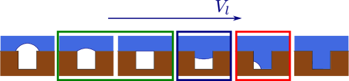
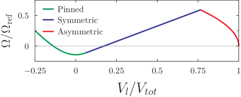
Figure 1: Mechanism of the Cassie-Wenzel transition on rectangular grooves as computed with the continuum rare events methodGiacomello et al. (2012a) (top): the path is parameterized in terms of the volume of liquid filling the cavity, $V_{l}$. Free-energy profile of the Cassie-Wenzel transition as computed from the path above at coexistence (bottom).

In previous works Giacomello et al. (2012b, a, 2013) we characterized the free-energy barriers of the Cassie-Wenzel transition occurring in isolated hydrophobic roughness elements under different conditions of pressure and temperature. The systems considered spanned from few nanometers (explored via molecular dynamics simulationsGiacomello et al. (2012b)) to macroscopic dimensions, for which the Continuum Rare Events Methods, or CREaM, was developed.Giacomello et al. (2012a, 2013) Over this broad range of systems, at coexistence –when the Cassie and Wenzel state have the same free-energy–, free-energy barriers are much larger than $k_{B}T$ accounting for strong metastabilities.

For all previous approaches, the wetting path was characterized following the changes in the (coarse-grained) density field of the fluid, $\rho(x)$. This, in turn, was considered a parametric function of the filling of the surface corrugation (or liquid volume inside it), $\rho(x;V_{l})$. The resulting path of the transition is the sequence $\{\rho(x;V_{l,i})\}_{i=1,N}$ of density fields minimizing the free-energy at a given $V_{l,i}$. Under suitable conditions, explained in Sec. IV, this represent a realistic description of the wetting path. However, when this description was applied in combination with a macroscopic, sharp-interface macroscopic model,Giacomello et al. (2012a) we obtained a discontinuous wetting path (see Fig. 1). The discontinuity corresponds to an instantaneous switching from a symmetric liquid/vapor meniscus to an asymmetric bubble in one of the corners of the corrugation (morphological transition). This discontinuity occurs at the “transition state” and results in a non-differentiability of the free energy profile at this point. This sharp point may have two distinct origins,

• an algorithmic one, related to the parameterization of the wetting path with the volume of liquid in the groove used in CREaM

• a modeling one, that is, it could arise as a genuine feature of the sharp-interface model, which was used in combination with CREaM.Giacomello et al. (2012a, 2013)

The goal of this paper is therefore to address the question about the sharp point of the free-energy profile and, more generally, to lay on solid statistical grounds the discussion about the wetting mechanism on rough surfaces. In order to achieve this goal, we compute the minimum free-energy path (MFEP) using the string method in collective variables.Maragliano et al. (2006) We employ atomistic simulations with the aim of making minimal assumptions on the liquid/vapor interface and the interactions with the walls. The collective variable that characterizes the microscopic configuration implemented is the coarse-grained density field. We compare atomistic with continuum, sharp-interface model paths and free-energy profiles. The continuum path is obtained with the string and CREaM methods. Qualitatively, the atomistic and continuum wetting are consistent. Surprisingly, atomistic string free-energy profile shows a better agreement with continuum CREaM. This is due to an “error cancellation”, with CREaM compensating intrinsic limitations in the sharp-interface model with respect to the atomistic case.

The second goal of this work is to elucidate the effect of the shape of the surface corrugation and its size on the mechanism of the Cassie-Wenzel transition and on the related free-energy barrier. Anticipating our results, the concept of transition path itself may break down if the corrugations are sufficiently small.

The paper is organized as follows: in Sections II, III, and IV the methods employed here, the atomistic string, the interface string, and the continuum rare events method (CREaM) are introduced and compared. This first part contains the main methodological findings. In Section V the atomistic and continuum results are presented and discussed, concentrating on the physics of the Cassie-Wenzel transition. The last section summarized all conclusions.

II Molecular Dynamics Simulations

The mechanism of the Cassie-Wenzel transition was investigated with the string method in collective variables applied to molecular dynamics simulationsMaragliano et al. (2006). Molecular dynamics simulations were performed with the LAMMPS enginePlimpton (1995) equipped for the string calculations with the PLUMEDBonomi et al. (2009) plugin as explained below. The isothermal/isobaric ensemble (NPT) was used for all simulations by using the algorithm of Martyna et al.Martyna, Klein, and Tuckerman (1992); Martyna, Tobias, and Klein (1994). The standard Lennard Jones (LJ) potential was used for the fluid-fluid interactions; fluid-solid interactions were also of LJ type, with the attractive term that was tuned through the factor $c$:

$$\Phi_{LJ}(r_{ij})=\epsilon\left[\left(\frac{\sigma}{r_{ij}}\right)^{12}-c\left(\frac{\sigma}{r_{ij}}\right)^{6}\right]\text{ ,}$$ (1)

where $r_{ij}$ is the distance between the atoms $i$ and $j$, while $\epsilon$ and $\sigma$ set the scales of energy and length, respectively. In order to obtain a hydrophobic solid, we set $c=0.6$, which corresponds to a contact angle of $\theta_{Y}\simeq 110^{\circ}$. Periodic boundary conditions are applied in the three directions. The lower wall featured a rectangular groove (or trench) extending through the $y$ direction. Two kinds of grooves were considered, the first having a width of $11\sigma$ and square aspect ratio and the second having a width of $22\sigma$ and a rectangular aspect ratio, see Fig. 2.

II.1 Coarse grained density field

The collective variable used to describe the intrusion of liquid inside of the groove was the coarse-grained density field. This quantity was computed from the atomic positions as the number of atoms inside the cells sketched in Fig. 2. We used a mollified version of the characteristic function of the cells based on the Fermi functions in order to prevent impulsive forces on atoms crossing the cell boundaries (see Sec. II.2). The cells occupied the whole $y$ dimension of the groove thus being effectively two-dimensional: for the square groove a total of $N=66$ cells were used, while for the rectangular groove $N=120$, as sketched in Fig. 2.

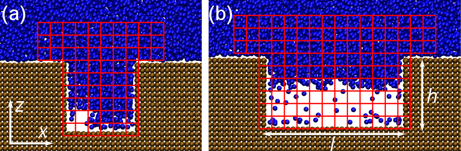
Figure 2: Cells used in the definition of the coarse-grained density collective variable for the square (a) and the rectangular groove (b). The axes and relevant dimensions used in the text are also defined.

The Landau free-energy of the system as a function of the realization, $\bm{z}$, of the (vector) collective variable $\bm{\theta}(\bm{r})$ is defined as:

$$F(\bm{z})=-k_{B}T\ln P(\bm{z})=-k_{B}T\ln\left(\int\mathrm{d}\bm{r}\;\;\mathrm{m}(\bm{r})\prod_{i=1}^{N}\delta(\theta_{i}(\bm{r})-z_{i})\;\right)\text{ ,}$$ (2)

where $k_{B}$ is the Boltzmann constant, $T$ is the system temperature, $P(\bm{z})$ is the probability to find the system at state $\bm{z}$, and $\bm{r}$ is the $3N_{p}$ dimensional vector of particles positions, with $N_{p}$ the number of particles in the system. The probability $P(\bm{z})$ is expressed in the second equality of Eq. (2) as the integral over the $3N_{p}$-dimensional configurational space of the probability density $\mathrm{m}(\bm{r})$ of the relevant ensemble (the Boltzmann factor) times Dirac deltas centered at value $z_{i}$ of the $N$ components of the collective variable. The collective variable is assumed to depend only on the $3N_{p}$ configurational degrees of freedom.

II.2 Implementation of the string method

For the general derivation of the string method in collective variables we refer the reader to the original work of Maragliano et al.Maragliano et al. (2006) Briefly, this method allows one to identify the minimum free-energy path (MFEP), that is, the path of maximum likelihood. The MFEP is the continuous curve in the space of collective variables –in this case the coarse-grained density field– satisfying the equation

$$\frac{dz_{i}(\alpha)}{d\alpha}\quad\bigg{\lvert}\bigg{\rvert}\quad\sum_{j=1}^{N}M_{ij}(\bm{z}(\alpha))\frac{\partial F(\bm{z}(\alpha))}{\partial z_{j}}\text{ ,}$$ (3)

where $\alpha$ is a parameterization of the MFEP, $\parallel$ means “parallel to”, the indices $i$ and $j$ run over the $N$ collective variables (which in vector notation are indicated as $\bm{z}$), $F(\bm{z})$ is the free-energy defined in Eq. (2), and $M_{ij}(\bm{z})$ is a metric matrix due to projection of the phase space onto the collective variable space, and defined asMaragliano et al. (2006)

$$M_{ij}(\bm{z}) = \langle{\bm{\nabla}}_{\bm{r}}\theta_{i}\cdot{\bm{\nabla}}_{\bm{r}}\theta_{j}\rangle_{\bm{z}}$$ (4)

$$\equiv \frac{\int\;\mathrm{d}\,\bm{r}\;\;{\bm{\nabla}}_{\bm{r}}\theta_{i}\cdot{\bm{\nabla}}_{\bm{r}}\theta_{j}\;\;\mathrm{e}^{-\beta U(\bm{r})}\prod_{k=1}^{N}\delta(\theta_{k}(\bm{r})-z_{k})}{\int\;\mathrm{d}\,\bm{r}\;\;\mathrm{e}^{-\beta U(\bm{r})}\prod_{k=1}^{N}\delta(\theta_{k}(\bm{r})-z_{k})}\text{ ,}$$

where $\beta^{-1}=k_{B}T$ and $U(\bm{r})$ is the potential energy of the system. Loosely speaking, when the metric matrix is unitary, Eq. (3) prescribes that the MFEP joins two minima of the free-energy landscape passing through the bottom of the valleys and the saddle point connecting them (the transition state).

The string method is an algorithm that allows one to identify the MFEP. The string itself is a discretization of the path connecting two metastable states, that is, two minima in the free-energy landscape. The string is parameterized according to its relative arc-length, $\alpha=\int_{{\bm{z}}_{a}}^{{\bm{z}}_{\alpha}}|\mathrm{d}\bm{z}|/\int_{{\bm{z}}_{a}}^{{\bm{z}}_{b}}|\mathrm{d}\bm{z}|$, with $a$ and $b$ beginning and end of the string. The discrete points along the string are called images and are labeled with their position on the string $\alpha_{l}$, where $l$ is the index of the images. We use here the version of the string method by E et al.E, Ren, and Vanden-Eijnden (2007), which consists of three steps:

1. Calculation of the free-energy gradient and of the metric matrix, see RHS of Eq. (3), at the current position of the images;

2. Evolution of one timestep of the images according to the (time-discretized) pseudo-dynamics

   $$\frac{\partial z_{i}(\alpha_{l},t)}{\partial t}=-\sum_{j=1}^{N}M_{ij}(\bm{z}(\alpha_{l},t))\frac{\partial F(\bm{z}(\alpha_{l},t))}{\partial z_{j}}\text{ ;}$$ (5)

3. Parameterization of the string to enforce equal arc-length parameterization among contiguous images.

For sufficiently large $t$, the algorithm guarantees that $z(\alpha_{l},t)$ converges to the MFEP of Eq. (3). Maragliano et al. (2006); E, Ren, and Vanden-Eijnden (2007)

Steps 2 and 3 of the string algorithm above can be written also asMaragliano et al. (2006)

$$\frac{d{\bm{z}}(\alpha_{l},t)}{dt}=-{\hat{M}}(\bm{z}(\alpha_{l},t))\nabla F(\bm{z}(\alpha_{l},t))\left(\bm{1}-\bm{\tau}(\bm{z}(\alpha_{l},t))\otimes\bm{\tau}(\bm{z}(\alpha_{l},t))\right)\,,$$ (6)

where the term $\bm{1}-\bm{\tau}(\bm{z}(\alpha_{l},t))\otimes\bm{\tau}(\bm{z}(\alpha_{l},t))$ projects out the component of $-{\hat{M}}(\bm{z}(\alpha_{l},t))\nabla F(\bm{z}(\alpha_{l},t))$ along the string. his projector, indeed, implements the constraint $\alpha=const.$ in the dynamics of $z(\alpha_{l},t)$ (see Eq. 2 of Ref. E, Ren, and Vanden-Eijnden (2007)). Summarizing, the string method is a first order dynamics with the constraint of constant value of the parameter $\alpha_{l}$ following the generalized force $-{\hat{M}}(\bm{z}(\alpha_{l},t))\nabla F(\bm{z}(\alpha_{l},t))$. In other words, the string method is a constrained (local) minimization of the system at a set of states at fixed $\alpha_{l}$ in a space equipped with the metric $\hat{M}$.

In order to compute the free-energy gradient and the metric matrix required to evolve the string via Eq. (5) (point $1.$ of the algorithm) we used restrained molecular dynamics (RMD, see Ref. Maragliano et al., 2006). In practice, a restraining potential was added to the Hamiltonian of the system in the form $\kappa/2(\theta_{i}(\bm{r})-z_{i})^{2}$, where $\theta_{i}(\bm{r})$ is the current value of the $i$-th component of the collective variable vector and $z_{i}$ is its target value. For sufficiently large $\kappa$, the dynamics driven by the restrained Hamiltonian samples the conditional ensemble at $\bm{\theta}(\bm{r})=\bm{z}$, and allows one to compute the relevant quantities at a given position of the string Maragliano et al. (2006).

II.3 Transition state ensemble

Once the string method has converged, it is possible to explore local approximations to the isocommittor surfaces, which are the hyperplanes orthogonal (via the metric $\hat{M}$) to the string. In particular, we considered here the hyperplane intersecting the string at the transition state; this plane bears the relevant information about the transition region, that is, the region where the probability to fall into the products’ side is the same as in the reactants’ Maragliano et al. (2006). The transition ensemble is a collection of microscopic states with the constraint that the system lies on this plane.

The transition state ensemble just discussed was computed via restrained molecular dynamics implementing the prescription

$$\sum_{i,j=1}^{N}\tau_{i}(\alpha_{TS})M_{ij}\left(\bm{z}(\alpha_{TS})\right)(z_{j}-z_{j}(\alpha_{TS}))=0\text{ ,}$$ (7)

where $\bm{\tau}(\alpha_{TS})$ is the tangent to the string at the transition state (TS). The configurations extracted from the transition state ensemble are discussed in Sec. V.

III The interface string

Rather than describing the configuration of the system by the coarse-grained density field, $\rho(x,z)$, one can characterize the configuration of the liquid inside the cavity by the position, $h_{i}$, of the liquid-vapor interface. Conceptually, one can obtain the corresponding Landau free-energy, $\Omega[h_{i}]$, by Eq. (2) using the collective variable, $h=\bm{\theta}(\bm{r})$. This strategy requires a definition of the interface position, $h$, in terms of the microscopic degrees of freedom, $\{{\bm{r}}\}$, which can be achieved via the coarse-grained density field.

In the following, however, we do not compute the Landau free-energy from the particle simulations but, instead, we use the mean-field, sharp-interface approximation to estimate $\Omega$. This grand potential takes the form Giacomello et al. (2012a)

$$\Omega=-p_{l}V_{l}-p_{v}V_{v}+\gamma_{lv}A_{lv}+\gamma_{sv}A_{sv}+\gamma_{sl}A_{sl}$$ (8)

where $V_{tot}$, $V_{l}$, and $V_{v}$ denote the total volume and the volumes occupied by the liquid and the vapor, respectively. $\gamma_{lv}$, $\gamma_{sl}$, and $\gamma_{sv}$ characterize the liquid-vapor interface tension, and the surface tension of the confining solid with the liquid and the vapor. $A_{lv}$, $A_{sl}$, and $A_{sv}$ are the contact areas of the three coexisting phases.

Additionally, like in capillary-wave Hamiltonians or solid-on-solid models, we assume that the interface position, $z=h_{i}(x)$, is a single-valued function, i.e., configurations with overhangs and bubbles are ignored. Using a completely filled cavity as reference state, $\Omega_{0}=-p_{l}V_{tot}+\gamma_{sl}l_{y}(2h+l)$ with $h$ being the height of the cavity and $l$ its widths, we obtain for the excess grand potential $\Delta\Omega=\Omega-\Omega_{0}$

$$\Delta\Omega = (p_{l}-p_{v})V_{v}+\gamma_{lv}A_{lv}+(\gamma_{sv}-\gamma_{sl})A_{sv}$$ (9)

$$\frac{\Delta\Omega}{V_{tot}\Delta p_{\max}} = \Delta\tilde{p}\frac{V_{v}}{V_{tot}}-\frac{lA_{lv}}{2V_{tot}\cos\theta_{Y}}-\frac{lA_{sv}}{2V_{tot}}$$ (10)

with the abbreviations $\Delta p_{\max}=-2\gamma_{lv}\cos\theta_{Y}/l$, $\Delta\tilde{p}=\frac{p_{l}-p_{v}}{\Delta p_{\max}}$, and Young’s equation $\gamma_{lv}\cos\theta_{Y}=\gamma_{sv}-\gamma_{sl}$.

Next, we express the vapor volume, $V_{v}$, the interface area, $A_{lv}$, and the solid-vapor contact area, $A_{sv}$, through the interface position, $h_{i}(x)$

$$\frac{V_{v}}{V_{tot}} = \frac{1}{lh}\int_{0}^{l}{\rm d}x\;h_{i}(x)$$ (11)

$$\frac{lA_{lv}}{V_{tot}} = \frac{1}{h}\int_{0}^{l}{\rm d}x\;\sqrt{1+\left(\frac{{\rm d}h_{i}}{{\rm d}x}\right)^{2}}$$ (12)

$$\frac{lA_{sv}}{V_{tot}} = \frac{h_{i}(0)+h_{i}(l)+l}{h}$$ (13)

The expressions will be appropriate, if the liquid-vapor interface is above the bottom of the cavity, i.e., $h>0$. If the liquid-vapor interface touches the bottom of the cavity, however, the liquid will be in contact with the solid, $\gamma_{sl}$, rather than two separate liquid-vapor and vapor-solid interfaces. We account for this effect by the correction term

$$\delta\Omega[h_{i}] = \left(\gamma_{sl}-[\gamma_{lv}+\gamma_{sv}]\right)A_{sl}^{\rm bottom}$$ (14)

$$\frac{\delta\Omega[h_{i}]}{V_{tot}} = \frac{1}{lh}\int_{0}^{l}{\rm d}x\;g(h_{i}(x))$$ (15)

with the interface potential $g(h_{i})=-\gamma_{lv}(1+\cos\theta_{Y})f(h_{i}/\delta)$. This introduces an additional length scale, $\delta$, which characterizes the interaction range between the liquid-vapor interface and the bottom of the cavity. In the absence of long-range forces, this length scale is set by the width of the liquid-vapor interface, and we use a value that is smaller than all other length scales of our macroscopic model. In the numerical calculations we employ the following shape of the interface potential

$$f(x)=\left\{\begin{array}[]{ll}\left(1-x^{2}\right)^{2}&\mbox{for}\,0\leq x\leq 1\\ 0&\mbox{otherwise}\end{array}\right.$$ (16)

which smoothly interpolates between $0$ and $1$.

Thus, the excess grand potential is given by the following functional of the interface position, $h_{i}(x)$

$$\frac{\Delta\Omega[h_{i}]}{V_{tot}\Delta p_{\max}} = \Delta\tilde{p}\frac{1}{lh}\int_{0}^{l}{\rm d}x\;h_{i}(x)-\frac{1}{2h\cos\theta_{Y}}\int_{0}^{l}{\rm d}x\;\sqrt{1+\left(\frac{{\rm d}h_{i}}{{\rm d}x}\right)^{2}}$$ (17)

$$-\frac{h_{i}(0)+h_{i}(l)+l}{2h}+\frac{1+\cos\theta_{Y}}{2h\cos\theta_{Y}}\int_{0}^{l}{\rm d}x\;f(h_{i}(x))$$

Rescaling the spatial coordinate by the width of the cavity, $\tilde{x}=x/l$, and the position of the interface by the height of the cavity, $\tilde{h}(x)=h_{i}(x)/h$, we arrive at the final expression

$$\frac{\Delta\Omega[\tilde{h}]}{V_{tot}\Delta p_{\max}} = \Delta\tilde{p}\int_{0}^{1}{\rm d}\tilde{x}\;\tilde{h}(x)-\frac{1}{2\cos\theta_{Y}}\int_{0}^{1}{\rm d}\tilde{x}\;\sqrt{\alpha^{2}+\left(\frac{{\rm d}\tilde{h}}{{\rm d}\tilde{x}}\right)^{2}}$$ (18)

$$-\frac{\tilde{h}(0)+\tilde{h}(1)+\alpha}{2}+\frac{\alpha(1+\cos\theta_{Y})}{2\cos\theta_{Y}}\int_{0}^{1}{\rm d}\tilde{x}\;f(\tilde{h}(\tilde{x}))$$

with $\alpha=l/h$, and $\delta$ is also measured in units of $h$.

In the numerical calculations, the function $\tilde{h}(x)$ approximated by $N$ values, $\tilde{h}_{k}=\tilde{h}(\frac{k}{N-1})$ for $k=0,\cdots,N-1$. Thus, the excess grand potential becomes a function of the $N$ rescaled interface positions, $\tilde{h}_{k}$

$$\frac{\Delta\Omega(\{\tilde{h}_{k}\})}{V_{tot}\Delta p_{\max}} = \frac{\Delta\tilde{p}}{N-1}\left(\frac{\tilde{h}_{0}}{2}+\sum_{k=1}^{N-2}\tilde{h}_{k}+\frac{\tilde{h}_{N-1}}{2}\right)-\frac{1}{2\cos\theta_{Y}}\sum_{k=0}^{N-2}\sqrt{\left(\frac{\alpha}{N-1}\right)^{2}+\left(\tilde{h}_{k}-\tilde{h}_{k-1}\right)^{2}}$$ (19)

$$-\frac{\tilde{h}_{0}+\tilde{h}_{N-1}+\alpha}{2}+\frac{\alpha(1+\cos\theta_{Y})}{2(N-1)\cos\theta_{Y}}\left(\frac{f(\tilde{h}_{0})}{2}+\sum_{k=1}^{N-2}f(\tilde{h}_{k})+\frac{f(\tilde{h}_{N-1})}{2}\right)$$

Using this explicit expression, we compute the chemical potential $\tilde{\mu}_{k}\equiv\frac{1}{V_{tot}\Delta p_{\max}}\frac{\partial\Delta\Omega}{\partial\tilde{h}_{k}}$

$$\tilde{\mu}_{k} = \frac{\Delta\tilde{p}}{N-1}-\frac{1}{2\cos\theta_{Y}}\left(\frac{\tilde{h}_{k}-\tilde{h}_{k-1}}{\sqrt{\left(\frac{\alpha}{N-1}\right)^{2}+\left(\tilde{h}_{k}-\tilde{h}_{k-1}\right)^{2}}}+\frac{\tilde{h}_{k}-\tilde{h}_{k+1}}{\sqrt{\left(\frac{\alpha}{N-1}\right)^{2}+\left(\tilde{h}_{k}-\tilde{h}_{k+1}\right)^{2}}}\right)$$ (20)

$$+\frac{\alpha(1+\cos\theta_{Y})}{2(N-1)\cos\theta_{Y}}\frac{{\rm d}f}{{\rm d}\tilde{h}_{k}}\qquad\mbox{for}\,1\leq k\leq N-2$$

$$\tilde{\mu}_{0} = \frac{\Delta\tilde{p}}{2(N-1)}-\frac{1}{2\cos\theta_{Y}}\frac{\tilde{h}_{0}-\tilde{h}_{1}}{\sqrt{\left(\frac{\alpha}{N-1}\right)^{2}+\left(\tilde{h}_{0}-\tilde{h}_{1}\right)^{2}}}-\frac{1}{2}+\frac{\alpha(1+\cos\theta_{Y})}{4(N-1)\cos\theta_{Y}}\frac{{\rm d}f}{{\rm d}\tilde{h}_{0}}$$ (21)

and a similar expression holds for $\tilde{\mu}_{N-1}$.

We use these expressions to calculate the minimum free-energy path that is a string of interface positions $\tilde{h}$ defined by the condition that the chemical potential perpendicular to the path vanishes. Unlike Eq. (3), we do not include the Jacobian, $M$, of the transformation from the microscopic degrees of freedom, $\{{\bm{r}}\}$, of the particle model to the collective variables, $\{\tilde{h}_{k}\}$ because we did not explicitly specify the transformation between the microscopic and collective variables. We note, however, that (i) the free-energy maximum of the string without $M$ corresponds to the saddle point of the free-energy landscape and (ii) that the string corresponds to a continuous evolution of the liquid-vapor interface and, in particular, mimics a locally conserved dynamics of the coarse-grained density.

IV Comparison between CREaM and the interface string

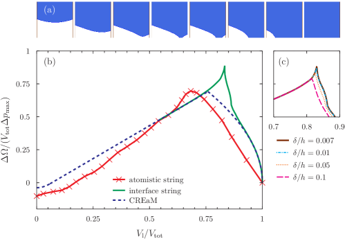
Figure 3: (a) Transition path computed via the interface string. (Multimedia view). (b) Rescaled excess free-energy along the interface string for $\Delta\tilde{p}=0$, $\alpha=1$, $\delta/h=0.0001$, $\theta_{Y}=110^{\circ}$, and $N=140$ (in green). The profile is compared to the atomistic and CREaM results at the same conditions. On the abscissa the parametric variable of the CREaM method $V_{l}/V_{tot}$ is reported; for the interface string $V_{l}/V_{tot}$ is computed from the path in the top panel, while for the atomistic string $V_{l}/V_{tot}=(Z-Z_{cassie})/(Z_{wenzel}-Z_{cassie})$, where $Z$ is the total number of particles inside the coarse-graining cells. The saddle point corresponds to a configuration where the liquid-vapor interface touches the bottom of the capillary (between image 3 and 4 of the path above). (c) Behavior of the saddle point at different $\delta/h$.

Here we discuss the relation between the wetting path identified by the continuum rare events method (CREaM) previously introduced in Giacomello et al.Giacomello et al. (2012a) and the interface “string”. We start by introducing the committor function and isocommittor surfaces. The committor is the probability that a trajectory passing by a state, an atomistic or a macroscopic configuration, will reach next the product state, say Wenzel, rather than the reactant state. An isocommittor surface is the (hyper)surface in the state space of constant committor function value. Thus, for example, the isocommittor $0.5$ is the surface of states having $50$ % of probability to reach first the products and $50$ % to reach first the reactants. This surface is, by definition, the transition state.

Consider an isocommittor surface, $S$ which intersects the MFEP at a point ${\bm{z}}(\alpha)$. Let us denote by ${\bm{n}}_{\alpha}$ the normal to $S$ at ${\bm{z}}(\alpha)$, and by ${\bm{\tau}}({\bm{z}}_{\alpha})$ the tangent to the MFEP at the same point. In Ref. Maragliano et al., 2006 it is shown that:

$${\bm{\tau}}({\bm{z}}_{\alpha})\parallel\hat{M}{\bm{n}}_{\alpha}.$$ (22)

If we compare Eq. (22) with Eq (3), we conclude that the MFEP is the path connecting constrained minima of the free-energy on the isocommittor surfaces $S_{\alpha}$ foliating the space.

Similar to the string method, CREaM aims at identifying a wetting path. However, at variance with the string method, in CREaM this path is not parametrized with its arc-length but with an observable of relevance for the problem at hand. This very general framework can be applied to different models, ranging from the micro- to the macroscale; for the macroscopic scale, in the sharp-interface model that was originally used to describe the Cassie-Wenzel transition, the wetting path is parametrized with the volume of liquid in the groove, $V_{l}$. Like in the case of the string method, in CREaM the free-energy is minimized subject to the constraint that the variable parametrizing the path is constant. In other words, the path obtained by CREaM connects the constrained minima of the free-energy on the constant volume surfaces $S^{V}_{\alpha}$.

Comparing this formulation of the CREaM path with the formulation of the string path in terms of constrained minimization of the free-energy in the isocommittor surface, we conclude that the two paths coincide if and only if $S^{V}_{\alpha}\equiv S_{\alpha}$, at least locally to the path.

In Fig. 3b we compare the CREaM and interface string free energy profiles along the respective paths. We remark that the profiles coincide for most of the path, departing from each other only in a relatively small region around the transition state. This is not surprising because, at variance with the string, CREaM does not impose the continuity of the path. Thus, in the case of the Cassie-Wentzel transition, which takes place through a morphological transition (see Ref. Giacomello et al., 2012a and Sec. V), CREaM does not map the continuous path, along which the symmetric meniscus configuration goes into the gas-bubble-in-a-corner one (see Fig. 4). In Fig. 3b we report also the free-energy profile obtained from atomistic simulations. The agreement seems to be better between atomistic and CREaM results than with interface string. The reason for this is discussed more in detail in the results section; here we remark that this better agreement is due to “errors cancellation”, with the underestimation of the barrier in CREaM compensating for an overestimation intrinsic to the sharp-interface models.

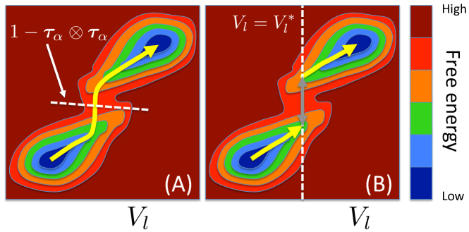
Figure 4: String (A) vs CREaM (B) paths. In this sketch one of the axis represents the volume of liquid in the cavity $V_{l}$ while the other represents the complementary degrees of freedom. The dashed line in panel (A) is the hyperplane $\left(\bm{1}-\bm{\tau}(\bm{z}(\alpha_{l},t))\otimes\bm{\tau}(\bm{z}(\alpha_{l},t))\right)\bm{v}$, where $\bm{v}$ is a generic vector. This is the plane on which $\hat{M}\nabla F$ is zero. The dashed line in panel (B), instead, represents the hypersurface $V=V_{l}$, i.e. one of the infinite hypersurfaces on which the minimum of the free energy is sought in the CREaM method. The string path follows the valley of the reactants and then moves smoothly to the valley of the products. When the reactants and products valleys become parallel, the CREaM path moves abruptly from one to the other, following the minimum of the free-energy corresponding to a given level of progress of the reaction. This is shown on the panel (B): the yellow line denotes the two branches of the CREaM path, and the gray double arrow highlights its discontinuity.

Summarizing, the paths obtained from CREaM and the string method are not identical but give the same qualitative description of the process. While the string method gives a detailed and continuous description of the most likely wetting path all along the process, CREaM represents the segment around the transition state as a sharp morphological transition (Fig. 4). Indeed, CREaM and the string can be used as complementary tools. CREaM allows to efficiently compute all the possible “reactive” channels. The string method can then be used to further refine the CREaM paths. When the system is relatively simple, like the case of wetting of a square groove, Giacomello et al. (2012a) it is possible to obtain the analytical solution of the CREaM equations. Thanks to CREaM it was possible to derive an extended version of the Laplace equation, which relates the liquid/gas meniscus curvature to the surface tension. This relation, that was introduced for the first time in Ref. Giacomello et al., 2012a, is valid along most of the wetting path, apart in the region connecting the symmetric meniscus and gas-bubble-in-a-corner morphologies. Finally, CREaM has a high parallel efficiency, even higher than the string method as it does not require any exchange of data among images, and can be run on non connected heterogeneous computers.

V Results and Discussion

In this section, we present the “physical” results obtained via the atomistic string and the sharp-interface calculations (string and CREaM) introduced in the previous sections. We focus on the transition path for the Cassie-Wenzel transition and on the related free-energy profiles. The length scales covered range from few particle diameters $\sim 11\sigma$ of the smallest atomistic system simulated to macroscopic scales, which are described in terms of sharp-interface models.

V.1 The atomistic string

The mechanism of the Cassie-Wenzel transition

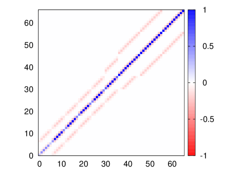
Figure 5: Metric matrix computed from Eq. (4) at image $31$ (Wenzel state). The matrix elements are normalized with the maximum value. On the $x$ and $y$ axes is reported the cell number. Values lower than one are observed on the diagonal where the density is lower than the bulk liquid one (at the wall corners, see Fig. 6).

We computed the transition path of the Cassie-Wenzel transition on two geometries, a square and a rectangular groove (Fig. 2). A total of $32$ images was used to discretize the string: the images and graphs that follow are labeled with the image number. The pressure of the NPT simulations was chosen to be close to the coexistence between the Cassie and the Wenzel states. The strings were initialized from configurations extracted from RMD simulations with a single collective variable, number of particles in the groove, analogous, apart for the ensemble (here NPT), to those presented and discussed in Ref. Giacomello et al., 2012b. We ensure that all initial images in the string have the same symmetry, that is, all menisci lie in the same corner, the left one.

A general result of the atomistic string calculations is the form of the metric matrix along the string. A representative one is reported in Fig. 5, showing that the most significant elements are those on the main diagonal. This result supports the assumption of a unitary metric matrix as is usually done in macroscopic, sharp-interface models. However, there are other very small but non-zero elements related to the surrounding coarse-graining cells as reflected by the multi-diagonal character of the metric matrix. These fine details could be encompassed in macroscopic models once the metric matrix is known from atomistic simulations. The detailed analysis of the effect of the metric matrix is deferred to a future study.

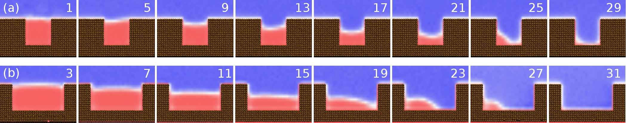
Figure 6: MFEP computed with the atomistic string method for grooves having square (a) and rectangular aspect ratios (b). The actual width of the rectangular groove is double the square one. Blue identifies high density, close to the liquid bulk one, while red low density (vapor). The image number is indicated in the corresponding density field. (Multimedia view).

The square groove measures around $11\sigma\times 11\sigma$. The thermodynamic conditions were $T=0.8$ and $P=0.001$ in LJ units, where $P$ is the global pressure observable computed for all atoms. Around $30$ steps of evolution of the string (for each of which the mean forces were computed via RMD simulations, see Sec. II.2) were required to ensure convergence.

In Fig. 6a we show the transition path for the square groove, i.e., the sequence of average density fields forming the string at convergence. The meniscus is initially flat close to the Cassie state. As the transition proceeds, the meniscus descends into the groove with constant curvature (images $7$-$21$) until close to the bottom a liquid finger is formed on the right side of the groove (images $22$-$24$). Eventually the liquid wets one corner of the groove forming a circular bubble that gradually shrinks (images $25$-$29$) until it is completely absorbed and the Wenzel state is reached (images $30$-$32$).

The initial and final parts of the path (the initial pinning, the symmetric meniscus, and the final bubble in the corner) are in fair agreement with previous restrained molecular dynamics simulations Giacomello et al. (2012b) and the macroscopic CREaM results Giacomello et al. (2012a) (see Fig. 1). However, close to the transition state the liquid-vapor interface forms a finger thus departing from the constant curvature menisci prescribed by CREaM. This discrepancy is explained by the interface string path which, close to the transition state, exhibits a point of the meniscus with high curvature (similar to the atomistic finger) that eventually touches the bottom wall creating a small and a large bubble (see Fig. 3a). The fine details of the process, however, are not easy to compare, because the diffuse nature of the atomistic interface tends to smear out sharp points and small vapor domains; to this must be added that computational constraints limit the number of images and coarse-graining cells in the atomistic string.

The rectangular groove measures around $22\sigma\times 11\sigma$ and is therefore twice as wide as the square one. The thermodynamic conditions of the NPT simulations were $T=0.8$ and $P=0$ for this case. More than $30$ steps of string evolution were required for convergence.

The MFEP for the rectangular groove is shown in Fig. 6b. It is seen that before the Cassie minimum the meniscus curvature is allowed to vary while the triple line is pinned at the top corners of the groove (images $1$-$5$), as is expected from the macroscopic Gibbs’ criterion Oliver, Huh, and Mason (1977). This is an evidence that pinning happens also at the nanoscale, even though in a particle description of the system the continuum concept of “geometrical singularity” (corners at the top of the groove, in the present case) has no meaning. However, the string resolution (number of images) does not allow us to quantify the range of contact angles for which pinning occurs. The intrusion into the groove happens when a sufficiently large meniscus curvature is reached, around image $5$. The meniscus bends towards one corner at images $14$-$17$, earlier in the progress of the transition than in the case of the square groove. This observation can be made more quantitative by considering the length of the string up to the transition state and normalizing it with the total length of the string concerned with the activated event, that is, $\alpha_{TS}=(i_{TS}-i_{\mathrm{cassie}}-1)/(i_{\mathrm{wenzel}}-i_{\mathrm{cassie}}-1)$, where $i$ is the image number; for the rectangular groove $\alpha_{TS}=14/26$, while for the square one $\alpha_{TS}=19/26$. The contact line touches the bottom wall (on the right hand side) and recedes “rapidly” towards the opposite corner while the contact line at the vertical wall on the left does not move. As a consequence, during the shrinking process the bubble at the corner starts with a slightly flattened shape and then tends to a circular one. This mechanism seems a generic one for the contact with the wall, since the interface string path for the square groove also shows that the left contact line behaves as if it were “pinned” at the vertical wall – although there is no defect – while the right contact line slides on the bottom wall (see Fig. 3a).

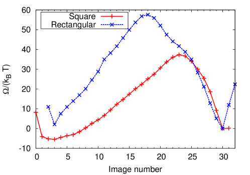
Figure 7: Free-energy profiles related to the MFEPs shown in Fig. 6 in $k_{B}T$ units. The square groove is at $P=0.001$ and the rectangular groove at $P=0$. The image count for the rectangular groove is shifted by $+2$ in order to make the two Wenzel states coincide. The reference free-energy is taken to be that relative to the Wenzel state, $\Omega_{W}\equiv 0$.

The free-energy profiles related to the MFEPs just presented are shown in Fig. 7. We remind that the profiles are at slightly different pressures. In both cases, the free-energy barriers connected to the Cassie-Wenzel transition are large as compared to the thermal energy $k_{B}T$, a fact that corroborates the presence of strong metastabilities on nano-rough hydrophobic surfaces. The free-energy barrier for the square groove is $34.3$ $k_{B}T$, while for the rectangular one is $44.3$ $k_{B}T$, around $30\%$ larger, suggesting that both the size and the aspect ratio of the groove have an effect on the kinetics of the Cassie-Wenzel transition.

Validity of the concept of transition path

In Fig. 8 we show atomistic configurations extracted from the transition state ensemble of the square groove; these microstates were computed via RMD as detailed in Sec. II.3. It is apparent that the microscopic configurations correspond to several macroscopic states: bubble on the right corner, on the left one, and in the center. For the larger rectangular groove, instead, the transition state ensemble is connected with a well defined configuration featuring a bubble in the left corner, similar to that shown in Fig. 6b (see also the related movie).

We ascribe this behavior to the flat free-energy landscape along the hyperplane orthogonal to the transition state. When the barrier separating the symmetry-related wetting paths (bubble-on-the-left and bubble-on-the-right corners) is $\leq k_{B}T$ the system can easily jump from one to the other. In this case, the wetting path identified by the string (and CREaM) method has little statistical significance. In other words, the transition tubes Maragliano et al. (2006); Vanden-Eijnden (2006) around the two specular paths, i.e., the region of state space in which most of the transition trajectories pass through, overlap. Thus, we cannot describe the wetting trajectories as “fluctuations” around the MFEP. In these conditions, other methods, such as the finite temperature string E, Ren, and Vanden-Eijnden (2005), would be needed to capture information about the transition.

These results suggest that the macroscopic models of capillary systems have a lower length scale below which they break down: the free-energy landscape becomes too flat to identify a single macroscopic state. In the language of transition path theory, for sufficiently small grooves the transition tube becomes large and the single transition path found in the zero temperature limit has no statistical significance.

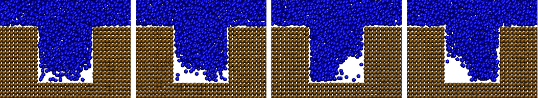
Figure 8: Atomistic configurations extracted from the transition state ensemble for the square nano-groove. (Multimedia view).

V.2 The transition state

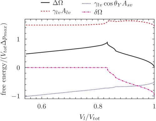
Figure 9: Contributions to the excess free-energy $\Delta\Omega$ rescaled by $V_{tot}\Delta p_{max}$. The energetic costs of forming liquid-vapor or solid-vapor interfaces and of wetting the bottom wall are defined in Eqs. (9) and (14), respectively. The results are computed via the interface string with $\Delta\tilde{p}=0$, $\alpha=1$, $\delta/h=0.0001$, $\theta_{Y}=110^{\circ}$, and $N=140$.

The interface string calculations were performed for the square groove in the region of the transition state (the maximum of the profile), which is critical both for evaluating the free-energy barriers and for testing the CREaM results. As shown by the free-energy profiles in Fig. 3b at low filling levels ($V_{l}/V_{tot}<0.75$) and high ones ($V_{l}/V_{tot}>0.9$) the interface string coincides with CREaM. Around the transition state, instead, the interface string significantly departs from CREaM. The transition state itself coincides with a cusp in the free-energy profile, while in CREaM it is a non-differentiable point (see Fig. 1). Ironically, the jump discontinuity in the derivative at the transition state found with CREaM induced us to further investigate the phenomenon, which is actually more severe in the full-fledged string which shows an infinite discontinuity of the derivative (in the sharp-interface limit $\delta\to 0$). The interface string however guarantees the continuity of the transition path, which is consistent with a continuous dynamics. The cusp arises because in touching the bottom wall the radius of curvature of the meniscus has to change sign from positive (symmetric meniscus) to negative (asymmetric bubble). This is realized with a single point of zero radius of curvature (and infinite curvature) developing on a side of the liquid-vapor interface just before the contact with the bottom wall (see Fig. 3a). A different point of view is that the area of the liquid-vapor interface significantly increases during the formation of the liquid “finger” while $V_{l}$ remains almost constant, thus giving rise to the sharp increase of the free-energy at the transition state as clearly shown by the energy balance in Fig. 9. The thermodynamic force $\mu$ corresponding to the finger becomes infinite at the transition state. This divergence of $\mu$ is integrable, thus giving rise to the cusp in the free-energy profile of Fig. 3b.

In all cases analyzed – atomistic, interface string, and CREaM – the transition state is connected with the contact of the liquid domain with the bottom wall of the groove (compare the paths in Figs. 6, 3a, and 1 with the free free-energy profiles in Figs. 3b): while the meniscus descends symmetrically in the groove, the free-energy grows steadily because of the substitution of vapor-solid interface with liquid-solid one which is unfavorable for hydrophobic materials (see Fig. 9); when contact of the meniscus with the bottom wall eventually occurs, new liquid-solid interface replaces the liquid-vapor and solid-vapor interfaces at the bottom, resulting in an overall reduction of the free-energy (the negative term $\delta\Omega$ in Fig. 9).

In the atomistic string, the transition state is found around one-half of the string for the rectangular groove while it is towards the end of it for the square one (see Fig. 7). The location of the transition thus depends on the aspect ratio of the groove; this fact is easily explained by the balance of the energy contributions above: for a taller groove the (growing) branch of the free-energy connected with the meniscus sliding on the vertical walls of the groove is longer, while the descending branch due to the shrinking bubble is steeper.

The atomistic free-energy profiles reported in Fig. 7 are smooth at the transition state, differently from those obtained via the interface string and via CREaM (see Fig. 3b). In the atomistic case, indeed, thermal fluctuations tend to smear out the extreme events seen in the sharp-interface models. In particular, the formation of a point in the meniscus with very high curvature is impossible in an atomistic picture. In order to account for this effect, we repeat the interface string calculations at increasing values of $\delta$, which correspond to wider liquid-vapor interfaces, see Fig. 3c. The case $\delta/h=0.1$ roughly corresponds to the atomistic one, where the ratio of the interface thickness and the groove width is also $\sim 0.1$. Figure 3c demonstrates that in the case of diffuse interfaces the transition state is smooth and the height of the free-energy barrier tends to decrease.

VI Conclusions

The atomistic string method in the density field collective variable was applied for the first time to the Cassie-Wenzel transition to determine rigorously the mechanism of the transition. The results of this work are both methodological and physical. From the methodological point of view, we demonstrated the relationship between approximate macroscopic methodsGiacomello et al. (2012a) and the full-fledged interface string. The former methods are algorithmically simple and computationally convenient but fail where more parallel valleys are present in the free-energy landscape.

The string simulations also offered physical insight into the mechanism of the Cassie-Wenzel transition from the nanoscale to the macroscale. A morphological transition was observed during the rare event with the meniscus changing from a symmetric to an asymmetric configuration. The contact of the meniscus with the bottom wall determines the position and shape of the transition state; at the nanoscale the transition state is smooth, while in macroscopic models it shows a cusp-like behavior. The free-energy barriers are large compared to $k_{B}T$ even in nanoscale grooves; the depth of the groove and its aspect ratio are the critical parameters to determine the kinetics of the Cassie-Wenzel transition. It was also shown that for very small grooves (width $\sim 11\sigma$) the concept of transition path breaks down and it is not possible to identify a unique sequence of macroscopic configurations that describe the Cassie-Wenzel transition.