Generation of large-scale magnetic fields, non-Gaussianity, and primordial gravitational waves in inflationary cosmology

Abstract

The generation of large-scale magnetic fields in inflationary cosmology is explored, in particular, in a kind of moduli inflation motivated by racetrack inflation in the context of the Type IIB string theory. In this model, the conformal invariance of the hypercharge electromagnetic fields is broken thanks to the coupling of both the scalar and pseudoscalar fields to the hypercharge electromagnetic fields. The following three cosmological observable quantities are first evaluated: The current magnetic field strength on the Hubble horizon scale, which is much smaller than the upper limit from the back reaction problem, local non-Gaussianity of the curvature perturbations due to the existence of the massive gauge fields, and the tensor-to-scalar ratio. It is explicitly demonstrated that the resultant values of local non-Gaussianity and the tensor-to-scalar ratio are consistent with the Planck data.

OCHA-PP-330

I Introduction

It is observationally confirmed that there are galactic magnetic fields on $1$–$10$kpc scale with the strength of $\sim 10^{-6}$G, and that also in clusters of galaxies, there exist the magnetic fields on $10$ kpc–$1$Mpc scale with their amplitude of $10^{-7}$–$10^{-6}$G. The origins of cosmic magnetic fields, particularly, such large-scale magnetic fields in clusters of galaxies have not yet been established (for reviews, see, e.g., M-F-Reviews ). There have been proposed various generation mechanisms such as the plasma instability Biermann1 ; PI , cosmological electroweak and quark-hadron phase transitions PT , cosmic string M-CS , primordial density perturbations DP , and the secondary dynamo amplification mechanism EParker . However, it is difficult for these mechanism to produce the large-scale magnetic fields.

It is known that electromagnetic quantum fluctuations generated during inflation are the most natural origin of large-scale magnetic fields Inflation , because the coherent scale of magnetic fields can be extended larger than the Hubble horizon at the inflationary stage Turner:1987bw . The Maxwell theory has its conformal invariance. Moreover, the Friedmann-Lemaître-Robertson-Walker (FLRW) metric, which describes the homogeneous and isotropic universe consistent with observations, is conformally flat. Hence, at the inflationary stage, the conformal invariance of the electromagnetic fields has to be broken so that the quantum fluctuations of the electromagnetic fields can be generated Parker:1968mv and eventually result in the large-scale magnetic fields at the present time Turner:1987bw ; N-G-C . There are several well-known ideas of the breaking mechanism: e.g., ($i$) A non-minimal coupling between the scalar curvature and the electromagnetic fields produced by a one-loop vacuum-polarization effect in quantum electrodynamics in the curved space-time Drummond:1979pp ; ($ii$) A coupling of a scalar field to the electromagnetic fields Ratra:1991bn ; MF-Scalar ; B-Y ; Garretson:1992vt ; ($iii$) The trace anomaly Dolgov:1993vg .

In this paper, we investigate the generation of large-scale magnetic fields from a kind of moduli inflation inspired by racetrack inflation BlancoPillado:2004ns in the framework of the Type IIB string theory with the so-called Kachru-Kallosh-Linde-Trivedi volume stabilization mechanism Kachru:2003aw . In this model, the conformal invariance of the hypercharge electromagnetic fields is broken through their coupling to both a scalar field and an axion-like pseudoscalar one. It should be noted that our model is still a toy model motivated by racetrack inflation or so-called axion inflation, where the axion plays a role of the inflaton. The main purpose of this work is that by using a simple model, we reveal cosmological consequences in racetrack (or axion) inflation. In Refs. Barnaby:2010vf ; Barnaby:2011vw , it has been indicated that a coupling of the pseudoscalar inflaton field to the electromagnetic fields can generate non-Gaussianity Komatsu:2001rj ; Tanaka:2010km of power spectrum of the curvature perturbations coming from the quantum fluctuations of the inflaton field. Thus, we analyze non-Gaussianity of the curvature perturbations in the present scenario by following the procedure in Refs. Meerburg:2012id ; Linde:2012bt . Moreover, we study the so-called tensor-to-scalar ratio defined by the ratio of scalar modes of the curvature perturbations to their tensor modes (namely, the primordial gravitational waves) Barnaby:2011qe ; Barnaby:2012xt . We show that if the magnetic fields on the Hubble horizon scale with their current strength compatible with the back reaction problem are generated, local non-Gaussianity and the tensor-to-scalar ratio in the cosmic microwave background (CMB) radiation with those values smaller than the limits from the Planck satellite Ade:2013ydc can be produced. The most important result of this work is that the explicit values of three cosmological observable quantities, i.e., the large-scale magnetic fields, local non-Gaussianity, and the tensor-to-scalar ratio are first derived. Furthermore, we should emphasize the novelty of our present model in comparison with the other recent works on non-Gaussianity of the curvature perturbations and the tensor-to-scalar ratio in a kind of axion inflation Meerburg:2012id ; Linde:2012bt ; Bugaev:2013fya ; Barnaby:2010vf ; Barnaby:2011vw . In our model, a scalar field as well as the axion-like pseudoscalar field couple to the hypercharge electromagnetic field, whereas in the other past models, only the pseudoscalar field couples to the hypercharge electromagnetic field. The existence of such a scalar field coupling to the (hypercharge) electromagnetic field is suggested by the Kaluza-Klein (KK) compactification mechanism K-K for the fundamental higher-dimensional space-time theories including string theories. In fact, both couplings appears in the framework of racetrack inflation. Thus, the setting of our model is closer to the realistic one than that in the past related works, although it is a toy model. In addition, there is one more significant advantage that thanks to the coupling of the scalar filed to the hypercharge electromagnetic field, in principle, the large-scale magnetic fields with the current strength enough to explain the observations without any secondary amplification mechanism like the galactic dynamo. This point cannot be realized in the past models.

The observational test of this model is the severest, therefore it is very difficult for the model to be viable, because we use the three independent observations of the large-scale magnetic fields, local non-Gaussianity, and tensor-to-scalar ratio. Furthermore, this model is the most general within the fundamental theories which we are considering. Thus, we develop the generic discussions in order not only to extend the theoretical possibility but also to strictly constrain the freedom of the theory. We use the units $k_{\mathrm{B}}=c=\hbar=1$ and describe the Newton’s constant by $G=1/M_{\mathrm{P}}^{2}$, where $M_{\mathrm{P}}=2.43\times 10^{18}$ GeV is the reduced Planck mass. In terms of electromagnetism, we adopt Heaviside-Lorentz units.

The paper is organized as follows. In Sec. II, we explain our model action and derive the basic equations. In Sec. III, we investigate the evolution of each field and estimate the current strength of the large-scale magnetic fields. In Sec. IV, we explore the power spectrum of the curvature perturbations, non-Gaussianity, and the tensor-to-scalar ratio. In Sec. V, conclusions are presented. In Appendix A, we examine the large-scale magnetic fields, non-Gaussianity, and tensor-to-scalar ratio for the axion (monodromy) inflation, and comparison these results with the ones for a kind of moduli inflation motivated by racetrack inflation in the previous sections. In Appendix B, the issues of the backreaction and the strong coupling are stated. In Appendix C, the observational constraints on the field strength of magnetic fields are summarized. Cosmological implications related to this work are also stated in Appendix D.

II Model

Our model Lagrangian is given by

$${\mathcal{L}} = \frac{M_{\mathrm{P}}^{2}}{2}R-\frac{1}{4}XF_{\mu\nu}F^{\mu\nu}-\frac{1}{4}g_{\mathrm{ps}}\frac{Y}{M}F_{\mu\nu}\tilde{F}^{\mu\nu}$$ (1)

$${}-\frac{1}{2}g^{\mu\nu}{\partial}_{\mu}{\Phi}{\partial}_{\nu}{\Phi}-U(\Phi)-\frac{1}{2}g^{\mu\nu}{\partial}_{\mu}{Y}{\partial}_{\nu}{Y}-V(Y)\,,$$

$$X \equiv \exp\left(-\lambda\frac{\Phi}{M_{P}}\right)\,,$$ (2)

$$V(Y)\approx\bar{V}-\frac{1}{2}m^{2}Y^{2}\,,$$ (3)

where $R$ is the Ricci scalar, $g_{\mathrm{ps}}$ is a dimensionless coupling constant, $\Phi$ is the canonically normalized field of the scalar field $X$ with the normalization constant $\lambda$, $Y$ is a canonical pseudoscalar field, and $M$ is a constant with the dimension of mass corresponding to the decay constant of $Y$. Furthermore, $F_{\mu\nu}=\nabla_{\mu}F_{\nu}-\nabla_{\nu}F_{\mu}$ is the field strength of the $\mathrm{U}(1)_{Y}$ hypercharge gauge field $F_{\mu}$, where $\nabla_{\mu}$ is the covariant derivative, and $\tilde{F}^{\mu\nu}$ are the dual field strength of $F_{\mu}$. While we do not specify the exact form of scalar potentials $U(X=X(\Phi))$, $Y$ would be expected to have a potential, given by Eq. (3) with a normalization factor $\bar{V}$ and the mass $m$ of the pseudoscalar $Y$. The pseudoscalar field $Y$ couples to the dual of the field strength, and hence it acts as an axion. Throughout our analysis, we assume that inflation is driven by the potential energy of $Y$ as in the so-called natural inflation or axion inflation Anber:2009ua ; N-A-I ; CN-inflation . We take the flat FLRW space-time

$${ds}^{2}=-{dt}^{2}+a^{2}(t)d{\mbox{\boldmath$x$}}^{2}\,,$$ (4)

with $a$ the scale factor. In this background, the field equations of $\Phi$ (i.e., $X$) and $Y$ read

$$\ddot{\Phi}+3H\dot{\Phi}+\frac{dU(\Phi)}{d\Phi}=0\,,\quad\ddot{Y}+3H\dot{Y}+\frac{dV(Y)}{dY}=0\,,$$ (5)

where $H\equiv\dot{a}/a$ is the Hubble parameter and the dot denotes the derivative with respect to the cosmic time $t$. Using the Coulomb gauge $F_{0}(t,\mbox{\boldmath$x$})=0$ and ${\partial}_{j}F^{j}(t,\mbox{\boldmath$x$})=0$, we find that the field equation of $F_{\mu}$ is described as

$$\ddot{F_{i}}(t,\mbox{\boldmath$x$})+\left(H+\frac{\dot{X}}{X}\right)\dot{F_{i}}(t,\mbox{\boldmath$x$})-\frac{1}{a^{2}}{\partial}_{j}{\partial}_{j}F_{i}(t,\mbox{\boldmath$x$})-\frac{g_{\mathrm{ps}}}{M}\frac{1}{aX}\dot{Y}\epsilon^{ijk}{\partial}_{j}F_{k}(t,\mbox{\boldmath$x$})=0\,,$$ (6)

where the second term within the round bracket $(\,)$ and the fourth term originate from the breaking of the conformal invariance of the hypercharge electromagnetic fields.

III Current strength of large-scale magnetic fields

In this section, we explore the evolutions of the $\mathrm{U}(1)_{Y}$ gauge field, the scalar field $X$, and the pseudoscalar field $Y$, and estimate the strength of large-scale magnetic fields at the present time.

III.1 Scalar and pseudoscalar fields

We suppose that inflation is basically driven by the potential of $Y$. In the FLRW background (4), the Friedmann equation becomes $3M_{\mathrm{P}}H^{2}=\left[\left(1/2\right){\dot{Y}}^{2}+V(Y)\right]$. If the so-called slow-roll approximation $\dot{Y}^{2}/2\ll V(Y)$ is satisfied, we have $H\approx H_{\mathrm{inf}}=\mathrm{constant}$ with $H_{\mathrm{inf}}$ the Hubble parameter during inflation, so that the exponential inflation can be realized. In this case, the scale factor $a(t)$ can be expressed as $a(t)=a_{k}\exp\left[H_{\mathrm{inf}}\left(t-t_{k}\right)\right]$ with $a_{k}=a(t_{k})$, where $t_{k}$ is the time when a comoving wavelength $2\pi/k$ of the $\mathrm{U}(1)_{Y}$ gauge field first crosses the horizon at the inflationary stage, and thus $k/(a_{k}H_{\mathrm{inf}})=1$ is met. The analytic solution of Eq. (5) is given by Garretson:1992vt

$$Y=Y_{k}\exp\left\{\frac{3}{2}\left[-1\pm\sqrt{1+\left(\frac{2m}{3H_{\mathrm{inf}}}\right)^{2}}\right]H_{\mathrm{inf}}\left(t-t_{k}\right)\right\}\,,$$ (7)

with $Y_{k}=Y(t_{k})$. In the following, we use this solution. In particular, without generality, we take the “$+$” sign on the right-hand side of this solution. On the other hand, regarding $X$, we study the case that the concrete dynamics of $X$ during inflation does not influence on the results and only the difference between the initial and final values during inflation is important.

III.2 $\mathrm{U}(1)_{Y}$ gauge field

III.2.1 Quantization

First, we quantize the $\mathrm{U}(1)_{Y}$ gauge field $F_{\mu}(t,\mbox{\boldmath$x$})$. It follows from the hypercharge electromagnetic part of the action constructed by the Lagrangian (1), we find that the canonical momenta conjugate to $F_{\mu}(t,\mbox{\boldmath$x$})$ read ${\pi}_{0}=0$ and ${\pi}_{i}=Xa\dot{F_{i}}(t,\mbox{\boldmath$x$})$. The canonical commutation relation between $F_{i}(t,\mbox{\boldmath$x$})$ and ${\pi}_{j}(t,\mbox{\boldmath$x$})$ is imposed as

$$\left[F_{i}(t,\mbox{\boldmath$x$}),{\pi}_{j}(t,\mbox{\boldmath$y$})\right]=i\int\frac{d^{3}k}{(2\pi)^{3/2}}\mathrm{e}^{i\mbox{\boldmath\tiny$k$}\cdot\left(\mbox{\boldmath\tiny$x$}-\mbox{\boldmath\tiny$y$}\right)}\left[{\delta}_{ij}-\left(k_{i}k_{j}/k^{2}\right)\right]\,.$$ (8)

Here, $k$ is the comoving wave number and its amplitude is expressed as $k=|\mbox{\boldmath$k$}|$. This relation leads to the description of $F_{i}(t,\mbox{\boldmath$x$})$ as

$$F_{i}(t,\mbox{\boldmath$x$})=\int\frac{d^{3}k}{(2\pi)^{3/2}}\left[\hat{b}(\mbox{\boldmath$k$})F_{i}(t,\mbox{\boldmath$k$})\mathrm{e}^{i\mbox{\boldmath\tiny$k$}\cdot\mbox{\boldmath\tiny$x$}}+{\hat{b}}^{\dagger}(\mbox{\boldmath$k$}){F_{i}^{*}}(t,\mbox{\boldmath$k$})\mathrm{e}^{-i\mbox{\boldmath\tiny$k$}\cdot\mbox{\boldmath\tiny$x$}}\right]\,,$$ (9)

where $\hat{b}(\mbox{\boldmath$k$})$ and ${\hat{b}}^{\dagger}(\mbox{\boldmath$k$})$ are the annihilation and creation operators, respectively. These operators obey the relations

$$\left[\hat{b}(\mbox{\boldmath$k$}),{\hat{b}}^{\dagger}({\mbox{\boldmath$k$}}^{\prime})\right]={\delta}^{3}(\mbox{\boldmath$k$}-{\mbox{\boldmath$k$}}^{\prime})\,,\quad\left[\hat{b}(\mbox{\boldmath$k$}),\hat{b}({\mbox{\boldmath$k$}}^{\prime})\right]=\left[{\hat{b}}^{\dagger}(\mbox{\boldmath$k$}),{\hat{b}}^{\dagger}({\mbox{\boldmath$k$}}^{\prime})\right]=0\,.$$ (10)

We also have the normalization condition as

$$F_{i}(k,t){\dot{F}}_{j}^{*}(k,t)-{\dot{F}}_{j}(k,t){F_{i}^{*}}(k,t)=\frac{i}{Xa}\left[{\delta}_{ij}-\left(k_{i}k_{j}/k^{2}\right)\right]\,.$$ (11)

III.2.2 Set up

We set the $x^{3}$ axis to lie along the direction of the spatial momentum $k$ and express the transverse directions as $x^{1}$ and $x^{2}$. By using Eq. (6) and defining the circular polarizations $F_{\pm}(k,t)\equiv F_{1}(k,t)\pm iF_{2}(k,t)$ with the Fourier modes $F_{1}(k,t)$ and $F_{2}(k,t)$ of the $\mathrm{U}(1)_{Y}$ gauge field, we acquire

$$\ddot{F}_{\pm}(k,t)+\left(H_{\mathrm{inf}}+\frac{\dot{X}}{X}\right)\dot{F}_{\pm}(k,t)+\left[1\pm\frac{g_{\mathrm{ps}}}{M}\frac{\dot{Y}}{X}\left(\frac{k}{a}\right)^{-1}\right]\left(\frac{k}{a}\right)^{2}F_{\pm}(k,t)=0\,,$$ (12)

During inflation, we numerically solve this equation by following the procedure in Ref. Bamba:2006km , because it is very hard to acquire the analytic solution of Eq. (12). For the sub-horizon scale $k/\left(aH\right)\gg 1$, the $F_{-}(k,t)$ corresponds to the decaying mode, and therefore we only examine the evolution of $F_{+}(k,t)$.

An approximate amplitude $F_{+}(k,t=t_{k})$ at the horizon crossing, where $k/\left(aH_{\mathrm{inf}}\right)=1$, is represented as Barnaby:2010vf ; Barnaby:2011vw ; Anber:2009ua $F_{+}(k,t_{k})\simeq\left(1/\sqrt{2k}\right)\left(1/\sqrt{X(t_{k})}\right)\left(2\xi_{k}\right)^{-1/4}\exp\left(\pi\xi_{k}-2\sqrt{2\xi_{k}}\right)$ with $\xi_{k}=\xi(t=t_{k})$. Here,

$$\xi\equiv\frac{1}{2}\frac{g_{\mathrm{ps}}}{M}\frac{1}{X}\frac{\dot{Y}}{H_{\mathrm{inf}}}\,.$$ (13)

This amplification comes from the tachyonic instability. Thus, when we numerically calculate Eq. (12), we take into account the above amplification factor in the initial conditions. We define the following amplification factor as

$$C_{+}(k,t)\equiv\frac{F_{+}(k,t)}{F_{+}(k,t_{k})}\,.$$ (14)

We estimate the initial amplitude of $F_{+}(k,t)$, i.e., $F_{+}(k,t_{k})$, by matching with the solution for sub-horizon scales $k/(aH)\gg 1$ at the horizon exit Bamba:2006km . Here, we assume that in the short-wavelength limit of $k\rightarrow\infty$, the amplitude of $F_{+}(k,t)$ is described by $\left|F_{+}^{(\mathrm{in})}(k,t)\right|=\left(1/\sqrt{2k}\right)\left(1/\sqrt{X(t)}\right)$, where the coefficients of modes have been chosen so that the vacuum can be reduced to the one in the Minkowski space-time in the short-wavelength limit (the so-called Bunch-Davies vacuum B-D ).

III.2.3 Numerical analysis

We derive the strength of large-scale magnetic fields, provided that during inflation, $X$ can approximately be regarded as a constant. This means that a dynamical quantity to the hypercharge electromagnetic fields is only the pseudoscalar field $Y$. Such a case has been explored in Refs. Garretson:1992vt ; Barnaby:2010vf ; Barnaby:2011vw ; Barnaby:2011qe ; Pajer:2013fsa . Indeed, the field strength of the large-scale magnetic fields can be amplified in our model, where the hypercharge electromagnetic fields couple to the scalar field $X$. In other words, the important quantity to characterize the amplification of the magnetic fields is the ratio of the final value of $X$ to the initial one at inflationary stage. The ordinary theory of the electromagnetic fields, where $X=1$, has to be recovered by the epoch of the Big Bang Nucleosynthesis (BBN). Accordingly, we suppose that $X$ stays almost constant during inflation, and after inflation it quickly reaches $X(t=t_{\mathrm{R}})=1$ at the reheating stage $t_{R}$ owing to an appropriate form of $V(\Phi)$.

Figure 1: $C_{+}(k,t)$ as a function of $H_{\mathrm{inf}}t$ for $X(t_{k})\equiv\exp\left(\chi_{k}\right)$ with $\chi_{k}=-0.940$, $H_{\mathrm{inf}}=1.0\times 10^{10}$GeV, $m=2.44\times 10^{9}$GeV, $Y_{k}=7.70\times 10^{-2}M_{\mathrm{P}}=1.87\times 10^{17}\,\mathrm{GeV}$, $M=1.0\times 10^{-1}M_{\mathrm{P}}=2.43\times 10^{17}\,\mathrm{GeV}$, $\bar{V}=5.07\times 10^{-17}M_{\mathrm{P}}^{4}$, $\xi_{k}=2.5590616$, and $g_{\mathrm{ps}}=1.0$ (the case (b) in Table 1). The solid line shows the case including the dynamics of $Y$, whereas the dotted line depicts that without it, namely, $\dot{Y}=0$ in Eq. (12).

In Fig. 1, we depict the evolution of $C_{+}(k,t)$ during inflation with the solid line for $X(t_{k})\equiv\exp\left(\chi_{k}\right)$ with $\chi_{k}=-0.940$, $H_{\mathrm{inf}}=1.0\times 10^{10}$GeV, $m=2.44\times 10^{9}$GeV, $M=1.0\times 10^{-1}M_{\mathrm{P}}=2.43\times 10^{17}\,\mathrm{GeV}$, $\bar{V}=5.07\times 10^{-17}M_{\mathrm{P}}^{4}$, $\xi_{k}=2.5590616$, and $g_{\mathrm{ps}}=1.0$. This is the case (b) in Table 1 shown later. We have numerically solved Eq. (12) for $k=a_{k}H_{\mathrm{inf}}$ mode for the exponential inflation from the initial time at $t=t_{k}=H_{\mathrm{inf}}^{-1}$, when we set $C_{+}(k,t_{k})=1$. We define the values of these parameters by the Cosmic Background Explorer (COBE) Smoot:1992td normalization and Planck data Ade:2013uln on the CMB radiation. For comparison, we have also plotted the numerical results for the case that $\dot{Y}=0$ in Eq. (12) with the dotted line. Here, the behavior for $\dot{Y}\neq 0$ is quite similar to that for $\dot{Y}=0$, because the pseudoscalar field $Y$ rolls down its potential very slowly.

From Fig. 1, we see that $C_{+}(k,t)$ asymptotically approaches a constant within about 10 Hubble expansion time after the horizon crossing during inflation. This is an important feature of evolution of $C_{+}(k,t)$, that is, the amplitude becomes a finite value and does not decay. It contributes to the resultant strength of the large-scale magnetic fields. Such a behavior of $C_{+}(k,t)$ does not depend on the model parameters. This result is also consistent with that in Ref. Barnaby:2010vf . The way of determining the values of $m$ and $Y_{k}$ are explained in the last paragraph of Sec. IV A.

III.3 Current magnetic field strength

Next, we evaluate the magnetic field strength at the present time. The proper hypermagnetic and hyperelectric fields are represented with the comoving hypermagnetic fields ${B_{Y}}_{i}(t,\mbox{\boldmath$x$})$ and hyperelectric ones ${E_{Y}}_{i}(t,\mbox{\boldmath$x$})$, respectively, as Ratra:1991bn

$${B_{Y}}_{i}^{\mathrm{proper}}(t,\mbox{\boldmath$x$}) = \frac{1}{a^{2}}{B_{Y}}_{i}(t,\mbox{\boldmath$x$})=\frac{1}{a^{2}}{\epsilon}_{ijk}{\partial}_{j}F_{k}(t,\mbox{\boldmath$x$})\,,$$ (15)

$${E_{Y}}_{i}^{\mathrm{proper}}(t,\mbox{\boldmath$x$}) = a^{-1}{E_{Y}}_{i}(t,\mbox{\boldmath$x$})=-a^{-1}\dot{F}_{i}(t,\mbox{\boldmath$x$})\,,$$ (16)

where ${\epsilon}_{ijk}$ is the totally antisymmetric tensor (${\epsilon}_{123}=1$). Multiplying the energy density of the proper hypermagnetic field in the Fourier space ${\rho}_{B_{Y}}(k,t)$ by the phase-space density $4\pi k^{3}/(2\pi)^{3}$, we obtain the energy density of the proper hypermagnetic field in the physical space

$${\rho}_{B_{Y}}(L,t)=\frac{k^{3}}{4{\pi}^{2}}\left[\left|{B_{Y}}_{+}^{\mathrm{proper}}(k,t)\right|^{2}+\left|{B_{Y}}_{-}^{\mathrm{proper}}(k,t)\right|^{2}\right]X\,.$$ (17)

Here, $\left|{B_{Y}}_{\pm}^{\mathrm{proper}}(k,t)\right|^{2}=\left(1/a^{2}\right)\left(k/a\right)^{2}|F_{\pm}(k,t)|^{2}$, which follows from Eq. (15), and $L=2\pi/k$ is a comoving scale.

The instantaneous reheating at $t=t_{\mathrm{R}}$ after inflation occurs much earlier than the electroweak phase transition (EWPT) at $T_{\mathrm{EW}}\sim 100$GeV. The conductivity of the universe ${\sigma}_{\mathrm{c}}$ should be very small at the inflationary stage, because few particle present. In the reheating process, charged particles are created, and therefore ${\sigma}_{\mathrm{c}}$ increases and would become large enough as $(t\geq t_{\mathrm{R}})$. Hence, when ${\sigma}_{\mathrm{c}}\gg H$, the hyperelectric fields dissipate by accelerating the charged particles. In the following radiation- and matter-dominated stages $(t\geq t_{\mathrm{R}})$, we have $B_{Y}\propto a^{-2}$ Ratra:1991bn ; B-Y . Thus, at a later time after the EWPT when $X$ reached the true minimum of $X=1$, the energy density of the hypermagnetic fields $\rho_{B_{Y}}(L,t)$ reduces to that of the magnetic fields $\rho_{B}(L,t)$. The expression of $\rho_{B}(L,t)$ is given by Bamba:2006km

$$\rho_{B}(L,t)\simeq\frac{1}{8\pi^{2}}\frac{1}{X(t_{k})}\frac{1}{\sqrt{2\xi_{k}}}\exp\left[2\left(\pi\xi_{k}-2\sqrt{2\xi_{k}}\right)\right]\left(\frac{k}{a}\right)^{4}|C_{+}(k,t_{\mathrm{R}})|^{2}\,,$$ (18)

where we have imposed $X(t_{\rm R})=1$ and neglected the different coefficient factor between the magnetic field of $\mathrm{U}(1)_{Y}$ and that of $\mathrm{U}(1)_{\rm em}$ because it is order of unity.

Table 1: Current strength of magnetic fields on the Hubble horizon scale and $1$Mpc scale for $X(t_{k})=\exp\left(\chi_{k}\right)$ with $\chi_{k}=-0.940$, $M=1.0\times 10^{-1}M_{\mathrm{P}}=2.43\times 10^{17}\,\mathrm{GeV}$, $g_{\mathrm{ps}}=1.0$, $\xi_{k}=2.5590616$, and $k=2\pi/\left(2997.9h^{-1}\right)\,{\mathrm{Mpc}}^{-1}$ with $h=0.673$. For the cases (i) (i=a, b, c, d, e, f), we have $T_{\mathrm{R}}\,[\mathrm{GeV}]=(1.02\times 10^{14},\,3.22\times 10^{13},\,3.22\times 10^{12},\,3.22\times 10^{11},\,3.22\times 10^{10},\,3.22\times 10^{9})$ and $\bar{V}/M_{\mathrm{P}}^{4}=(5.07\times 10^{-15},\,5.07\times 10^{-17},\,5.07\times 10^{-21},\,5.07\times 10^{-25},\,5.07\times 10^{-29},\,5.07\times 10^{-33})$.

	$B(H_{0}^{-1},t_{0})\hskip 2.84526pt[\mathrm{G}]$	$B(1\mathrm{Mpc},t_{0})\hskip 2.84526pt[\mathrm{G}]$	$H_{\mathrm{inf}}\hskip 2.84526pt[\mathrm{GeV}]$	$m\hskip 2.84526pt[\mathrm{GeV}]$	$Y_{k}/M_{\mathrm{P}}$	$C_{+}(k,t_{\mathrm{R}})$
(a)	$7.15\times 10^{-64}$	$1.42\times 10^{-56}$	$1.0\times 10^{11}$	$2.44\times 10^{10}$	$7.70\times 10^{-2}$	$0.528$
(b)	$7.15\times 10^{-64}$	$1.42\times 10^{-56}$	$1.0\times 10^{10}$	$2.44\times 10^{9}$	$7.70\times 10^{-2}$	$0.528$
(c)	$2.33\times 10^{-64}$	$4.62\times 10^{-57}$	$1.0\times 10^{8}$	$1.0\times 10^{7}$	$1.62\times 10^{1}$	$0.172$
(d)	$2.33\times 10^{-64}$	$4.62\times 10^{-57}$	$1.0\times 10^{6}$	$1.0\times 10^{5}$	$1.62\times 10^{1}$	$0.172$
(e)	$2.85\times 10^{-64}$	$5.66\times 10^{-57}$	$1.0\times 10^{4}$	$8.0\times 10^{2}$	$2.23\times 10^{1}$	$0.211$
(f)	$2.85\times 10^{-64}$	$5.66\times 10^{-57}$	$1.0\times 10^{2}$	$8.0$	$2.23\times 10^{1}$	$0.211$

We estimate the current strength of the large-scale magnetic fields. We identify a $k$-mode as the present horizon scale $H_{0}^{-1}$ by setting $k=2\pi/\left(2997.9h^{-1}\right)\,{\mathrm{Mpc}}^{-1}$ with $h=0.673$ Ade:2013lta . In this case, the Hubble parameter at the inflationary stage is written as

$$H_{\rm inf}\left(t_{\mathrm{R}}-t_{k}\right)=45+\ln\left(\frac{L_{k}}{[\mathrm{Mpc}]}\right)+\ln\left\{\frac{\left[30/\left(\pi^{2}g_{\mathrm{R}}\right)\right]^{1/12}\left({\rho}^{(Y)}\left(t_{\mathrm{R}}\right)\right)^{1/4}}{10^{38/3}\hskip 2.84526pt\mathrm{[GeV]}}\right\}\,,$$ (19)

under the assumption of instantaneous reheating after inflation Kolb and Turner . In Table 1, we list the parameter sets to generate the current strength of magnetic fields of $B(H_{0}^{-1},t_{0})={\cal O}(10^{-64})$ G at the Hubble horizon scale, for $X(t_{k})=\exp\left(\chi_{k}\right)$ with $\chi_{k}=-0.940$ and $g_{\mathrm{ps}}=1.0$. We find that for the wide range of $H_{\mathrm{inf}}$ and $m$, $C_{+}(k,t_{\mathrm{R}})$ is ${\cal O}(0.1)$. For the clear comparison with the results in the literature, we also calculate the current field strength of the magnetic fields at $1$Mpc scale. We note that the most important parameter to determine the magnetic field strength is $\chi_{k}$. The essence is that the amplitude of quantum fluctuations of the $\mathrm{U}(1)_{Y}$ fields generated inside the Hubble horizon can be a factor of $1/\sqrt{X(t_{k})}$ larger than that in the ordinary Maxwell theory. Thus, the energy density of the (hypercharge) magnetic fields can be amplified by the factor of ratio of the final value of $X(t_{\mathrm{R}})=1$ at the inflationary stage to the initial value of $X(t_{k})$.

One of the important properties in this model is that the smaller $X(t_{k})$ is, the larger the strength of the current magnetic fields $B(H_{0}^{-1},t_{0})$ on the Hubble horizon scale becomes. For all the cases (a)–(f) in Table 1, the results are compatible with the observational constraints on non-Gaussianity Ade:2013ydc and the tensor-to-scalar ratio Ade:2013uln obtained from the Planck satellite, which are explained in the next section.

We discuss the case of the non-instantaneous reheating and consider the sensitivity of the results on the duration of the reheating stage and the dependence of the results on the final reheating temperature. For the non-instantaneous reheating, the stage of oscillation of the inflaton should be taken into account, in which the energy density of the inflaton field evolves as being proportional to $a^{-3}$, namely, it behaves as matter. According to Ref. Bassett:2000aw , in which the evolution of the magnetic fields during preheating has been examined, if the conductivity of the universe $\sigma_{\mathrm{c}}$ is much larger than the Hubble expansion rate at the reheating stage, the amplification of the resultant magnetic fields does not occur. Thus, in our scenario, provided that $\sigma_{\mathrm{c}}\ll H$ at the reheating stage, the quantitative results could not differ very much from those for the instantaneous reheating stage. Moreover, when the final reheating temperature is lower, the value of the Hubble parameter at the end of the reheating stage is also smaller, and therefore, from Table I, it is seen that the the current strength of the magnetic fields becomes weaker.

IV Power spectrum, non-Gaussianity, and tensor-to-scalar ratio of the curvature perturbations

In this section, we study the power spectrum of the curvature perturbations and estimate non-Gaussianity and the tensor-to-scalar ratio, provided that the curvature perturbations generated during inflation originate from only the quantum fluctuations of $Y$, the inflaton field, and the contribution of the scalar field $X$ is negligible because we consider the case in which the energy density of the potential of $Y$ is much larger than that of $X$ at the inflationary stage.

IV.1 Power spectrum of the curvature perturbations

First, we explore the power spectrum of the curvature perturbations originating from the quantum fluctuations of $Y$ corresponding to the inflaton field. It is known that the coupling term between $Y$ and $F_{\mu\nu}\tilde{F}^{\mu\nu}$ can lead to the quantum fluctuations $\delta Y(t,\mbox{\boldmath$x$})$ in terms of $Y$. These fluctuations satisfy the following equation Anber:2009ua ; Barnaby:2010vf ; Barnaby:2011vw ; BHKP-B

$$\frac{\partial^{2}\delta Y(t,\mbox{\boldmath$x$})}{\partial t^{2}}+3H\frac{\partial\delta Y(t,\mbox{\boldmath$x$})}{\partial t}-\frac{\nabla^{2}\delta Y(t,\mbox{\boldmath$x$})}{a^{2}}=\frac{g_{\mathrm{ps}}}{M}F_{\mu\nu}\tilde{F}^{\mu\nu}\,.$$ (20)

The generic solution consists of two parts. One is the solution of the homogeneous equation, namely, the ordinary vacuum fluctuations at the inflationary stage. The other is the particular solution coming from the source term. The origin of the latter is considered to be the inverse decay of two quanta of the gauge field to the quantum fluctuation of $Y$. These two terms are independent each other. The power spectrum of scalar modes of the curvature perturbations on hypersurfaces of the uniform density $\mathcal{R}=-\left(H/\dot{Y}\right)\delta Y$ is defined by the two-point correlation function in the Fourier space Barnaby:2011vw as $<\mathcal{R}_{\mbox{\boldmath$k$}}\mathcal{R}_{\mbox{\boldmath$k$}^{\prime}}>\equiv\left(2\pi^{2}/k^{3}\right)P_{\mathcal{R}}(k)\delta^{(3)}\left(\mbox{\boldmath$k$}+\mbox{\boldmath$k$}^{\prime}\right)$. Thus, the resultant power spectrum becomes Barnaby:2010vf ; Barnaby:2011vw ; Meerburg:2012id

$$P_{\mathcal{R}}(k) \simeq \Delta_{\mathcal{R}}^{2}\left(\frac{k}{k_{*}}\right)^{n_{\mathrm{s}}-1}\left(1+\Delta_{\mathcal{R}}^{2}f_{\mathrm{S}}(\xi)\exp\left(4\pi\xi\right)\right)\,,$$ (21)

$$\Delta_{\mathcal{R}}^{2} = \left(\frac{H_{\mathrm{inf}}}{2\pi}\right)^{2}\frac{H_{\mathrm{inf}}^{2}}{|\dot{Y}|^{2}}\,,$$ (22)

$$f_{\mathrm{S}}(\xi) \cong \begin{cases}7.5\times 10^{-5}\,\xi^{-6}\hskip 17.92523pt\mbox{for \, $\xi\gg 1$\,,}\\ 3.0\times 10^{-5}\,\xi^{-5.4}\quad\mbox{for \, $2\leq\xi\leq 3$\,.}\end{cases}$$ (23)

Here, $k_{*}=0.002\,\mathrm{Mpc}^{-1}$. In addition, we have

$$\dot{Y}(t_{\mathrm{R}})=\frac{3}{2}\left[-1+\sqrt{1+\left(\frac{2m}{3H_{\mathrm{inf}}}\right)^{2}}\right]H_{\mathrm{inf}}Y_{k}\exp\left\{\frac{3}{2}\left[-1+\sqrt{1+\left(\frac{2m}{3H_{\mathrm{inf}}}\right)^{2}}\right]\left(N-1\right)\right\}\,,$$ (24)

with $N$ the number of $e$-folds, where in deriving Eq. (24), we have used Eq. (7). Moreover, the spectral index $n_{\mathrm{s}}$ of scalar modes of the curvature perturbations is given by Meerburg:2012id ; Hinshaw:2012aka

$$n_{\mathrm{s}} \simeq 1-6\epsilon+2\eta\,,$$ (25)

$$\epsilon \equiv \frac{M_{\mathrm{P}}^{2}}{2}\left(\frac{V^{\prime}(Y)}{V(Y)}\right)^{2}\,,$$ (26)

$$\eta \equiv M_{\mathrm{P}}^{2}\frac{V^{\prime\prime}(Y)}{V(Y)}\,,$$ (27)

where the prime denotes the derivative with respect to $Y$ of $\partial/\partial Y$, and $\epsilon$ and $\eta$ are the so-called slow-roll parameters in terms of the potential $V(Y)$. According to the Planck result Ade:2013uln , by using the Planck and Wilkinson Microwave Anisotropy Probe (WMAP) data, the value of the spectral index is estimated as $n_{\mathrm{s}}=0.9603\pm 0.0073\,(95\%\,\mathrm{CL})$. With the COBE Smoot:1992td normalization for the power spectrum of the curvature perturbation $\Delta_{\mathcal{R}}^{2}(k)=2.4\times 10^{-9}$ at $k=k_{*}=0.002\,\mathrm{Mpc}^{-1}$, which is consistent with the Nine-Year WMAP result Hinshaw:2012aka , and the Planck result of $n_{\mathrm{s}}=0.9603$, for $H_{\mathrm{inf}}=1.0\times 10^{13}$GeV and $\bar{V}=5.07\times 10^{-11}M_{\mathrm{P}}^{4}$ in Eq. (3), from Eq. (21) for $k=2\pi/\left(2997.9h^{-1}\right)\,{\mathrm{Mpc}}^{-1}$ with $h=0.673$ and Eq. (25), we acquire $m=2.44\times 10^{12}\,\mathrm{GeV}$ and $Y_{k}=7.70\times 10^{-2}M_{\mathrm{P}}=1.87\times 10^{17}\,\mathrm{GeV}$. By using Eqs. (28) and (29), the values of $m$ and $Y_{k}$ can be derived for other various values of $H_{\mathrm{inf}}$, e.g., those in Table 1.

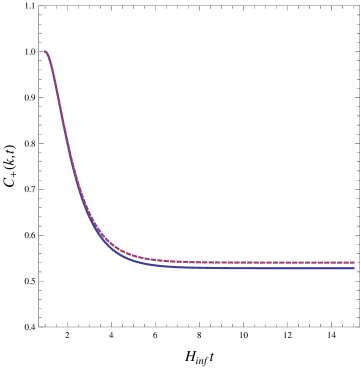
Figure 2: $C_{+}(k,t)$ as a function of $H_{\mathrm{inf}}t$. The legend is the same as in Fig. 1 except $H_{\mathrm{inf}}=1.0\times 10^{13}$GeV and $m=2.44\times 10^{12}$GeV. (the case (A) in Tables 2 and 4).

In Fig. 2, we display the evolution of $C_{+}(k,t)$ during inflation with the solid line for $X(t_{k})\equiv\exp\left(\chi_{k}\right)$ with $\chi_{k}=-0.940$, $H_{\mathrm{inf}}=1.0\times 10^{13}$GeV, $M=1.0\times 10^{-1}M_{\mathrm{P}}=2.43\times 10^{17}\,\mathrm{GeV}$, $m=2.44\times 10^{12}$GeV, $\bar{V}=5.07\times 10^{-11}M_{\mathrm{P}}^{4}$, $Y_{k}=7.70\times 10^{-2}M_{\mathrm{P}}=1.87\times 10^{17}\,\mathrm{GeV}$, and $g_{\mathrm{ps}}=1.0$. This is the case (A) in Tables 2 and 4 presented later. The procedure of the numerical calculation is the same as the one used to derive the results in Fig. 1. The qualitative features of evolution of $C_{+}(k,t)$ is equivalent to those shown in Fig. 1, namely, $C_{+}(k,t)$ becomes a constant around the 10 Hubble expansion time after the first horizon crossing during inflation. Even for different values of $H_{\mathrm{inf}}$, the evolution of $C_{+}(k,t)$ is the same as that in the case described above. Namely, the value of $C_{+}(k,t)$ asymptotically approaches a constant whose value is ${\cal O}(0.1)$.

It follows from the values of the COBE normalization and Planck data that

$$f_{\mathrm{S}}(\xi)\exp\left(4\pi\xi\right)=\frac{25}{144}\times 10^{8}\,,$$ (28)

$$Y_{k}=\pm\frac{M_{\mathrm{P}}}{\sqrt{2}\beta}\left[4\frac{\bar{V}}{M_{\mathrm{P}}^{2}m^{2}\beta^{-2}}+1\pm\sqrt{12\frac{\bar{V}}{M_{\mathrm{P}}^{2}m^{2}\beta^{-2}}+1}\right]^{1/2}\,,$$ (29)

with

$$\beta\equiv\sqrt{\frac{-\left(n_{\mathrm{s}}-1\right)}{8}}\,.$$ (30)

Since $Y$ slowly rolls during inflation, $\xi$ can be considered to be a constant at the inflationary stage. Therefore, we use $\xi\simeq\xi_{k}=\left(g_{\mathrm{ps}}\dot{Y}(t_{k})\right)/\left(2MX(t_{k})H_{\mathrm{inf}}\right)=\left[3Y_{k}/\left(4MX(t_{k})\right)\right]\left\{-1+\sqrt{1+\left[2m/\left(3H_{\mathrm{inf}}\right)\right]^{2}}\right\}\approx\left[Y_{k}/\left(6MX(t_{k})\right)\right]\left(m^{2}/H_{\mathrm{inf}}^{2}\right)$, where the last approximate equality can be met for $m/H_{\mathrm{inf}}\ll 1$. Hence, if the values of $n_{\mathrm{s}}$, $\bar{V}$, and $H_{\mathrm{inf}}$ are given, we can determine those of $m$ and $Y_{k}$. Here, $\bar{V}$ and $M$ can be regarded as free parameters. We take the value of $\bar{V}$ derived from the relation $\bar{V}=3H_{\mathrm{inf}}^{2}M_{\mathrm{P}}^{2}$, which corresponds to the Friedmann equation with $\dot{Y}=0$ at $Y=0$. In this case, in Eq. (29), we find $\bar{V}/\left(M_{\mathrm{P}}^{2}m^{2}\beta^{-2}\right)=3H_{\mathrm{inf}}^{2}/\left(m^{2}\beta^{-2}\right)$. We also get the values of $m$ and $Y_{k}$ with Eqs. (28) and (29). In addition, since the values of $m$ and $Y_{k}$ are real numbers, the values within the square root in Eqs. (28) and (29) have to be larger than or equal to zero. Thus, we obtain the constraint on $\bar{V}$ as $\bar{V}>2\gamma H_{\mathrm{inf}}^{4}$. In what follows, we take the “$+$” sign in front of the right-hand side of $Y_{k}$ in Eq. (29). Consequently, for $m/H_{\mathrm{inf}}\ll 1$, such cases are reasonable during inflation, we have

$$m \approx \sqrt{6}\xi_{k}\frac{M}{M_{\mathrm{P}}}X(t_{k})H_{\mathrm{inf}}\,,$$ (31)

$$Y_{k} \approx \sqrt{6}M_{\mathrm{P}}\frac{H_{\mathrm{inf}}}{m}=\frac{M_{\mathrm{P}}^{2}}{\xi_{k}X(t_{k})M}\,,$$ (32)

where in deriving the last equality in Eq. (32), we have used Eq. (31). As a result, with the value of $\xi_{k}$ from Eq. (28) and substituting it into Eqs. (31) and (32), we obtain the approximate values of $m$ and $Y_{k}$. Indeed, from the lower relation for $2\leq\xi\leq 3$ in Eq. (23), we numerically find that a solution of Eq. (28) is $\xi_{k}=2.5590616$. In the following, we evaluate the value of $m$ with Eq. (31) and that of $Y_{k}$ with Eq. (29).

IV.2 Non-Gaussianity

We suppose that the $\mathrm{U}(1)_{Y}$ gauge field couples to another scalar field, e.g., the Higgs-like field $\varphi$. In this case, the covariant derivative for $\varphi$ is defined by $D_{\mu}\equiv\partial_{\mu}+ig^{\prime}F_{\mu}$, where $g^{\prime}$ is the gauge coupling, and thus the kinetic term of $\varphi$ becomes $\left|D\varphi\right|^{2}$ Meerburg:2012id . Provided that the gauge field obtains its mass through the Higgs mechanism in terms of $\varphi$. The quantum fluctuations of the gauge field mass are produced by the quantum fluctuations of $\varphi$. Eventually, the quantum fluctuations yield in the amount of quanta of the generated gauge field. As a result, the generation of the gauge field leads to the perturbations of number of $e$-folds of inflation $\delta N$. This produces the local type non-Gaussinanity in the anisotropy of the CMB radiation. Non-Gaussianity can be calculated by using the $\delta N$ formalism Sasaki:1995aw ; Starobinsky:1986fxa ; Lyth:2005fi and deriving the curvature perturbations originating from the quantum fluctuations of $\varphi$. When we consider the inflationary model in Ref. Linde:2012bt , by using the COBE Smoot:1992td normalization for the power spectrum of the curvature perturbations $\Delta_{\mathcal{R}}^{2}(k)=2.4\times 10^{-9}$ at $k=k_{*}=0.002\,\mathrm{Mpc}^{-1}$, the local type non-Gaussianity $f_{\mathrm{NL}}^{\mathrm{local}}$ is expressed as Meerburg:2012id

$$f_{\mathrm{NL}}^{\mathrm{local}}\approx 1.0\times 10^{14}\Delta N_{\mathrm{max}}^{3}\frac{g^{\prime}{}^{4}}{\xi^{6}}\frac{m^{2}}{H_{\mathrm{inf}}^{2}}\,.$$ (33)

Here, $\Delta N_{\mathrm{max}}$ is the maximum value of an extra numbers of $e$-folds, and $\xi$ is defined by Eq. (13) with $\dot{Y}$ in Eq. (24).

The reason why in the previous sections, the coupling between $F_{\mu}$ and $\varphi$ through the covariant derivative of $D_{\mu}$ is as follows. Such a coupling might lead to the amplification of the $\mathrm{U}(1)_{Y}$ hypercharge gauge field $F_{\mu}$ during the reheating stage because the conformal invariance of the hypercharge electromagnetic fields is broken through this coupling. However, it has been indicated in Ref. Bassett:2000aw that if the conductivity of the universe is much larger than the Hubble parameter during the reheating stage, such a amplification cannot be realized. Therefore, when we estimate the resultant field strength of the large-scale magnetic fields, it is not necessary to take into consideration this coupling. On the other hand, the physical motivation why we consider the existence of the additional scalar field $\varphi$ and introduce it is the following. It is known that in string theories, the gauge symmetry is broken spontaneously, and the gauge fields obtain their mass. Hence, by introducing the coupling of $F_{\mu}$ to $\varphi$, which evolves to its vacuum expectation value like a Higgs field, we investigate the cosmological consequence of the spontaneous symmetry breaking. In such a case, the number of $e$-folds $N$ during inflation could be changed by the perturbations of $\varphi$, so that the curvature perturbations can be generated through the perturbations of $\varphi$ Meerburg:2012id . As a result, the local-type non-Gaussianity in terms of the curvature perturbations is produced.

Table 2: Local type non-Gaussianity of the curvature perturbations. Legend is the same as in Table 1 with $\Delta N_{\mathrm{max}}=1.0$. The value of $\bar{V}$ is determined by using the relation $\bar{V}=3H_{\mathrm{inf}}^{2}M_{\mathrm{P}}^{2}$ as $\bar{V}=5.07\times 10^{-11}M_{\mathrm{P}}^{4}$ for the case (A) and $\bar{V}=5.07\times 10^{-13}M_{\mathrm{P}}^{4}$ for the case (B). The value of $C_{+}(k,t_{\mathrm{R}})$ is (the case (A), the case (B)) = $(0.528,0.528)$. Moreover, the current field strength of the magnetic fields on $1$Mpc scale $B(1\mathrm{Mpc},t_{0})\hskip 2.84526pt[\mathrm{G}]$ is (the case (A), the case (B)) = $(1.42\times 10^{-56},1.42\times 10^{-56})$.

	$f_{\mathrm{NL}}^{\mathrm{local}}$	$g^{\prime}{}^{2}$	$H_{\mathrm{inf}}\hskip 2.84526pt[\mathrm{GeV}]$	$m\hskip 2.84526pt[\mathrm{GeV}]$	$Y_{k}/M_{\mathrm{P}}$	$B(H_{0}^{-1},t_{0})\hskip 2.84526pt[\mathrm{G}]$
(A) @	$2.70$ @	$1.13\times 10^{-5}$	$1.0\times 10^{13}$	$2.44\times 10^{12}$ @	$7.70\times 10^{-2}$	$7.15\times 10^{-64}$
(B) @	$2.12\times 10^{8}$ @	$1.0\times 10^{-1}$	$1.0\times 10^{12}$	$2.44\times 10^{11}$ @	$7.70\times 10^{-2}$	$7.15\times 10^{-64}$

Table 3: Local type non-Gaussianity of the curvature perturbations. Legend for the case (C) is the same as the case (B) in Table 2 except $M=1.0\times 10^{-2}M_{\mathrm{P}}=2.43\times 10^{16}\,\mathrm{GeV}$. In the case (C), we obtain $C_{+}(k,t_{\mathrm{R}})=0.423$. Furthermore, the current field strength of the magnetic fields on $1$Mpc scale is $B(1\mathrm{Mpc},t_{0})\hskip 2.84526pt[\mathrm{G}]=3.59\times 10^{-57}$.

	$f_{\mathrm{NL}}^{\mathrm{local}}$	$g^{\prime}{}^{2}$	$H_{\mathrm{inf}}\hskip 2.84526pt[\mathrm{GeV}]$	$m\hskip 2.84526pt[\mathrm{GeV}]$	$Y_{k}/M_{\mathrm{P}}$	$\chi_{k}$	$B(H_{0}^{-1},t_{0})\hskip 2.84526pt[\mathrm{G}]$
(C)	$2.12\times 10^{8}$	$1.0\times 10^{-1}$	$1.0\times 10^{12}$	$2.44\times 10^{11}$	$7.70\times 10^{-2}$	$1.36$	$1.81\times 10^{-64}$

In Table 2, we display the numerical results of local non-Gaussianity $f_{\mathrm{NL}}^{\mathrm{local}}$ of the curvature perturbations by taking $\Delta N_{\mathrm{max}}=1.0$, $M=1.0\times 10^{-1}M_{\mathrm{P}}=2.43\times 10^{17}\,\mathrm{GeV}$, $\bar{V}=5.07\times 10^{-11}M_{\mathrm{P}}^{4}$ ($5.07\times 10^{-13}M_{\mathrm{P}}^{4}$) for the case (A) (the case (B)), $g_{\mathrm{ps}}=1.0$, and $k=2\pi/\left(2997.9h^{-1}\right)\,{\mathrm{Mpc}}^{-1}$ with $h=0.673$. Here, we have used the absolute value of $C_{+}(k,t_{\mathrm{R}})$ to estimate the resultant strength of magnetic fields as in Eq. (18). According to the Planck satellite Ade:2013ydc , the constraint on $f_{\mathrm{NL}}^{\mathrm{local}}$ is given by $f_{\mathrm{NL}}^{\mathrm{local}}=2.7\pm 5.8\,(68\%\,\mathrm{CL})$. This has been improved very much in comparison with the Seven-Year WMAP analysis $-10<f_{\mathrm{NL}}^{\mathrm{local}}<74\,(95\%\,\mathrm{CL})$ Komatsu:2010fb . From Table 2, we find that for the case (A), the values of $f_{\mathrm{NL}}^{\mathrm{local}}$ can be compatible with the Planck data, whereas for the case (B), that of $f_{\mathrm{NL}}^{\mathrm{local}}$ is much larger. The upper limit on $f_{\mathrm{NL}}^{\mathrm{local}}$ of less than or equal to ${\cal O}(1)$ makes the space for our model parameters very small. However, there exists a viable room for the parameters such as the case (A) displayed in Table 2. The constraint on $f_{\mathrm{NL}}^{\mathrm{local}}$ can be met by other close values of the parameters.

We also demonstrate the case (C) of Table 3, in which $\Delta N_{\mathrm{max}}$, $\bar{V}$, $g^{\prime}{}^{2}$, $g_{\mathrm{ps}}$, and $k$ are the same as those in the case (B) of Table 2, while the value of $M$ is smaller than that in Table 2. Even though the value of $M$ is larger, the value of $f_{\mathrm{NL}}^{\mathrm{local}}$ is not changed. Since the upper limit of $f_{\mathrm{NL}}^{\mathrm{local}}$ is less than or equal to ${\cal O}(1)$, we see that the case (C) is not consistent with the observations. Thus, for a region of our model parameters, non-Gaussianity for the spectrum of the curvature perturbations can be compatible with the constraint from the Planck result.

We emphasize that the main feature of our model is the presence of term of $X(t_{k})$, which can make the large-scale magnetic field stronger. The contribution of this factor to non-Gaussianity $f_{\mathrm{NL}}^{\mathrm{local}}$ in Eq. (33) is included through $\xi$ in Eq. (13), $m$ in Eq. (31), and $Y_{k}$ in Eq. (32).

IV.3 Tensor-to-scalar ratio

In addition to the scalar modes of the curvature perturbations, the tensor modes, namely, gravitational waves, can be generated. The tensor-to-scalar ratio $r$ is defined by the ratio of amplitude of the tensor modes to that of the scalar modes. In the context of the present scenario, $r$ reads Barnaby:2011vw

$$r=\begin{cases}16\epsilon(t_{k})&\mbox{for $\xi\lesssim 3$\,,}\\ 7.2\epsilon^{2}(t_{k})&\mbox{for $\xi\to\infty$\,,}\end{cases}$$ (34)

$$\epsilon(t_{k})=\frac{2M_{\mathrm{P}}^{2}m^{4}Y_{k}^{2}}{\left(2\bar{V}-m^{2}Y_{k}\right)^{2}}\,,$$ (35)

where $\epsilon(t_{k})=\epsilon(t=t_{k})$ in Eq. (26), and we have used Eqs. (3) and (7).

We show the estimations of the tensor-to-scalar ratio $r$ in Tables 4 and 5. The cases (A) and (B) are the same as those in Table 2, that is, the values of $H_{\mathrm{inf}}$, $M$, $m$, $Y_{k}$, and $\chi_{k}$ are the same. Similarly, the case (C) is equivalent to that in Table 3. We remark that since the values of $H_{\mathrm{inf}}$ and the ratio of $m$ to $H_{\mathrm{inf}}$ in the case (C) are the same as those in the case (B), the value of $r$ in the case (C) is also equal to that in the case (B). The upper limit from the Planck data is estimated as $r<0.11(95\%\,\mathrm{CL})$ Ade:2013uln . It is expected that future/current experiments for the polarization of the CMB radiation such as POLARBEAR POLARBEAR and LiteBIRD LiteBIRD can detect $r<0.01$, and the future plan of LiteBIRD can observe $r<0.001$ LiteBIRD . As a result, when the magnetic fields on the Hubble horizon scale without the back reaction problem are generated at the present time, both the local non-Gaussianity and tensor-to-scalar ratio of the CMB radiation meeting the constraints from the Planck satellite can be produced in a region of the parameters.

In order to check the effect of the dynamics of the $X$ field, we have also investigated a toy model with the dynamical $X$ field, in which the potential of $X=\exp\left(-\lambda\Phi/M_{\mathrm{P}}\right)$ is given by $U(X)=U(\Phi)=\bar{U}\exp\left(-\tilde{\lambda}\Phi/M_{\mathrm{P}}\right)$ with $\lambda$ a dimensionless constant and $\bar{U}$ a constant. As a consequence, we have acquired qualitatively similar results on the current field strength of the large-scale magnetic fields, non-Gaussianity $f_{\mathrm{NL}}^{\mathrm{local}}$ in Eq. (33), and the tensor-to-scalar ratio $r$ in Eq. (34).

Table 4: Tensor-to-scalar ratio of the curvature perturbations for the cases (A) and (B). Legend is the same as Table 2.

	$r$	$H_{\mathrm{inf}}\hskip 2.84526pt[\mathrm{GeV}]$	$m\hskip 2.84526pt[\mathrm{GeV}]$	$Y_{k}/M_{\mathrm{P}}$
(A)	$1.87\times 10^{-5}$	$1.0\times 10^{13}$	$2.44\times 10^{12}$	$7.70\times 10^{-2}$
(B)	$1.87\times 10^{-5}$	$1.0\times 10^{12}$	$2.44\times 10^{11}$	$7.70\times 10^{-2}$

Table 5: Tensor-to-scalar ratio of the curvature perturbations for the case (C). Legend is the same as Table 3.

	$r$	$H_{\mathrm{inf}}\hskip 2.84526pt[\mathrm{GeV}]$	$m\hskip 2.84526pt[\mathrm{GeV}]$	$Y_{k}/M_{\mathrm{P}}$
(C)	$1.87\times 10^{-5}$	$1.0\times 10^{12}$	$2.44\times 10^{11}$	$7.70\times 10^{-2}$

In addition, we mention that the BICEP2 experiment has recently observed the $B$-mode polarization of the CMB radiation with $r=0.20_{-0.05}^{+0.07}\,(68\%\,\mathrm{CL})$ Ade:2014xna . There are discussions on the way of subtracting the foreground data A-A ; MS-KK . Our investigations related to the BICEP2 result on $r$ is described in Appendix A.

In comparison with the past works, the important property of our model is that there exists the term of $X(t_{k})$ leading to the strong magnetic fields. This term contributes to the tensor-to-scalar ratio $r$ in Eq. (34) with $\epsilon(t_{k})$ in Eq. (35) via $m$ in Eq. (31) and $Y_{k}$ in Eq. (32). In our model, in principle, thanks to the factor of $X(t_{k})$, the large-scale magnetic fields with its strong amplitude to account for the observational values only through the adiabatic compression without dynamo mechanism. The reason why we only have small values of the magnetic field strength in Tables I–III is that in this work, we attempt to simultaneously explain three observational quantities, namely, large-scale magnetic fields, non-Gaussianity of the curvature perturbations, and the tensor-to-scalar ratio. This point is the crucial advantage of our model.

V Conclusions

In the present paper, we have explored the generation of large-scale magnetic fields in a toy model of the so-called moduli inflation. In this model, the conformal invariance of the hypercharge electromagnetic fields are broken due to their coupling to both the scalar and pseudoscalar fields appearing in the framework of string theories. We have studied the current strength of the magnetic fields on the Hubble horizon scale, local non-Gaussianity of the curvature perturbations originating from the existence of the massive gauge fields, and the tensor-to-scalar ratio. As a consequence, it has been shown that in addition to the magnetic fields on the Hubble horizon scale, whose current field strength is compatible with the back reaction problem, local non-Gaussianity and the tensor-to-scalar ratio of the power spectrum of the CMB radiation can be generated, the values of which are consistent with the constraints observed by the Planck satellite, i.e., $f_{\mathrm{NL}}^{\mathrm{local}}=\mathcal{O}$(1) and $r<0.11(95\%\,\mathrm{CL})$ Ade:2013uln .

It should be remarked that one of the most important achievement of this work is to derive the explicit values of three cosmological observables such as the large-scale magnetic fields, local non-Gaussianity, and the tensor-to-scalar ratio for the first time.

Appendix A Axion monodromy inflation

The tensor-to-scalar ratio $r$ in moduli inflation is much smaller than the BICEP2 result, although it is still consistent with the Planck data. In this Appendix, we explore axion monodromy inflation and derive the value of $r$ in order to compare it with that in moduli inflation. We explore the following potential KSY-HKSY

$$V(Y)=AY^{q}\,,\quad q=1\,,$$ (36)

with $A$ a constant. In axion monodromy inflation, there is only the pseudoscalar field $Y$, and therefore the scalar field $\Phi$, i.e., the scalar quantity $X=1$ in Eq. (2) does not exist. Hence, the total Lagrangian becomes $\mathcal{L}$ in Eq. (1) with $X=1$ (namely, $\Phi=0$) and $V(Y)$ in Eq. (36) instead of that in Eq. (3). We note that as the other form of the potential, we can consider $V(Y)=\left(1/2\right)m^{2}Y^{2}$, which follows from the limit $Y/f\ll 1$ of the potential $V(Y)=\lambda^{4}\left(1-\cos\left(Y/f\right)\right)$ analyzed in Refs. Barnaby:2010vf ; Barnaby:2011vw .

For the potential $V(Y)$ in Eq. (36), the slow-roll inflation is supposed to be realized, the solution of Eq. (5) is given by

$$Y=\bar{Y}t\,,\quad\bar{Y}=-\frac{A}{3H_{\mathrm{inf}}}\,.$$ (37)

The field equation of $F_{\mu}$ in Eq. (6) becomes

$$\ddot{F_{i}}(t,\mbox{\boldmath$x$})+H\dot{F_{i}}(t,\mbox{\boldmath$x$})-\frac{1}{a^{2}}{\partial}_{j}{\partial}_{j}F_{i}(t,\mbox{\boldmath$x$})+\frac{g_{\mathrm{ps}}}{M}\frac{1}{a}\frac{A}{3H_{\mathrm{inf}}}\epsilon^{ijk}{\partial}_{j}F_{k}(t,\mbox{\boldmath$x$})=0\,,$$ (38)

where we have used Eq. (37). Moreover, with Eq. (37), $\xi$ in Eq. (13) reads

$$\xi=-\frac{1}{6}\frac{g_{\mathrm{ps}}}{M}\frac{A}{H_{\mathrm{inf}}^{2}}\,.$$ (39)

Clearly, this is not a dynamical quantity but a constant.

By using Eqs. (22) with the COBE normalization $\Delta_{\mathcal{R}}^{2}(k)=2.4\times 10^{-9}$ and (25)–(27) with the Planck data $n_{\mathrm{s}}=0.9603$ and assuming that $t\approx H_{\mathrm{inf}}^{-1}$ during inflation, we find $\epsilon=6.62\times 10^{-3}$ and $A=\left[3/\left(4\sqrt{6}\pi\right)\right]\times 10^{5}H_{\mathrm{inf}}^{3}$. This value of $\epsilon$ is realized if $H_{\mathrm{inf}}=6.51\times 10^{15}$GeV. Moreover, it follows from Eq. (39) that if $M=3.55\times 10^{18}$GeV, $g_{\mathrm{ps}}=1.0$, and $H_{\mathrm{inf}}=6.51\times 10^{15}$GeV, we get $|\xi|=2.98$. From Eq. (39), we obtain $r=16\epsilon=0.106$. This is the same order of the BICEP2 result. Thus, in axion monodromy inflation, the tensor-to-scalar ratio compatible with the BICEP2 result can be produced.

Appendix B Issues of the backreaction and the strong coupling

In this Appendix, we explain the issues of the backreaction and the strong coupling. The back reaction problem by the generation of electromagnetic fields during inflation has been found Campanelli:2013mea ; Demozzi:2009fu ; Kanno:2009ei ; Suyama:2012wh ; Fujita:2012rb ; DMR-C (for more recent related works on the relation between the generated gauge fields and inflation, see Maleknejad:2012fw ; Cembranos:2012ng ; Bartolo:2013msa ; Namba:2013kia ; Nurmi:2013gpa ; Fujita:2014sna ). It has been pointed out Demozzi:2009fu that the amplitude of the current magnetic fields on ${\cal O}(1)$ Mpc scale should be less than $10^{-32}$ G. In such a case, the dynamics of inflation is not disturbed by the back reaction originating from the generation of electromagnetic fields. This means that the strength of the magnetic fields on the Hubble horizon scale should be less than $10^{-35}$G, which can be derived by $B(k,t)\propto\left(k/H_{\mathrm{inf}}^{-1}\right)^{0.8}$ Demozzi:2009fu . Throughout this paper, we take parameter sets (for a given coherence scale $\propto k^{-1}$) in which the current magnetic field strength can satisfy this constraint.

In addition, the strong coupling problem that the very strong gauge coupling is necessary to amplify the gauge fields during inflation has been indicated in Ref. Demozzi:2009fu . Recently, as a solution for this problem, the so-called sawtooth model for the coupling between a scalar field and the $\mathrm{U}(1)_{Y}$ fields has been proposed in Ref. Ferreira:2013sqa . In this scenario, the behavior of the scalar field is a sawtooth path. As a result, the magnetic field strength about $10^{-16}$ G on $1$ Mpc scale at the present time can be generated without facing the strong coupling problem as well as the back reaction problem. Furthermore, according to the updated analysis in Ref. Ferreira:2014hma with the recent data from the BICEP2 experiment Ade:2014xna , the magnetic field strength on $1$ Mpc scale should be less than $10^{-30}$G. It is quite interesting to apply our analysis on the generation of large-scale magnetic fields and the estimation of power spectrum, non-Gaussianity and tensor-to-scalar ratio of the curvature perturbations to more realistic moduli inflation models such as the racetrack inflation model.

The strong coupling problem could be solved in the sawtooth scenario Ferreira:2013sqa ; Ferreira:2014hma . Moreover, in Ref. Caprini:2014mja , it has been pointed out that thanks to the inverse cascade mechanism, the constraints obtained in Ref. Demozzi:2009fu can be evaded. Thus, it is important to study whether the sawtooth-like evolution of the dilaton field leading to the large-scale magnetic fields with their sufficient strength can be realized in moduli inflation or not. It may be useful to investigate the racetrack inflation model with positive exponent potential terms, because they induce a quite high potential wall for a large value of the dilaton field AHK-AHKS .

Appendix C Constraints on the strength of cosmic magnetic fields

In this Appendix, we present the upper bounds of the magnetic field strength. The observations of the CMB radiation imply that the upper limit on the magnetic field strength on $1$Mpc scale is $\sim 10^{-9}$G CMB-Limit ; Giovannini:2008df and that on the magnetic field strength on the scale larger than the present Hubble horizon is $4.8\times 10^{-9}\mathrm{G}$ Barrow:1997mj . In Ref. Pogosian:2013dya , by using the data of the polarized radiation imaging and spectroscopy mission (PRISM) Andre:2013afa , it has been indicated that the magnetic fields with $\sim 10^{-9}$G can be detected.

Moreover, there are other methods, such as the 21cm fluctuations of the neutral hydrogen Tashiro:2006uv , the parameter $\sigma_{8}$ for the density perturbation of matter YIKM , the correlation of the curvature perturbations with the magnetic fields Ganc:2014wia , the data of the fifth science (S5) run from the Laser Interferometer Gravitational-wave Observatory (LIGO) Wang:2008vp , the X-ray galaxy cluster survey by Chandra, the Sunyaev-Zel’divich (S-Z) survey TSLS-TS-TTI , and primordial gravitational waves, namely, the tensor modes of the curvature perturbations, generated during inflation Kuroyanagi:2009ez . The upper limits from these observations are compatible with or weaker than those estimated by using the CMB radiation data. Generic investigations on the spectrum of the large-scale magnetic fields from inflation have been executed in Refs. Bamba:2007hm ; Bonvin:2013tba . With the observations of a blazar, the lower bounds on the cosmic magnetic fields in void regions have also been estimated in Ref. Takahashi:2013uoa .

On the other hand, for the magnetic fields on smaller scales, there are the upper bounds from the BBN. The upper limit of the magnetic field strength on the Hubble horizon scale at the BBN epoch $\sim 9.8\times 10^{-5}h^{-1}\mathrm{Mpc}$ with $h=0.673$ Ade:2013lta , is less than $10^{-6}$G BBN .

Incidentally, various issues related to the cosmic magnetic fields have been discussed: Intergalactic magnetic fields Nikiel-Wroczynski:2013zwa , the relation between cosmological magnetic fields and blazars Tashiro:2013bxa , the influence of decay of the cosmic magnetic fields on the CMB radiation Miyamoto:2013oua , and the secondary anisotropies of the CMB radiation originating from stochastic magnetic fields Kunze:2013iwa . Moreover, constraints on the primordial magnetic fields have been proposed from the conversion between the CMB photon and graviton Chen:2013gva , the interaction of the CMB radiation with an axion Tashiro:2013yea in the context of the axiverse Axiverse , the trispectrum of the CMB radiation Trivedi:2013wqa , and the measurement of the Faraday rotation BS-HF .

Appendix D Cosmological implications

In this Appendix, we state cosmological implications obtained from this work. There exists the possibility of baryogenesis coming from the large-scale magnetic fields generated from inflation. These magnetic fields can yield gravitational waves because the space-time is distorted by the existence of the magnetic fields, and eventually the magnetic helicity can be produced Caprini:2003vc . Moreover, the relation between the magnetic helicity and the cosmic chiral asymmetry has been investigated in detail Tashiro:2012mf . If the magnetic helicity exists before the EWPT, baryon numbers can be produced through the effect of the quantum anomaly Joyce:1997uy ; GS-GS . The coupling of the electromagnetic fields to the pseudoscalar field can lead to the magnetic helicity, and thus moduli inflation driven by an axion-like pseudoscalar field can generate not only the large-scale magnetic fields but also the baryon asymmetry of the universe (for trial scenarios, see, e.g., Bamba:2006km ; Bamba:2007hf ). It is meaningful to build a concrete inflationary model, in which both cosmic magnetic fields and baryons can be generated in the framework of fundamental theories such as string theories describing the physics in the early universe. In addition, a leptogenesis scenario due to the existence of the primordial magnetic fields has been proposed in Ref. Long:2013tha . In Ref. Montiel:2014dia , the idea that the component of dark energy may be non-linear electromagnetic fields has been proposed.

We also state the detectability of cosmic magnetic fields. Current and/or future experiments on the polarizations of the CMB radiation, for example, Planck Ade:2013uln ; Ade:2013lta , QUIET QUIET-1 ; Samtleben:2008rb ; Araujo:2012yh , POLARBEAR POLARBEAR , B-Pol B-Pol , and LiteBIRD LiteBIRD can detect the large-scale magnetic fields with the current strength $\sim 4\times 10^{-11}-10^{-10}$G Caprini:2003vc ; Test . For the magnetic fields with the left-handed magnetic helicity, the field strength $\sim 10^{-14}$G on $\sim 10$Mpc scale can be observed Tashiro:2013ita . Further theoretical investigations on the properties of $B$-mode polarization of the CMB radiation has recently been examined in Ref. Giovannini:2014oia . Furthermore, there have been appeared various ideas to detect primordial magnetic fields such as future observations for low-medium redshift Calabrese:2013lga and the bias of magnification of lensing effects Camera:2013fva . Since there are a number of ways of detecting the cosmic magnetic fields, it is possible to examine the physics in both the early- and late-time universes through the detections of the primordial large-scale magnetic fields, especially, in the void structures or the inter-galactic region.

References

- (1) P. P. Kronberg, Rept. Prog. Phys. 57, 325 (1994); D. Grasso and H. R. Rubinstein, Phys. Rept. 348, 163 (2001) [arXiv:astro-ph/0009061]; C. L. Carilli and G. B. Taylor, Ann. Rev. Astron. Astrophys. 40, 319 (2002) [astro-ph/0110655]; L. M. Widrow, Rev. Mod. Phys. 74, 775 (2002) [arXiv:astro-ph/0207240]; M. Giovannini, Int. J. Mod. Phys. D 13, 391 (2004) [arXiv:astro-ph/0312614]; ibid. 14, 363 (2005) [astro-ph/0412601]; Lect. Notes Phys. 737, 863 (2008) [arXiv:astro-ph/0612378]; A. Kandus, K. E. Kunze and C. G. Tsagas, Phys. Rept. 505, 1 (2011) [arXiv:1007.3891 [astro-ph.CO]]; D. G. Yamazaki, T. Kajino, G. J. Mathew and K. Ichiki, ibid. 517, 141 (2012) [arXiv:1204.3669 [astro-ph.CO]]; R. Durrer and A. Neronov, Astron. Astrophys. Rev. 21, 62 (2013) [arXiv:1303.7121 [astro-ph.CO]].
- (2) L. Biermann and A. Schlüter, Phys. Rev. 82, 863 (1951).
- (3) E. S. Weibel, Phys. Rev. Lett. 2, 83 (1959).
- (4) J. M. Quashnock, A. Loeb, and D. N. Spergel, Astrophys. J. 344, L49 (1989); G. Baym, D. Bodeker and L. D. McLerran, Phys. Rev. D 53, 662 (1996) [arXiv:hep-ph/9507429]; D. Boyanovsky, H. J. de Vega and M. Simionato, ibid. 67, 123505 (2003) [arXiv:hep-ph/0211022]; D. Boyanovsky, M. Simionato and H. J. de Vega, ibid. 67, 023502 (2003) [arXiv:hep-ph/0208272]; R. Durrer and C. Caprini, JCAP 0311, 010 (2003) [arXiv:astro-ph/0305059]; T. Kahniashvili, A. G. Tevzadze and B. Ratra, Astrophys. J. 726, 78 (2011) [arXiv:0907.0197 [astro-ph.CO]]; T. Kahniashvili, A. G. Tevzadze, A. Brandenburg and A. Neronov, Phys. Rev. D 87, 083007 (2013) [arXiv:1212.0596 [astro-ph.CO]].
- (5) A. Vilenkin, Phys. Rept. 121, 263 (1985); T. Vachaspati and A. Vilenkin, Phys. Rev. Lett. 67, 1057 (1991); R. H. Brandenberger, A. -C. Davis, A. M. Matheson and M. Trodden, Phys. Lett. B 293, 287 (1992) [hep-ph/9206232]; K. Dimopoulos and A. -C. Davis, Phys. Rev. D 57, 692 (1998) [hep-ph/9705302]; K. Dimopoulos, ibid. 57, 4629 (1998) [hep-ph/9706513]; D. Battefeld, T. Battefeld, D. H. Wesley and M. Wyman, JCAP 0802, 001 (2008) [arXiv:0708.2901 [astro-ph]]; A. -C. Davis and K. Dimopoulos, Phys. Rev. D 72, 043517 (2005) [hep-ph/0505242]; L. V. Zadorozhna, B. I. Hnatyk and Yu. A. Sitenko, UJP 58, 398 (2013) [arXiv:1305.0029 [astro-ph.CO]].
- (6) Z. Berezhiani and A. D. Dolgov, Astropart. Phys. 21, 59 (2004) [arXiv:astro-ph/0305595]; S. Matarrese, S. Mollerach, A. Notari and A. Riotto, Phys. Rev. D 71, 043502 (2005) [arXiv:astro-ph/0410687]; K. Takahashi, K. Ichiki, H. Ohno and H. Hanayama, Phys. Rev. Lett. 95, 121301 (2005) [arXiv:astro-ph/0502283]; K. Ichiki, K. Takahashi, H. Ohno, H. Hanayama and N. Sugiyama, Science 311, 827 (2006); K. Ichiki, K. Takahashi, N. Sugiyama, H. Hanayama and H. Ohno, Mod. Phys. Lett. A 22, 2091 (2007); K. Takahashi, K. Ichiki and N. Sugiyama, Phys. Rev. D 77, 124028 (2008) [arXiv:0710.4620 [astro-ph]]; E. R. Siegel and J. N. Fry, Astrophys. J. 651, 627 (2006) [arXiv:astro-ph/0604526]; T. Kobayashi, R. Maartens, T. Shiromizu and K. Takahashi, Phys. Rev. D 75, 103501 (2007) [arXiv:astro-ph/0701596]; K. E. Kunze, ibid. 77, 023530 (2008) [arXiv:0710.2435 [astro-ph]]; L. Campanelli, P. Cea, G. L. Fogli and L. Tedesco, ibid. 77, 043001 (2008) [arXiv:0710.2993 [astro-ph]]; S. Maeda, S. Kitagawa, T. Kobayashi and T. Shiromizu, Class. Quant. Grav. 26, 135014 (2009) [arXiv:0805.0169 [astro-ph]]; E. Fenu, C. Pitrou and R. Maartens, Mon. Not. Roy. Astron. Soc. 414, 2354 (2011) [arXiv:1012.2958 [astro-ph.CO]]; K. Ichiki, K. Takahashi and N. Sugiyama, Phys. Rev. D 85, 043009 (2012) [arXiv:1112.4705 [astro-ph.CO]]; S. Saga, M. Shiraishi, K. Ichiki and N. Sugiyama, ibid. 87, 104025 (2013) [arXiv:1302.4189 [astro-ph.CO]]; E. Nalson, A. J. Christopherson and K. A. Malik, arXiv:1312.6504 [astro-ph.CO]; P. Berger, A. Kehagias and A. Riotto, arXiv:1402.1044 [astro-ph.CO]; T. Kobayashi, arXiv:1403.5168 [astro-ph.CO]; B. Osano, arXiv:1403.5505 [gr-qc].
- (7) E. N. Parker, Astrophys. J. 163, 255 (1971); Cosmical Magnetic Fields (Clarendon, Oxford, England, 1979); Ya. B. Zel’dovich, A. A. Ruzmaikin, and D. D. Sokoloff, Magnetic Fields in Astrophysics (Gordon and Breach, New York, 1983).
- (8) A. H. Guth, Phys. Rev. D 23, 347 (1981); K. Sato, Mon. Not. Roy. Astron. Soc. 195, 467 (1981); A. A. Starobinsky, Phys. Lett. B 91, 99 (1980).
- (9) M. S. Turner and L. M. Widrow, Phys. Rev. D 37, 2743 (1988).
- (10) L. Campanelli, Phys. Rev. Lett. 111, 061301 (2013) [arXiv:1304.6534 [astro-ph.CO]].
- (11) A. L. Maroto, Phys. Rev. D 64, 083006 (2001) [arXiv:hep-ph/0008288]; C. G. Tsagas, Class. Quant. Grav. 22, 393 (2005) [arXiv:gr-qc/0407080]; C. G. Tsagas and A. Kandus, Phys. Rev. D 71, 123506 (2005) [arXiv:astro-ph/0504089]; J. D. Barrow and C. G. Tsagas, ibid. 77, 107302 (2008) [Erratum-ibid. D 77, 109904 (2008)] [arXiv:0803.0660 [astro-ph]]; Mon. Not. Roy. Astron. Soc. 414, 512 (2011) [arXiv:1101.2390 [astro-ph.CO]]; S. Maeda, S. Mukohyama and T. Shiromizu, Phys. Rev. D 80, 123538 (2009) [arXiv:0909.2149 [astro-ph.CO]]; M. Giovannini, ibid. 88, 063536 (2013) [arXiv:1307.2454 [hep-th]]; A. P. Kouretsis, arXiv:1312.4631 [gr-qc]; F. A. Membiela, arXiv:1312.2162 [astro-ph.CO]; C. G. Tsagas, arXiv:1412.4806 [astro-ph.CO].
- (12) I. Agullo and J. Navarro-Salas, arXiv:1309.3435 [gr-qc]; I. Agullo, J. Navarro-Salas and A. Landete, arXiv:1409.6406 [gr-qc].
- (13) L. Parker, Phys. Rev. Lett. 21, 562 (1968).
- (14) F. D. Mazzitelli and F. M. Spedalieri, Phys. Rev. D 52, 6694 (1995) [astro-ph/9505140]; G. Lambiase and A. R. Prasanna, ibid. 70, 063502 (2004) [gr-qc/0407071]; K. Bamba and S. D. Odintsov, JCAP 0804, 024 (2008) [arXiv:0801.0954 [astro-ph]]; K. Bamba, S. Nojiri and S. D. Odintsov, Phys. Rev. D 77, 123532 (2008) [arXiv:0803.3384 [hep-th]]; K. Bamba and S. Nojiri, arXiv:0811.0150 [hep-th]; L. Campanelli, P. Cea, G. L. Fogli and L. Tedesco, Phys. Rev. D 77, 123002 (2008) [arXiv:0802.2630 [astro-ph]]; G. Lambiase, S. Mohanty and G. Scarpetta, JCAP 0807, 019 (2008); K. E. Kunze, Phys. Rev. D 81, 043526 (2010) [arXiv:0911.1101 [astro-ph.CO]]; J. B. Jimenez and A. L. Maroto, JCAP 1012, 025 (2010) [arXiv:1010.4513 [astro-ph.CO]]; K. E. Kunze, Phys. Rev. D 87, 063505 (2013) [arXiv:1210.6899 [astro-ph.CO]]; K. Bamba, C. -Q. Geng and L. -W. Luo, JCAP 1210, 058 (2012) [arXiv:1208.0665 [astro-ph.CO]]; arXiv:1307.7448 [astro-ph.CO].
- (15) I. T. Drummond and S. J. Hathrell, Phys. Rev. D 22, 343 (1980).
- (16) B. Ratra, Astrophys. J. 391, L1 (1992).
- (17) D. Lemoine and M. Lemoine, Phys. Rev. D 52, 1955 (1995); ibid. 52, 1955 (1995); M. Gasperini, M. Giovannini and G. Veneziano, Phys. Rev. Lett. 75, 3796 (1995) [arXiv:hep-th/9504083]; M. Giovannini, Phys. Rev. D 64, 061301 (2001) [astro-ph/0104290]; J. Martin and J. Yokoyama, JCAP 0801, 025 (2008) [arXiv:0711.4307 [astro-ph]]; K. Bamba and M. Sasaki, ibid. 0702, 030 (2007) [astro-ph/0611701]; K. Bamba, ibid. 0710, 015 (2007) [arXiv:0710.1906 [astro-ph]]; M. Giovannini, Phys. Lett. B 659, 661 (2008) [arXiv:0711.3273 [astro-ph]]; K. Bamba, N. Ohta and S. Tsujikawa, Phys. Rev. D 78, 043524 (2008) [arXiv:0805.3862 [astro-ph]]; K. Bamba, C. Q. Geng and S. H. Ho, JCAP 0811, 013 (2008) [arXiv:0806.1856 [astro-ph]]; M. Giovannini, ibid. 1004, 003 (2010) [arXiv:0911.0896 [astro-ph.CO]]; K. Bamba, C. Q. Geng, S. H. Ho and W. F. Kao, Eur. Phys. J. C 72, 1978 (2012) [arXiv:1108.0151 [astro-ph.CO]]; S. H. Ho, W. F. Kao, K. Bamba and C. Q. Geng, arXiv:1008.0486 [hep-ph]; M. Giovannini, Phys. Rev. D 88, 083533 (2013) [arXiv:1310.1802 [hep-th]]; M. Giovannini, ibid. 89, 063512 (2014) [arXiv:1312.4832 [hep-th]]; D. Kastor and J. Traschen, Class. Quant. Grav. 31, 075023 (2014) [arXiv:1312.4923 [hep-th]]; K. Atmjeet, I. Pahwa, T. R. Seshadri and K. Subramanian, arXiv:1312.5815 [astro-ph.CO].
- (18) K. Bamba and J. Yokoyama, Phys. Rev. D 69, 043507 (2004) [astro-ph/0310824]; 70, 083508 (2004) [hep-ph/0409237].
- (19) W. D. Garretson, G. B. Field and S. M. Carroll, Phys. Rev. D 46, 5346 (1992) [hep-ph/9209238].
- (20) A. D. Dolgov, Phys. Rev. D 48, 2499 (1993) [hep-ph/9301280].
- (21) J. J. Blanco-Pillado, C. P. Burgess, J. M. Cline, C. Escoda, M. Gomez-Reino, R. Kallosh, A. D. Linde and F. Quevedo, JHEP 0411, 063 (2004) [hep-th/0406230].
- (22) S. Kachru, R. Kallosh, A. D. Linde and S. P. Trivedi, Phys. Rev. D 68, 046005 (2003) [hep-th/0301240].
- (23) N. Barnaby, E. Pajer and M. Peloso, Phys. Rev. D 85, 023525 (2012) [arXiv:1110.3327 [astro-ph.CO]].
- (24) N. Barnaby, J. Moxon, R. Namba, M. Peloso, G. Shiu and P. Zhou, Phys. Rev. D 86, 103508 (2012) [arXiv:1206.6117 [astro-ph.CO]].
- (25) R. Z. Ferreira and M. S. Sloth, arXiv:1409.5799 [hep-ph].
- (26) S. L. Cheng, W. Lee and K. W. Ng, arXiv:1409.2656 [astro-ph.CO].
- (27) M. M. Anber and L. Sorbo, JCAP 0610, 018 (2006) [astro-ph/0606534].
- (28) M. M. Anber and L. Sorbo, Phys. Rev. D 81, 043534 (2010) [arXiv:0908.4089 [hep-th]].
- (29) E. Bugaev and P. Klimai, arXiv:1312.7435 [astro-ph.CO].
- (30) P. D. Meerburg and E. Pajer, JCAP 1302, 017 (2013) [arXiv:1203.6076 [astro-ph.CO]].
- (31) E. Pajer and M. Peloso, Class. Quant. Grav. 30, 214002 (2013) [arXiv:1305.3557 [hep-th]].
- (32) N. Barnaby and M. Peloso, Phys. Rev. Lett. 106, 181301 (2011) [arXiv:1011.1500 [hep-ph]].
- (33) N. Barnaby, R. Namba and M. Peloso, JCAP 1104, 009 (2011) [arXiv:1102.4333 [astro-ph.CO]].
- (34) E. Komatsu and D. N. Spergel, Phys. Rev. D 63, 063002 (2001) [astro-ph/0005036].
- (35) T. Tanaka, T. Suyama and S. Yokoyama, @Class. Quant. Grav. 27, 124003 (2010) [arXiv:1003.5057 [astro-ph.CO]].
- (36) A. Linde, S. Mooij and E. Pajer, Phys. Rev. D 87, 103506 (2013) [arXiv:1212.1693 [hep-th]].
- (37) I. Brown and R. Crittenden, Phys. Rev. D 72, 063002 (2005) [astro-ph/0506570].
- (38) P. A. R. Ade et al. [Planck Collaboration], arXiv:1303.5084 [astro-ph.CO].
- (39) P. A. R. Ade et al. [BICEP2 Collaboration], arXiv:1403.3985 [astro-ph.CO].
- (40) M. J. Duff, B. E. W. Nilsson and C. N. Pope, Phys. Rept. 130, 1 (1986); T. Appelquist, A. Chodos and P. G. O. Freund, Modern Kaluza-Klein Theories (Addison-Wesley, Reading, 1987); J. M. Overduin and P. S. Wesson, Phys. Rept. 283, 303 (1997) [gr-qc/9805018]; Y. Fujii and K. Maeda, The Scalar-Tensor Theory of Gravitation (Cambridge University Press, Cambridge, United Kingdom, 2003); C. N. Pope, Lectures on Kaluza-Klein theory (2000), http://people.physics.tamu.edu/pope/ihplec.pdf .
- (41) K. Bamba, Phys. Rev. D 74, 123504 (2006) [hep-ph/0611152].
- (42) K. Bamba, C. Q. Geng and S. H. Ho, Phys. Lett. B 664, 154 (2008) [arXiv:0712.1523 [hep-ph]].
- (43) K. Freese, J. A. Frieman and A. V. Olinto, Phys. Rev. Lett. 65, 3233 (1990); A. R. Liddle, A. Mazumdar and F. E. Schunck, Phys. Rev. D 58, 061301 (1998) [astro-ph/9804177]; E. J. Copeland, A. Mazumdar and N. J. Nunes, ibid. 60, 083506 (1999) [astro-ph/9904309]; A. Mazumdar, S. Panda and A. Perez-Lorenzana, Nucl. Phys. B 614, 101 (2001) [hep-ph/0107058]; J. E. Kim, H. P. Nilles and M. Peloso, JCAP 0501, 005 (2005) [hep-ph/0409138]; S. Dimopoulos, S. Kachru, J. McGreevy and J. G. Wacker, ibid. 0808, 003 (2008) [hep-th/0507205]; R. Easther and L. McAllister, ibid. 0605, 018 (2006) [hep-th/0512102]; L. McAllister, E. Silverstein and A. Westphal, Phys. Rev. D 82, 046003 (2010) [arXiv:0808.0706 [hep-th]]; R. Flauger, L. McAllister, E. Pajer, A. Westphal and G. Xu, JCAP 1006, 009 (2010) [arXiv:0907.2916 [hep-th]]; N. Kaloper and L. Sorbo, Phys. Rev. Lett. 102, 121301 (2009) [arXiv:0811.1989 [hep-th]].
- (44) P. Adshead and M. Wyman, Phys. Rev. Lett. 108, 261302 (2012) [arXiv:1202.2366 [hep-th]]; Phys. Rev. D 86, 043530 (2012) [arXiv:1203.2264 [hep-th]]; E. Martinec, P. Adshead and M. Wyman, JHEP 1302, 027 (2013) [arXiv:1206.2889 [hep-th]].
- (45) N. D. Birrell and P. C. W. Davies, Quantum fields in curved space (Cambridge University Press, New York, 1982); V. F. Mukhanov and S. Winirzki, Introduction to Quantum Effects in Gravity (Cambridge University Press, New York, 2007).
- (46) G. F. Smoot, C. L. Bennett, A. Kogut, E. L. Wright, J. Aymon, N. W. Boggess, E. S. Cheng and G. De Amici et al., Astrophys. J. 396, L1 (1992).
- (47) P. A. R. Ade et al. [Planck Collaboration], arXiv:1303.5082 [astro-ph.CO].
- (48) P. A. R. Ade et al. [Planck Collaboration], arXiv:1303.5076 [astro-ph.CO].
- (49) E. W. Kolb and M. S. Turner, The Early Universe (Addison-Wesley, Redwood City, California, 1990).
- (50) B. A. Bassett, G. Pollifrone, S. Tsujikawa and F. Viniegra, Phys. Rev. D 63, 103515 (2001) [astro-ph/0010628].
- (51) N. Barnaby, Z. Huang, L. Kofman and D. Pogosyan, Phys. Rev. D 80, 043501 (2009) [arXiv:0902.0615 [hep-th]]; N. Barnaby, ibid. 82, 106009 (2010) [arXiv:1006.4615 [astro-ph.CO]].
- (52) G. Hinshaw et al. [WMAP Collaboration], Astrophys. J. Suppl. 208, 19 (2013) [arXiv:1212.5226 [astro-ph.CO]].
- (53) M. Sasaki and E. D. Stewart, Prog. Theor. Phys. 95, 71 (1996) [astro-ph/9507001].
- (54) A. A. Starobinsky, JETP Lett. 42, 152 (1985) [Pisma Zh. Eksp. Teor. Fiz. 42, 124 (1985)].
- (55) D. H. Lyth and Y. Rodriguez, Phys. Rev. Lett. 95, 121302 (2005) [astro-ph/0504045].
- (56) E. Komatsu et al. [WMAP Collaboration], Astrophys. J. Suppl. 192, 18 (2011) [arXiv:1001.4538 [astro-ph.CO]].
- (57) http://mountainpolarbear.blogspot.jp/.
- (58) http://cmbpol.kek.jp/litebird/.
- (59) P. A. R. Ade et al. [Planck Collaboration], arXiv:1405.0871 [astro-ph.GA]; arXiv:1405.0874 [astro-ph.GA]; R. Adam et al. [Planck Collaboration], arXiv:1409.5738 [astro-ph.CO].
- (60) M. J. Mortonson and U. Seljak, arXiv:1405.5857 [astro-ph.CO]; M. Kamionkowski and E. D. Kovetz, arXiv:1408.4125 [astro-ph.CO].
- (61) T. Kobayashi and O. Seto, Phys. Rev. D 89, 103524 (2014) [arXiv:1403.5055 [astro-ph.CO]]; arXiv:1404.3102 [hep-ph].
- (62) J. Joergensen, F. Sannino and O. Svendsen, Phys. Rev. D 90, 043509 (2014) [arXiv:1403.3289 [hep-ph]]; Q. Gao and Y. Gong, Phys. Lett. B 734, 41 (2014) [arXiv:1403.5716 [gr-qc]]; A. Ashoorioon, K. Dimopoulos, M. M. Sheikh-Jabbari and G. Shiu, arXiv:1403.6099 [hep-th]; M. S. Sloth, arXiv:1403.8051 [hep-ph]; C. Cheng and Q. -G. Huang, arXiv:1404.1230 [astro-ph.CO]; C. Cheng, Q. -G. Huang and W. Zhao, arXiv:1404.3467 [astro-ph.CO]; B. Hu, J. -W. Hu, Z. -K. Guo and R. -G. Cai, arXiv:1404.3690 [astro-ph.CO]; Y. Hamada, H. Kawai and K. -y. Oda, arXiv:1404.6141 [hep-ph]; Q. Gao, Y. Gong and T. Li, arXiv:1405.6451 [gr-qc]; L. Barranco, L. Boubekeur and O. Mena, arXiv:1405.7188 [astro-ph.CO]; J. Martin, C. Ringeval, R. Trotta and V. Vennin, arXiv:1405.7272 [astro-ph.CO]; J. Garcia-Bellido, D. Roest, M. Scalisi and I. Zavala, arXiv:1405.7399 [hep-th]; M. Wail Hossain, R. Myrzakulov, M. Sami and E. N. Saridakis, arXiv:1405.7491 [gr-qc]; K. Bamba, S. Nojiri and S. D. Odintsov, Phys. Lett. B 737, 374 (2014) [arXiv:1406.2417 [hep-th]]; T. Inagaki, R. Nakanishi and S. D. Odintsov, arXiv:1408.1270 [gr-qc]; E. Elizalde, S. D. Odintsov, E. O. Pozdeeva and S. Y. Vernov, arXiv:1408.1285 [hep-th]; M. Dine and L. Stephenson-Haskins, arXiv:1408.0046 [hep-ph]; Y. Hamada, H. Kawai, K. y. Oda and S. C. Park, arXiv:1408.4864 [hep-ph].
- (63) T. Kobayashi, O. Seto and Y. Yamaguchi, arXiv:1404.5518 [hep-ph]; T. Higaki, T. Kobayashi, O. Seto and Y. Yamaguchi, arXiv:1405.0775 [hep-ph].
- (64) V. Demozzi, V. Mukhanov and H. Rubinstein, JCAP 0908, 025 (2009) [arXiv:0907.1030 [astro-ph.CO]].
- (65) S. Kanno, J. Soda and M. a. Watanabe, JCAP 0912, 009 (2009) [arXiv:0908.3509 [astro-ph.CO]].
- (66) T. Suyama and J. Yokoyama, Phys. Rev. D 86, 023512 (2012) [arXiv:1204.3976 [astro-ph.CO]].
- (67) T. Fujita and S. Mukohyama, JCAP 1210, 034 (2012) [arXiv:1205.5031 [astro-ph.CO]].
- (68) R. Durrer, G. Marozzi and M. Rinaldi, Phys. Rev. Lett. 111, 229001 (2013) [arXiv:1305.3192 [astro-ph.CO]]; L. Campanelli, ibid. 111, 229002 (2013) [arXiv:1305.7062 [astro-ph.CO]].
- (69) A. Maleknejad, M. M. Sheikh-Jabbari and J. Soda, Phys. Rept. 528, 161 (2013) [arXiv:1212.2921 [hep-th]].
- (70) J. A. R. Cembranos, A. L. Maroto and S. J. Núñez. Jareño, Phys. Rev. D 87, 043523 (2013) [arXiv:1212.3201 [astro-ph.CO]].
- (71) N. Bartolo, S. Matarrese, M. Peloso and A. Ricciardone, JCAP 1308, 022 (2013) [arXiv:1306.4160 [astro-ph.CO]].
- (72) R. Namba, E. Dimastrogiovanni and M. Peloso, JCAP 1311, 045 (2013) [arXiv:1308.1366 [astro-ph.CO]].
- (73) S. Nurmi and M. S. Sloth, arXiv:1312.4946 [astro-ph.CO].
- (74) T. Fujita and S. Yokoyama, JCAP 1403, 013 (2014) [arXiv:1402.0596 [astro-ph.CO]].
- (75) R. J. Z. Ferreira, R. K. Jain and M. S. Sloth, JCAP 1310, 004 (2013) [arXiv:1305.7151 [astro-ph.CO]].
- (76) R. J. Z. Ferreira, R. K. Jain and M. S. Sloth, arXiv:1403.5516 [astro-ph.CO].
- (77) C. Caprini and L. Sorbo, JCAP 1410, 056 (2014) [arXiv:1407.2809 [astro-ph.CO]].
- (78) H. Abe, T. Higaki and T. Kobayashi, Phys. Rev. D 73, 046005 (2006) [hep-th/0511160]; H. Abe, T. Higaki, T. Kobayashi and O. Seto, ibid. 78, 025007 (2008) [arXiv:0804.3229 [hep-th]].
- (79) K. Subramanian and J. D. Barrow, Phys. Rev. Lett. 81, 3575 (1998) [arXiv:astro-ph/9803261]; T. R. Seshadri and K. Subramanian, ibid. 87, 101301 (2001) [arXiv:astro-ph/0012056]; K. Subramanian and J. D. Barrow, Mon. Not. Roy. Astron. Soc. 335, L57 (2002) [arXiv:astro-ph/0205312]; K. Subramanian, T. R. Seshadri and J. D. Barrow, ibid. 344, L31 (2003) [arXiv:astro-ph/0303014]; H. Tashiro, N. Sugiyama and R. Banerjee, Phys. Rev. D 73, 023002 (2006) [arXiv:astro-ph/0509220]; D. G. Yamazaki, K. Ichiki, T. Kajino and G. J. Mathews, ibid. 77, 043005 (2008) [arXiv:0801.2572 [astro-ph]]; T. Kahniashvili, Y. Maravin and A. Kosowsky, ibid. 80, 023009 (2009) [arXiv:0806.1876 [astro-ph]]; D. G. Yamazaki, K. Ichiki, T. Kajino and G. J. Mathews, ibid. 81, 023008 (2010) [arXiv:1001.2012 [astro-ph.CO]]; J. R. Shaw and A. Lewis, ibid. 86, 043510 (2012) [arXiv:1006.4242 [astro-ph.CO]]; P. Trivedi, K. Subramanian and T. R. Seshadri, ibid. 82, 123006 (2010) [arXiv:1009.2724 [astro-ph.CO]]; M. Shiraishi, D. Nitta, S. Yokoyama, K. Ichiki and K. Takahashi, ibid. 82, 121302 (2010) [Erratum-ibid. D 83, 029901 (2011)] [arXiv:1009.3632 [astro-ph.CO]]; D. G. Yamazaki, ibid. 89, 083528 (2014) [arXiv:1404.5310 [astro-ph.CO]].
- (80) M. Giovannini and K. E. Kunze, arXiv:0804.2238 [astro-ph].
- (81) J. D. Barrow, P. G. Ferreira and J. Silk, Phys. Rev. Lett. 78, 3610 (1997) [arXiv:astro-ph/9701063].
- (82) L. Pogosian, Mon. Not. Roy. Astron. Soc. 438, 2508 (2014) [arXiv:1311.2926 [astro-ph.CO]].
- (83) P. Andre et al. [PRISM Collaboration], arXiv:1306.2259 [astro-ph.CO].
- (84) H. Tashiro and N. Sugiyama, Mon. Not. Roy. Astron. Soc. 372, 1060 (2006) [astro-ph/0607169].
- (85) D. G. Yamazaki, K. Ichiki, T. Kajino and G. J. Mathews, Phys. Rev. D 78, 123001 (2008) [arXiv:0811.2221 [astro-ph]]; ibid. 81, 103519 (2010) [arXiv:1005.1638 [astro-ph.CO]].
- (86) J. Ganc and M. S. Sloth, arXiv:1404.5957 [astro-ph.CO].
- (87) S. Wang, Phys. Rev. D 81, 023002 (2010) [arXiv:0810.5620 [astro-ph]].
- (88) H. Tashiro, J. Silk, M. Langer and N. Sugiyama, arXiv:0807.3888 [astro-ph]; H. Tashiro and N. Sugiyama, arXiv:0908.0113 [astro-ph.CO]; H. Tashiro, K. Takahashi and K. Ichiki, arXiv:1010.4407 [astro-ph.CO].
- (89) S. Kuroyanagi, H. Tashiro and N. Sugiyama, Phys. Rev. D 81, 023510 (2010) [arXiv:0909.0907 [astro-ph.CO]].
- (90) K. Bamba, Phys. Rev. D 75, 083516 (2007) [arXiv:astro-ph/0703647].
- (91) C. Bonvin, C. Caprini and R. Durrer, Phys. Rev. D88, 083515 (2013) [arXiv:1308.3348 [astro-ph.CO]].
- (92) K. Takahashi, M. Mori, K. Ichiki, S. Inoue and H. Takami, Astrophys. J. 771, L42 (2013) arXiv:1303.3069 [astro-ph.CO].
- (93) D. Grasso and H. R. Rubinstein, Phys. Lett. B 379, 73 (1996) [arXiv:astro-ph/9602055]; B. Cheng, A. V. Olinto, D. N. Schramm and J. W. Truran, Phys. Rev. D 54, 4714 (1996) [arXiv:astro-ph/9606163].
- (94) B. Nikiel-Wroczyński, M. Soida, M. Urbanik, R. Beck and D. J. Bomans, Mon. Not. Roy. Astron. Soc. 435, 149 (2013) [arXiv:1307.3447 [astro-ph.CO]].
- (95) H. Tashiro and T. Vachaspati, Phys. Rev. D 87, 123527 (2013) [arXiv:1305.0181 [astro-ph.CO]].
- (96) K. Miyamoto, T. Sekiguchi, H. Tashiro and S. Yokoyama, arXiv:1310.3886 [astro-ph.CO].
- (97) K. E. Kunze, arXiv:1312.5630 [astro-ph.CO].
- (98) P. Chen and T. Suyama, Phys. Rev. D 88, 123521 (2013) [arXiv:1309.0537 [astro-ph.CO]].
- (99) H. Tashiro, J. Silk and D. J. E. Marsh, Phys. Rev. D 88, 125024 (2013) [arXiv:1308.0314 [astro-ph.CO]].
- (100) A. Arvanitaki, S. Dimopoulos, S. Dubovsky, N. Kaloper and J. March-Russell, Phys. Rev. D 81, 123530 (2010) [arXiv:0905.4720 [hep-th]]; H. Yoshino and H. Kodama, Prog. Theor. Phys. 128, 153 (2012) [arXiv:1203.5070 [gr-qc]]; arXiv:1312.2326 [gr-qc]; Int. J. Mod. Phys. Conf. Ser. 7, 84 (2012) [arXiv:1108.1365 [hep-th]].
- (101) P. Trivedi, K. Subramanian and T. R. Seshadri, Phys. Rev. D 89, 043523 (2014) [arXiv:1312.5308 [astro-ph.CO]].
- (102) A. Brandenburg and R. Stepanov, Astrophys. J. 786, 91 (2014) [arXiv:1401.4102 [astro-ph.CO]]; C. Horellou and A. Fletcher, arXiv:1401.4152 [astro-ph.CO].
- (103) C. Caprini, R. Durrer and T. Kahniashvili, Phys. Rev. D 69, 063006 (2004) [arXiv:astro-ph/0304556].
- (104) H. Tashiro, T. Vachaspati and A. Vilenkin, Phys. Rev. D 86, 105033 (2012) [arXiv:1206.5549 [astro-ph.CO]].
- (105) M. Joyce and M. E. Shaposhnikov, Phys. Rev. Lett. 79, 1193 (1997) [astro-ph/9703005].
- (106) M. Giovannini and M. E. Shaposhnikov, Phys. Rev. Lett. 80, 22 (1998) [hep-ph/9708303]; Phys. Rev. D 57, 2186 (1998) [hep-ph/9710234].
- (107) A. J. Long, E. Sabancilar and T. Vachaspati, JCAP 1402, 036 (2014) [arXiv:1309.2315 [astro-ph.CO]].
- (108) A. Montiel, N. Breton and V. Salzano, arXiv:1403.6493 [astro-ph.CO].
- (109) See http://quiet.uchicago.edu/index.php.
- (110) D. Samtleben and f. t. Q. Collaboration, Nuovo Cim. 122B, 1353 (2007) [arXiv:0802.2657 [astro-ph]].
- (111) D. Araujo et al. [QUIET Collaboration], Astrophys. J. 760, 145 (2012) [arXiv:1207.5034 [astro-ph.CO]].
- (112) See http://www.b-pol.org/index.php.
- (113) T. Kahniashvili and B. Ratra, Phys. Rev. D 71, 103006 (2005) [arXiv:astro-ph/0503709]; T. Kahniashvili, New Astron. Rev. 50, 1015 (2006) [arXiv:astro-ph/0605440]; J. R. Kristiansen and P. G. Ferreira, Phys. Rev. D 77, 123004 (2008) [arXiv:0803.3210 [astro-ph]].
- (114) H. Tashiro, W. Chen, F. Ferrer and T. Vachaspati, arXiv:1310.4826 [astro-ph.CO].
- (115) M. Giovannini, Phys. Rev. D 89, 061301 (2014) [arXiv:1402.0394 [astro-ph.CO]].
- (116) E. Calabrese, M. Martinelli, S. Pandolfi, V. F. Cardone, C. J. A. P. Martins, S. Spiro and P. E. Vielzeuf, arXiv:1311.5841 [astro-ph.CO].
- (117) S. Camera, C. Fedeli and L. Moscardini, JCAP 1403, 027 (2014) [arXiv:1311.6383 [astro-ph.CO]].