Supplementary Information

1 Supplementary figures

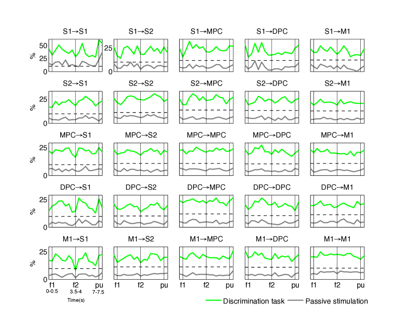
Figure S1: Responsive paths in the first monkey. Percentage of responsive paths in all interarea comparisons during $17$ consecutive task intervals. Arrows in the title indicate the directionality of the modulated paths. Vertical bars outline the intervals $f1$, $f2$ and pu period. Horizontal dashed lines indicate significance level ($\alpha^{\prime}=9.75\%$, where $\alpha^{\prime}=2\alpha(1-\alpha)+\alpha^{2}$ and $\alpha=5\%$). In green, percentages of responsive paths during the discrimination task. In grey, percentages of responsive paths whose correlations were also significant for either the frequency pair ($f1=14$Hz, $f2=22$Hz) or ($f1=30$Hz, $f2=22$Hz) during passive stimulation. Data were obtained in $13$ sessions ($n=13$) from areas S1, primary somatosensory cortex; S2, secondary somatosensory cortex; MPC, medial premotor cortex; DPC, dorsal premotor cortex; M1, primary motor cortex, and were plotted for $17$ consecutive intervals.

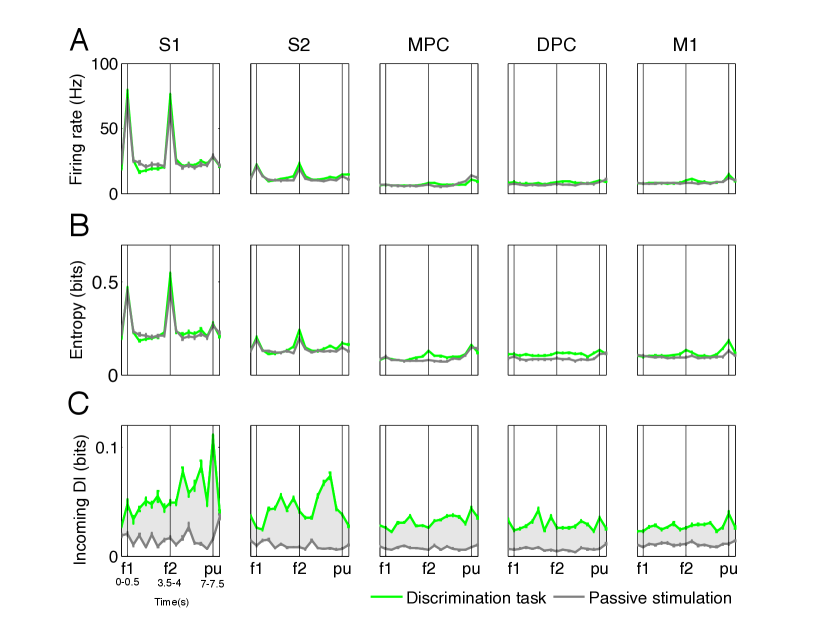
Figure S2: Single-neuron vs. multiple-neuron measures in the first monkey. Comparison between discrimination (green) and passive stimulation tasks (grey) across areas using the average value of distinct measures over the ensemble of neurons with incoming responsive paths. Vertical bars outline the intervals $f1$, $f2$ and pu period. Data were obtained in $13$ sessions ($n=13$) from areas S1, primary somatosensory cortex; S2, secondary somatosensory cortex; MPC, medial premotor cortex; DPC, dorsal premotor cortex; M1, primary motor cortex, and were plotted for $17$ consecutive intervals when $f1=30$Hz and $f2=22$Hz. Error bars ($\pm$ SEM) denote the standard error of each measure. (A) Average firing rate. (B) Average entropy. (C) Average (across the ensemble of neurons) sum of directed information along incoming responsive paths. The shadowed grey area indicates the difference of this measure between both tasks.

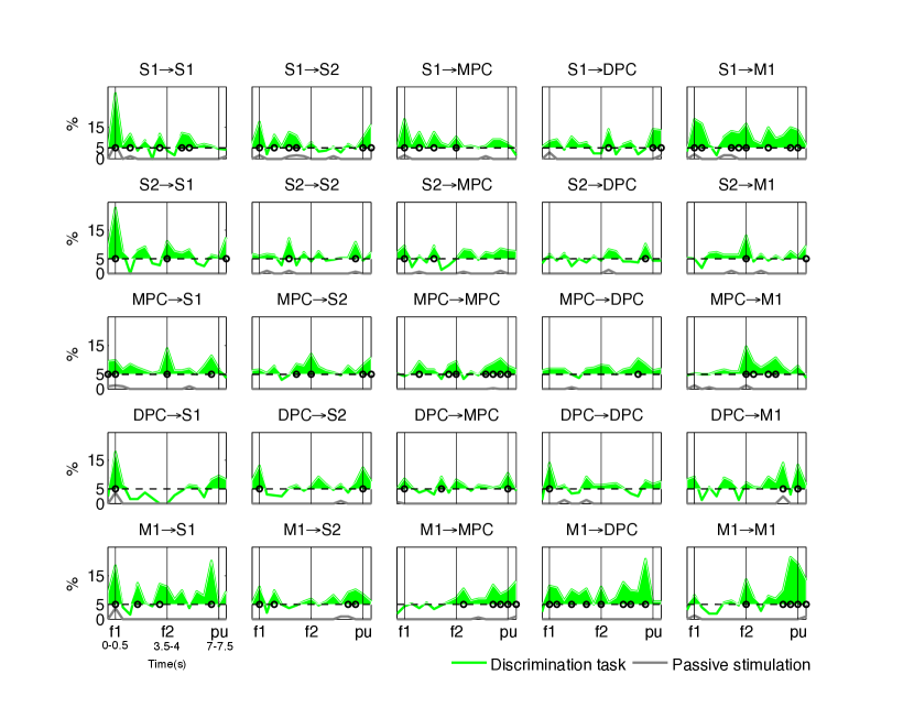
Figure S3: Modulated paths in the first monkey. Percentage of modulated paths over responsive paths in all intra- and interarea comparisons during $17$ consecutive task intervals. In green, percentages during the discrimination task. In grey, percentages during passive stimulation. Arrows in the title indicate the directionality of the modulated paths. Vertical bars outline the intervals $f1$, $f2$ and pu period. Horizontal dashed lines indicate the significance level ($\alpha=5\%$). The shadowed green area indicates the percentages of modulated paths above significance level. Black circles indicate the intervals where the estimated percentage was significantly different (Agresti-Coull confidence interval [1], $\alpha=5\%$) from significance level. Data were obtained in $13$ sessions ($n=13$) from areas S1, primary somatosensory cortex; S2, secondary somatosensory cortex; MPC, medial premotor cortex; DPC, dorsal premotor cortex; M1, primary motor cortex, and were plotted for $17$ consecutive intervals.

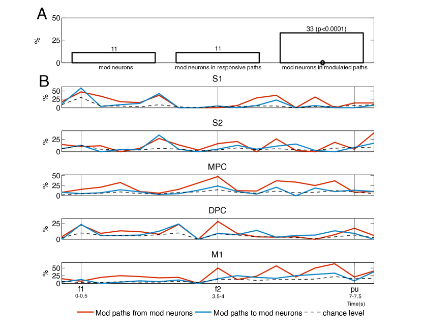
Figure S4: Relationship between modulated neurons and modulated paths in the first monkey. (A) Comparison of the proportion of modulated neurons in all tested neuron pairs (“mod neurons”), responsive (“mod neurons in responsive paths” ) and modulated paths (“mod neurons in modulated paths” ). The black circle highlights that there was a significant correlation between modulated neuron and the existence of an own outgoing or incoming modulated path. (B) Proportion of modulated paths whose starting point neuron or endpoint was a modulated neuron in each recorded area. In red, percentage of outgoing modulated paths from modulated neurons over all modulated outgoing paths from an area (“Mod paths from mod neurons’”). In blue, percentage of incoming modulated paths to modulated neurons over all modulated incoming paths to an area (“Mod paths to mod neurons’”). In dashed black, probability that a modulated neuron was the starting point or endpoint neuron of a randomly selected neuron pair (‘chance level”). Vertical bars outline the intervals $f1$, $f2$ and pu period. Data were obtained in $13$ sessions ($n=13$) from areas S1, primary somatosensory cortex; S2, secondary somatosensory cortex; MPC, medial premotor cortex; DPC, dorsal premotor cortex; M1, primary motor cortex, and were plotted for $17$ consecutive intervals.

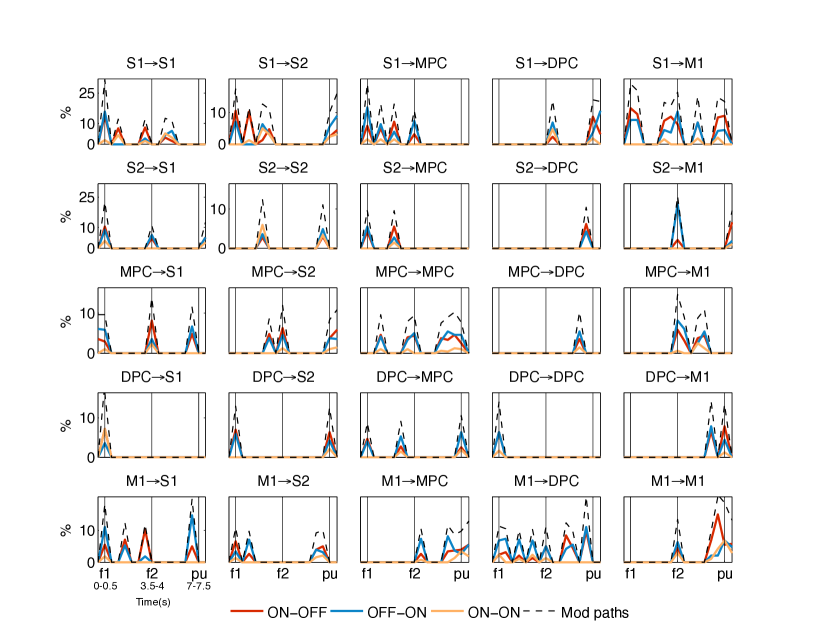
Figure S5: Modulation classes during the discrimination task in the first monkey. Percentage of modulation types in all interarea comparisons and task intervals above significant level ($\alpha=5\%$): percentages of ON-OFF modulations (significant only for $f1<f2$, red), OFF-ON modulations (significant only for $f1>f2$, blue), and ON-ON modulations (significant for both, orange). For reference, the total percentage of modulated paths were plotted in a dashed black line. Arrows in the title indicate the directionality of the modulated paths. Vertical bars outline the intervals $f1$, $f2$ and pu period. Data were obtained in $13$ sessions ($n=13$) from areas S1, primary somatosensory cortex; S2, secondary somatosensory cortex; MPC, medial premotor cortex; DPC, dorsal premotor cortex; M1, primary motor cortex, and were plotted for $17$ consecutive intervals.

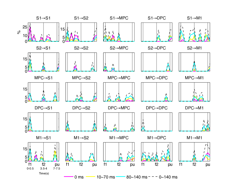
Figure S6: Modulated path delays during the discrimination task in the first monkey. Percentage of modulated path delays in all interarea comparisons and task intervals above significant level ($\alpha=5\%$): percentages of instantaneous correlations ($0$ms, magenta), percentage of modulated paths at delays within $10-70$ms (yellow) and percentages of modulated paths at delays within $80-140$ms (cian). For reference, the total percentage of modulated paths were plotted in a dashed black line. Arrows in the title indicate the directionality of the modulated paths. Vertical bars outline the intervals $f1$, $f2$ and pu period. Data were obtained in $13$ sessions ($n=13$) from areas S1, primary somatosensory cortex; S2, secondary somatosensory cortex; MPC, medial premotor cortex; DPC, dorsal premotor cortex; M1, primary motor cortex, and were plotted for $17$ consecutive intervals.

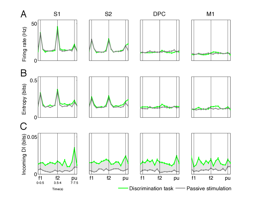
Figure S7: Single-neuron vs. multiple-neuron measures in the second monkey. Comparison between discrimination (green) and passive stimulation tasks (grey) across four areas using the average value of distinct measures over the ensemble of neurons with incoming responsive paths. Data were obtained in $19$ sessions ($n=19$) from areas S1, primary somatosensory cortex; S2, secondary somatosensory cortex; DPC, dorsal premotor cortex; and S1, primary somatosensory cortex; S2, secondary somatosensory cortex; and M1, primary motor cortex and were plotted for $17$ consecutive intervals when $f1=14$Hz and $f2=22$Hz. Vertical bars outline the intervals $f1$, $f2$ and pu period. Error bars ($\pm$ 2SEM) denote the standard error of each measure. (A) Average firing rate. (B) Average entropy. (C) Average (across the ensemble of neurons) sum of directed information along incoming responsive paths. The shadowed grey area indicates the difference of this measure between both tasks.

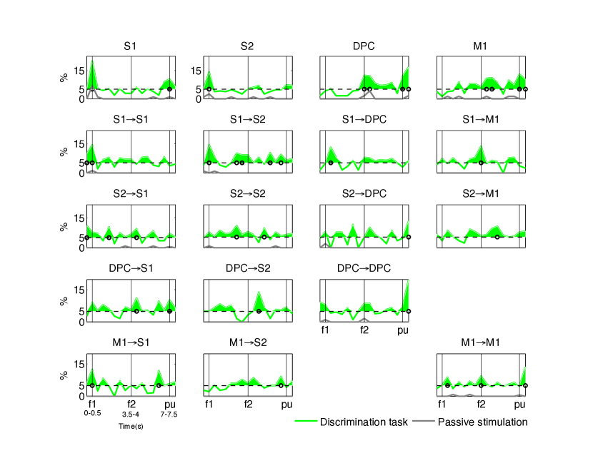
Figure S8: Modulated neurons and paths in the second monkey. In green, percentages during the discrimination task. In grey, percentages during passive stimulation. Arrows in the title indicate the directionality of the modulated paths. Vertical bars outline the intervals $f1$, $f2$ and pu period. Horizontal dashed lines indicate significance level $\alpha=5\%$. The shadowed green area indicates the percentages of modulated paths above significance level. Black circles indicate the intervals where the estimated percentage was significantly different (Agresti-Coull confidence interval [1], $\alpha=5\%$) from significance level. (A) Percentage of modulated neurons over all responsive neurons in each recorded area. (B) Percentage of modulated paths over all responsive paths in $10$ intra- and interarea comparisons. Data were obtained in $19$ sessions ($n=19$) from simultaneous areas S1, primary somatosensory cortex; S2, secondary somatosensory cortex; DPC, dorsal premotor cortex; and S1, primary somatosensory cortex; S2, secondary somatosensory cortex; and M1, primary motor cortex, and were plotted for $17$ consecutive intervals.

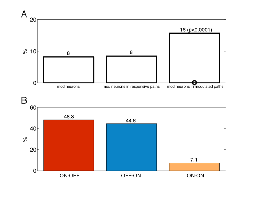
Figure S9: Additional results for the second monkey. (A) Relationship between modulated neurons and modulated paths. Comparison of the proportion of modulated neurons in all tested neuron pairs (“mod neurons”), responsive (“mod neurons in responsive paths” ) and modulated paths (“mod neurons in modulated paths” ). The black circle highlights that there was a significant correlation between modulated neuron and the existence of an own outgoing or incoming modulated path. (B) Modulation classes during the discrimination task. Distribution of modulated paths from intervals above significant level ($\alpha=5\%$) into the classes ON-OFF, OFF-ON and ON-ON.

2 Glossary of terms

• Path: non-linear and (possibly) delayed directional correlation between two neurons. In general, there is no direction defined over a path, but it has an starting point (influencing neuron) and an endpoint neuron (influenced neuron). In this work, correlations are computed using the directed information measure [2].

• Incoming path (to a neuron): a path whose endpoint is the neuron under consideration.

• Outgoing path (from a neuron): a path whose starting point is the neuron under consideration.

• Responsive neuron: a neuron with significant entropy (permutation test, $\alpha=5\%$) for at least one frequency pair.

• Responsive path: a path between responsive neurons for which the value of the directed information (permutation test, $\alpha=5\%$) is significant for at least one frequency pair.

• Modulated neuron: a responsive neuron with significant differences (permutation test, $\alpha=5\%$) in its entropy between the sets of trials $(f1=14,f2=22)$Hz and ($f1=30,f2=22)$Hz.

• Modulated path: a responsive path with significant differences (permutation test, $\alpha=5\%$) in the value of the directed information between the sets of trials $(f1=14,f2=22)$Hz and ($f1=30,f2=22)$Hz.

• ON-ON modulated path: modulated path with significant directed information for both frequency pairs, $(f1=14,f2=22)$Hz and $(f1=30,f2=22)$Hz.

• ON-OFF modulated path: modulated path with significant directed information for the frequency pair $(f1=14,f2=22)$Hz but non-significant for the frequency pair $(f1=30,f2=22)$Hz.

• OFF-ON modulated path: modulated path with significant directed information for the frequency pair $(f1=30,f2=22)$Hz but non-significant for the frequency pair $(f1=14,f2=22)$Hz.

3 Estimation of the directed information

3.1 Notation

Let $X^{T}=(X_{1},\dotsc,X_{T})$ and $Y^{T}=(Y_{1},\dotsc,Y_{T})$ be two random processes that describe the time series $x^{T}=(x_{1},\dotsc,x_{T})$ and $y^{T}=(y_{1},\dotsc,y_{T})$. We shall use $X_{i}$ to denote the $i$-th component of $X^{T}$ and $X^{i}_{j}=(X_{i},\dotsc,X_{j})$, $i<j$, to denote a subset of consecutive components of $X^{T}$. We shall denote the distribution of the joint process $(X^{T},Y^{T})$ as $P_{X^{T}Y^{T}}$ with marginal distributions $P_{X^{T}}$ and $P_{Y^{T}}$.

3.2 Introduction

The majority of methods that estimate information-theoretic quantities between two random processes $X^{T}$ and $Y^{T}$ are based on the computation of the underlying joint probability distribution of a presumed jointly ergodic and stationary process $(\mathcal{X},\mathcal{Y})$. A commonly used estimator in computational neuroscience is the plug-in estimator, which estimates the underlying joint distribution by tracking the frequency of string occurrences in an observed time series [3, 4]. The main drawback of this estimator is the undersampling problem: since all strings are assumed to be equally likely, the estimator requires a sufficiently large number of trials to ensure convergence. Nonetheless, some bias reduction techniques have been proposed to increase the convergence of this estimator [5, 3]. In this work, we follow a Bayesian approach based on the context-tree weighting (CTW) algorithm, [6, 7], which has been proved to outperform the bias and the variance of the plug-in estimator.

In the next sections we provide a general overview of the CTW method. Further implementation details as well as properties of this method can be found in [6]. We start by introducing the concept of tree source model upon which the algorithm is built.

3.3 Tree source model

We consider that sequences of a $M$-ary alphabet (in our case $M$=2) are generated by a tree source of bounded memory $D$, which means that the generation of a symbol $x_{t}$ depends on a suffix of its most recent $D$ symbols $x^{t-1}_{t-D}$. More formally stated, the probability of the generated sequence is defined by the model $({\mathcal{S}},\Theta_{{\mathcal{S}}})$, where ${\mathcal{S}}$ is the suffix set consisting of $M$-ary strings of length no longer than $D$, and

$$\Theta_{{\mathcal{S}}}=(\boldsymbol{\theta}_{s};s\in{\mathcal{S}})$$ (1)

is the parameter space where $\boldsymbol{\theta}_{s}\triangleq(\theta_{0,s},\theta_{1,s},\dotsc,\theta_{M-2,s})$. The suffix set is required to be proper (suffixes in the set are not suffixes of other elements of ${\mathcal{S}}$) and complete (every sequence has a suffix in ${\mathcal{S}}$). Then, we can define a mapping $\beta_{{\mathcal{S}}}(\cdot)$ by which every recent $D$ symbols, $x^{t-1}_{t-D}$, are mapped to a unique suffix $s\in{\mathcal{S}}$. To each suffix, there corresponds a parameter vector $\boldsymbol{\theta}_{s}$ that determines the next symbol probability in the sequence as

$$\Pr\left\{X_{t}=i|x^{t-1}_{t-D},{\mathcal{S}},\Theta_{{\mathcal{S}}}\right\}=\theta_{i,\beta_{{\mathcal{S}}}(x^{t-1}_{t-D})}$$ (2)

for $i=0,\dotsc,M-2$, and

$$\Pr\left\{X_{t}=M-1|x^{t-1}_{t-D},{\mathcal{S}},\Theta_{{\mathcal{S}}}\right\}=1-\prod_{i=0}^{M-2}\theta_{i,\beta_{{\mathcal{S}}}(x^{t-1}_{t-D})}.$$ (3)

The goal of the algorithm is to estimate the probability of any sequence generated by a tree source without knowing the underlying model $({\mathcal{S}},\Theta_{{\mathcal{S}}})$, i.e, without knowing neither the suffix set ${\mathcal{S}}$ nor the parameter space $\Theta$.

Example:

Let $M=2$, $D=2$ and consider the suffix set ${\mathcal{S}}=\{00,10,1\}$. Then, the probability of the sequence $x_{1}^{7}=0110100$, where $x_{1}=0,x_{2}=1,\dots,x_{7}=0$ given the past symbols $10$ can be evaluated as $\Pr\left\{x_{1}^{7}|{\mathcal{S}},\theta_{00},\theta_{10},\theta_{1}\right\}$:

$$\Pr(0110100|10)= P(0|10)\cdot P(1|00)\cdot P(1|01)\cdot P(0|11)\cdot P(1|10)\cdot P(0|01)\cdot P(0|10)$$

$$= (1-\theta_{10})\cdot\,\theta_{00}\,\cdot\,\theta_{1}\cdot(1-\theta_{1})\cdot\,\,\theta_{10}\cdot(1-\theta_{1})\cdot(1-\theta_{10}),$$

where we used the mapping $\beta_{{\mathcal{S}}}(10)=10$, $\beta_{{\mathcal{S}}}(00)=00$, $\beta_{{\mathcal{S}}}(01)=1$ (the sufix 01 is not in the set of suffixes ${\mathcal{S}}$, and we thus map it to the suffix one $\beta_{{\mathcal{S}}}(11)=1$.

3.4 Bayesian approach

The context-tree weighting is a method of approximating the true probability of a $T$-length sequence $x_{1}^{T}$ generated according to the true model $({\mathcal{S}}^{\star},\boldsymbol{\theta}^{\star})$ with the mixture probability

$$\hat{P}(x_{1}^{T})_{=}\sum_{({\mathcal{S}},\Theta_{{\mathcal{S}}})}w({\mathcal{S}},\Theta_{{\mathcal{S}}})P_{{\mathcal{S}},\Theta_{{\mathcal{S}}}}(x_{1}^{T}),$$ (4)

where $w(\cdot)$ is a weighting function over all tree models and $P_{{\mathcal{S}},\Theta_{{\mathcal{S}}}}(x_{1}^{T})$ is the probability of generating the sequence $x_{1}^{T}$ according to the model $({\mathcal{S}},\Theta_{{\mathcal{S}}})$.

To approximate (4), we first make use of the concept of context tree. The context tree is a set of nodes where each node is an $M$-ary string $s$ with length $l(s)$, and where $l(s)$ is upper-bounded by a given memory $D$. Each node $s$ splits into $M$ (child) nodes $0s,1s,\dotsc,(M-1)s$. To each node there corresponds a vector of counts ${\boldsymbol{a}}_{s}=(a_{0,s},a_{1,s},\dotsc,a_{M-1,s})$ of the number of times that a symbol is preceded by the string $s$. For a parent node $s$ and its children $0s,1s,\dotsc,(M-1)s$, the counts must satisfy $a_{i,s}=\sum_{j=0}^{M-1}a_{i,js}$ for every symbol $i=0,\dotsc,M-1$. Then, for every node with string $s$ we estimate the probability that a sequence is generated with the counts ${\boldsymbol{a}}_{s}$. Counts in each node are updated by each new observation $x_{t}$, $t=1,\dotsc,T$.

In general, the probability that a memoryless source with parameter vector $\boldsymbol{\theta}=(\theta_{1},\theta_{2},\dots,\theta_{M})$ generates a given sequence follows a multinomial distribution. By averaging this probability over all possible values of $\theta_{i}$, $i=1,\dots,M$, with a Dirichlet distribution we obtain the Krichevsky-Trofimov (KT) probability estimator. A useful property of this estimator is that it can be sequentially computed as $P^{s}_{e}(0,0,\dotsc,0)=1$ and

$$P^{s}_{e}(a_{0,s},a_{1,s},\dotsc,a_{i-1,s},a_{i,s}+1,a_{i-1,s},\dotsc,a_{M-1,s})=\frac{a_{i,s}+\frac{1}{2}}{a_{0,s}+a_{1,s}+\dotsc+a_{M-1,s}+\frac{M}{2}}.$$ (5)

Finally, we assign a probability to each node, which is the weighted combination of the estimated probability and the weighted probability of its children:

$$P_{w}^{s}=\begin{cases}P_{w}^{s}=\alpha P_{e}^{s}({\boldsymbol{a}}_{s})+(1-\alpha)\prod_{i=1}^{M}P_{w}^{is},\quad&0\leq l(s)<D\\ P_{e}^{s}({\boldsymbol{a}}_{s}),\quad&l(s)=D,\end{cases}$$ (6)

where $\alpha$ is typically chosen to be $\frac{1}{2}$.

3.5 Schematic version of the algorithm for an $M-$ary alphabet

For every $t=1,\dotsc,T$, we use the context $x^{t-1}_{t-D}$ and the value of $x_{t}$. Then, we track nodes from the leaf to the root node along the path determined by $x^{t-1}_{t-D}$.

• Leafs: Identify the leaf $s$ that corresponds to $x^{t-1}_{t-D}$ in the context tree. Then

  1. Counts update
     Based on the value of $x_{t}$, update ${\boldsymbol{a}}_{s}$.

  2. Estimated probability
     Compute $P_{e}^{s}({\boldsymbol{a}}_{s})$ using the Krichevsky-Trofimov estimator, which is defined recursively as $P^{s}_{e}(0,0\dotsc 0)=1$ and for $a_{i,s}\geq 0$, $i=1,\cdots,M-1$,

     $$P_{e}^{s}(a_{0,s},a_{1,s},\dotsc,a_{i-1,s},a_{i,s}+1,a_{i-1,s},\dotsc,a_{M-1,s})=\frac{a_{i,s}+\frac{1}{2}}{a_{0,s}+a_{1,s}+\dotsc+a_{M-1,s}+\frac{M}{2}}.$$

  3. Weighted probability
     For the leaf nodes, $P_{w}^{s}=P_{e}^{s}({\boldsymbol{a}}_{s})$.

• Internal nodes: Using the path determined by the context $x^{t-1}_{t-D}$,
  REPEAT

  1. Parent search
     Identify the parent $s$ of the previously tracked node.

  2. Counts update
     Based on the value of $x_{t}$, update ${\boldsymbol{a}}_{s}$.

  3. Estimated probability
     Compute $P_{e}^{s}({\boldsymbol{a}}_{s})$ using ${\boldsymbol{a}}_{s}$ and the Krichevsky-Trofimov estimator.

  4. Weighted probability
     Compute $P_{w}^{s}$ as

     $$P_{w}^{s}=\alpha P_{e}^{s}(a_{0,s},a_{1,s},\dotsc,a_{M-1,s})+(1-\alpha)\prod_{i=1}^{M}P_{w}^{is},$$

     where $\alpha$ is typically chosen to be $\frac{1}{2}$.
     

  UNTIL the root node is tracked.

• Probability assignment: Let $\lambda$ denote the root node of the context tree. Then, $\hat{P}(x^{t})\equiv P_{w}^{\lambda}(x^{n})$ is the universal probability assignment in the CTW algorithm. As a result, we also obtain the conditional probability $\hat{P}(x_{1}^{t}|x_{1}^{t-1})$ as:

  $$\hat{P}(x_{1}^{t}|x_{1}^{t-1})=\frac{P_{w}^{\lambda}(x_{1}^{t})}{P_{w}^{\lambda}(x^{t-1}_{1})}.$$

Example:

Consider the binary sequence $x^{7}=1011011$ with past symbols $x_{-2}^{0}=101$. We evaluate the context tree for $M=2$ and $D=3$. Suppose that we are at time instance $t=1$ where the context is $101$ (Fig. S10). After observing the sequence up to $t=7$, we obtain counts ${\boldsymbol{a}}_{s}=(a_{0,s},a_{1,s})$ for each context tree node (Fig. S11). From the leafs to the root node ($\lambda$), we recursively compute the weighting probabilities and provide the probability assignment $\hat{P}(x^{7})$ (Fig. S12).

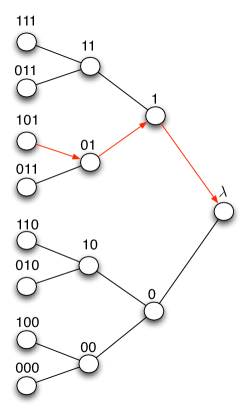
Figure S10: Context tree with the path determined by the context $x^{0}_{-2}=101$ in red.

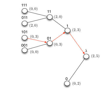
Figure S11: Counts update up to $x_{7}=1$.

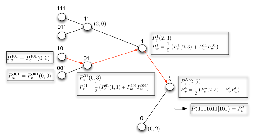
Figure S12: Backward computation of estimated, $P_{e}^{s}({\boldsymbol{a}}_{s})$, weighted probabilities, $P_{w}^{s}$, at $x_{7}=1$, and probability assignment, $\hat{P}(x_{1}^{7})$ .

3.6 Estimator based on the CTW algorithm

The estimator of the directed information that we employ is built upon the CTW algorithm [7]. Then, given a simultaneous observation $(x^{T},y^{T})$, we must assume that it is a realization of a jointly stationary finite-alphabet Markov chain $(\mathcal{X},\mathcal{Y})$ with memory $D$ to ensure estimation consistency. The formula to compute the estimator is the following:

$$\hat{I}(\mathcal{X}\rightarrow\mathcal{Y})\triangleq \frac{1}{T}\sum_{t=1}^{T}\sum_{y_{t}}\hat{P}(Y_{t}=y_{t}\bigl{|}X^{t}_{t-D}=x^{t}_{t-D},Y^{t-1}_{t-D}=y^{t-1}_{t-D})$$

$$\times\log\frac{\hat{P}(Y_{t}=y_{t}\bigl{|}X^{t}_{t-D}=x^{t}_{t-D},Y^{t-1}_{t-D}=y^{t-1}_{t-D})}{\hat{P}(Y_{t}=y_{t}\bigl{|}Y^{t-1}_{t-D}=y^{t-1}_{t-D})},$$ (7)

where the probabilities are estimated using the context-tree weighting method. We next summarize the main steps of this computation:

1. Estimation of the probabilities $\hat{P}(Y_{t}=y_{t}\bigl{|}Y^{t-1}_{t-D}=y^{t-1}_{t-D})$ and $\hat{P}(X_{t}=x_{t},Y_{t}=y_{t}\bigl{|}X^{t-1}_{t-D}=x_{t-D}^{t-1},Y^{t-1}_{t-D}=y_{t-D}^{t-1})$.

2. Computation of the marginal probability

   $$\hat{P}\bigr{(}X_{t}=x_{t}\bigl{|}X^{t-1}_{t-D}=x^{t-1}_{t-D},Y^{t-1}_{t-D}=y^{t-1}_{t-D}\bigl{)}=\sum_{y_{t}}\hat{P}\bigl{(}X_{t}=x_{t},Y_{t}=y_{t}\bigl{|}X^{t-1}_{t-D}=x^{t-1}_{t-D},Y^{t-1}_{t-D}=y^{t-1}_{t-D}\bigr{)}.$$ (8)

3. Application of Bayes theorem using (8):

   $$\hat{P}\bigr{(}Y_{t}=y_{t}\bigl{|}X^{t}_{t-D}=x^{t}_{t-D},Y^{t-1}_{t-D}=y^{t-1}_{t-D}\bigl{)}=\frac{P\bigl{(}X_{t}=x_{t},Y_{t}=y_{t}\bigl{|}X^{t-1}_{t-D}=x^{t-1}_{t-D},Y^{t-1}_{t-D}=y^{t-1}_{t-D}\bigr{)}}{\hat{P}\bigr{(}X_{t}=x_{t}\bigl{|}X^{t-1}_{t-D}=x^{t-1}_{t-D},Y^{t-1}_{t-D}=y^{t-1}_{t-D}\bigl{)}}.$$ (9)

4. Plug-in of (9) and $\hat{P}(Y_{t}=y_{t}\bigl{|}Y^{t-1}_{t-D}=y^{t-1}_{t-D})$ into (7) to obtain $\hat{I}(X^{T}\rightarrow Y^{T})$.

4 Data preprocessing

4.1 Preliminary selection of neurons

We selected $n=13$ recorded sessions from one monkey and $n=19$ recorded sessions from a second monkey. In Tables S1 and S2 we summarize the selected neurons per area and session in the discrimination and passive task.

Session/Area	S1	S2	MPC	DPC	M1
1	5	8	13	4	8
2	6	7	12	9	9
3	5	12	13	9	6
4	5	4	11	8	5
5	1	9	15	3	5
6	7	7	10	5	6
7	2	16	2	6	6
8	2	1	16	2	7
9	1	11	11	4	8
10	0	8	13	9	5
11	5	2	13	4	5
12	4	8	7	6	10
13	4	9	10	6	8
TOTAL	47	102	146	75	88	458

Table S1: Number of neurons per area and session from monkey 1.

Session/Area	S1	S2	DPC	M1
1	4	10	0	5
2	5	8	0	9
3	7	10	0	8
4	4	5	0	12
5	8	13	0	12
6	7	10	0	14
7	6	13	0	15
8	5	7	0	10
9	5	5	3	0
10	8	6	7	0
11	5	11	3	0
12	5	7	11	0
13	5	3	4	0
14	5	6	4	0
15	9	5	7	0
16	4	2	5	0
17	9	8	13	0
18	6	6	12	0
19	8	1	7	0
TOTAL	115	136	76	85	412

Table S2: Number of neurons per area and session from monkey 2.

For each session, we analyzed the following frequency pairs:

$$\Bigl{\{}(f1=14,f2=22)\text{Hz},(f1=30,f2=22)\text{Hz}\Bigr{\}}.$$

We chose the pairs according to two criteria. The first criterion was to maintain the distance between the frequency pairs constant ($|f1-f2|=8$) to neglect effects due to the task difficulty. The second was to keep $f2$ fixed so that we were able to identify neural correlates of the decision after $f2$ stimulation. We only used correct trials in the discrimination task.

4.2 Considerations about the estimator on spike-train data

As introduced before, the consistency of the estimator requires that any pair of simultaneously observed time series is a realization of a jointly stationary irreducible aperiodic Markov process of some bounded order. However, interactions between simultaneously recorded neural responses may occur at different delays depending on the area and the task interval. Furthermore, these interactions may be generated by statistically different processes. To tackle these issues we make the following assumptions:

1. Spike trains can be binarized (i.e., assigning the value $1$ to each bin with at least one spike and the value $0$, otherwise) using a bin size of $2$ms with limited information loss. This assumption is discussed is section 4.2.1.

2. Interactions occur at interneuronal delay values within the range $[0,140]$ms, which is chosen based on the reaction times of each area [9]. This range is binned into the sequence of delays $\delta=[0:5:70]$, i.e., $\delta=0(0\text{ms})$, $5(10\text{ms})$, $10(20\text{ms})$, $\dots,$70$($140$\text{ms})$. We assume that interactions span $4$ms ($D=2$ bins) as it is suggested by a partial analysis of spike-trains entropies discussed in section 4.2.2.

3. We partition the task timeline into $17$ consecutive task intervals of $500$ms, where two intervals match the stimulation periods (Fig. S13). Then, for each task interval and given delay $\delta=[0:5:70]$ bins, any pair of binarized spike trains $(x^{T-\delta},y^{T}_{\delta+1})$, ($T=250$ bins) satisfy the estimator conditions with bounded memory $D=2$ bins.

4. The underlying stationary process of each pair $(x^{T-\delta},y^{T}_{\delta+1})$ is invariant across all trials recorded under the same frequency pair.

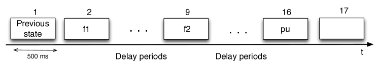
Figure S13: Schematic representation of the division of a trial of $8.5$s into $17$ intervals of $500$ms. The second interval corresponds to the first stimulation, the ninth interval corresponds to the second stimulation and the sixteenth interval corresponds to the probe-up period.

4.2.1 Binarization of spike-train trials

We evaluated the goodness of our bin choice by counting the number of times that more than one spike occurred in one bin and it was neglected. The results illustrated in Table S3 (for a sample of $5$ sessions with trials of $8$s, $n=5$) show that the number of losses was at most $2.7$ spikes per trial.

Area	S1	S2	MPC	DPC	M1
Mean	2.7	0.7	0.1	0.02	0.083

Table S3: Average number of spike losses per trial ($8$s) in a sample of $5$ sessions recorded for the frequency pair $(f1=14,f2=22)$Hz.

4.2.2 Memory and delays

As introduced before, the performance of the CTW algorithm depends on the maximum depth used, $D$, which can be interpreted as the memory of the Markov process underlying an observed time series. Indeed, the computational cost of the algorithm grows exponentially with $D$, and $D$ therefore becomes a critical parameter to set when the number of required estimations is large. To obtain an approximation of neuronal memory we calculated the entropy, $H(Y^{T})$, of all neurons in one session for values of $D$ ranging from $0$ to $9$ during representative task intervals. After inspecting how the average entropy in each area under study stabilized as a function of the spike-train memory, we chose a memory of $D=2$ bins($4$ms) as a good tradeoff between our empirical observation and the dimensionality of the parameter space that we wanted to estimate.

A central question in our study is the time scale at which interactions occur. Results on interarea delays during decision making are scarce in the literature. Instead, the concept of task latency, i.e., the average time before an area is modulated by a task, has been used to approximate the computation of delays during the whole discrimination task [9]. Based on these results, we set the delays within the range $[0,140]$ms.

5 Statistical procedures

Statistical tests were applied in two stages. First, we computed significant values of the directed information across neuron pairs that were simultaneously recorded to find responsive paths. Then, we tested the modulation of significant correlations with respect to the monkey’s decision report to find modulated paths.

5.1 Neuron-pair estimators

We first defined two estimators that were used to correct for multiple testing (one per delay) in each ordered neuron pair. The two estimators were

$$\hat{I}^{(1)}_{\Delta}(X^{T}\rightarrow Y^{T})\triangleq\max_{\delta=[0:5:70]}\hat{I}_{\delta}(\mathcal{X}\rightarrow\mathcal{Y})$$ (10)

$$\hat{I}^{(2)}_{\Delta}(X^{T}\rightarrow Y^{T})\triangleq\sum_{\delta=[0:5:70]}\hat{I}_{\delta}(\mathcal{X}\rightarrow\mathcal{Y}),$$ (11)

where $\hat{I}_{\delta}$ is defined according to (7) for any $\delta>0$:

$$\hat{I}_{\delta}(\mathcal{X}\rightarrow\mathcal{Y})\triangleq \frac{1}{T}\sum_{t=1}^{T}I(Y_{t};X^{t-\delta}|Y^{t-1})$$ (12)

$$= \frac{1}{T}\sum_{t=1}^{T}\sum_{y_{t}}\hat{P}(Y_{t}=y_{t}\bigl{|}X^{t-\delta}_{t-\delta-2}=x^{t-\delta}_{t-\delta-2},Y^{t-1}_{t-2}=y^{t-1}_{t-2})$$

$$\times\log\frac{\hat{P}(Y_{t}=y_{t}\bigl{|}X^{t-\delta}_{t-\delta-2}=x^{t-\delta}_{t-\delta-2},Y^{t-1}_{t-2}=y^{t-1}_{t-2})}{\hat{P}(Y_{t}=y_{t}\bigl{|}Y^{t-1}_{t-2}=y^{t-1}_{t-2})},$$ (13)

and where $\mathcal{X}$ and $\mathcal{Y}$ denote the (marginal) stationary processes of $X^{T}$ and $Y^{T}$. Because of the consistency of the initial estimator (7), it can be checked that (13) is also consistent provided that assumptions 1-4 are satisfied.

5.2 Test on the directed information under fixed stimulation

We considered correct (also named “hit”) trials recorded for the frequency pairs $(f1=14,f2=22)$Hz and $(f1=30,f2=22)$Hz. Based on the assumptions of Section 4.2, we concatenated all trial segments $x^{T-\delta}$ (respectively $y^{T}_{\delta+1}$) that were simultaneously recorded for every delay $\delta=[0:5:70]$. This concatenation was performed preserving the trial chronology of each session. For $\delta\geq 0$, this resulted in a $T^{\prime}$-length time series, where $T^{\prime}=(250-\delta)\times\textrm{number of trials}$ bins (See Fig. S14).

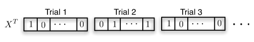
Figure S14: Trial concatenation (for a given neuron, interval, delay and frequency pair).

To assess the statistical significance of the directed information associated with each neuron pair and delay we generated surrogate data by permuting $20$ times the concatenation of the second time series $Y^{T}$ without replacement (See Fig. S15). This procedure destroys all simultaneous dependencies but preserves the statistics of individual concatenated trials. Then, we started by testing all single-neuron entropies to determine which neurons were able to express information about other neurons. Based on this preliminary selection, we tested the (ordered) neuron pairs whose endpoint neuron had a significant entropy. In more detail, for each delay $\delta=0,5\dotsc,70$, we thresholded each original and surrogate data at significance level $\alpha=0.05$ by using a Monte-Carlo permutation test [10], where each value was compared with the distribution obtained by adding the original and the $20$ surrogate estimations. This gave a number of thresholded delays per neuron pair. Then, for every neuron pair, we independently tested the estimators (10) and (11) over all original and surrogate values above the threshold. In particular, for the estimator based on the maximization over delays, $\hat{I}^{(1)}_{\Delta}(X^{T}\rightarrow Y^{T})$, we used again a Monte-Carlo permutation test [10], where this time the original (i.e., non permuted) maximum directed information value over thresholded delays was compared with the tail of a distribution obtained by aggregating maxima surrogate values over corresponding thresholded delays.

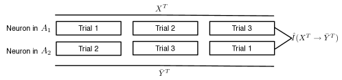
Figure S15: An example of the permutation procedure between two time series $X^{T},\bar{Y}^{T}$.

For the estimator based on the sum of the directed information over delays, $\hat{I}^{(2)}_{\Delta}(X^{T}\rightarrow Y^{T})$, we summed up the directed information across adjacent thresholded delays and used the maximum cluster value as test statistic [11]. Then, we compared the original maximum cluster value with the tail of a distribution obtained by aggregating maxima surrogate values over corresponding clusterized delays. Significant values of each estimator for either the frequency pair $(f1=14,f2=22)$Hz or $(f1=30,f2=22)$Hz defined the responsive paths discussed in the main text.

In order to perform a specific analysis of interneuronal delays, we chose $\hat{I}^{(1)}_{\Delta}(X^{T}\rightarrow Y^{T})$ (10) as our main estimator. Nonetheless, the results using $\hat{I}^{(2)}_{\Delta}(X^{T}\rightarrow Y^{T})$ (11) were similar as Fig. S16 illustrates.

5.3 Test on the modulation of the directed information

To asses the modulation of the directed information with respect to the frequency sign $D=f1-f2$, we performed a permutation test for every ordered pair whose directed information had been shown to be significant for either the frequency pair $(f1=14,f2=22)$Hz or $(f1=30,f2=22)$Hz with the estimators (10)-(11) respectively. For these pre-selected pairs we computed directed information estimates using $5$ trials of each frequency sign. Then, we independently computed the difference between the median and the mean directed information across each set of trials, i.e., $(f1=14,f2=22)$Hz and $(f1=30,f2=22)$Hz, as test statistics. For each statistic we compared the original value (i.e., non permuted) with the tails of a reference distribution obtained by permuting $251$ $\Bigl{(}{10\choose 5}-1\Bigr{)}$ times the $10$ trials without replacement. Significant values were obtained at the two-tailed level $\alpha=0.05$ and defined the modulated paths discussed in the main text. The main results of the paper are based on the difference between the means as test statistic, but no relevant differences were found using the median.

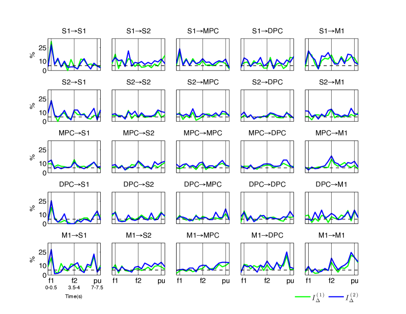
Figure S16: Comparison of the percentage of modulated paths over responsive paths across all intra- and interarea comparisons between the two proposed directed information estimators in the first monkey. One estimator is based on the maximum directed information over delays (in green) and the other based on the sum of the directed information over delays (in blue). The mean difference is used as a modulation test statistic. Arrows in the title indicate the directionality of the modulated paths. Vertical bars outline the intervals $f1$, $f2$ and pu period. Horizontal dashed lines indicate the significance level ($\alpha=5\%$). Data were obtained in $13$ sessions ($n=13$) from areas S1, primary somatosensory cortex; S2, secondary somatosensory cortex; MPC, medial premotor cortex; DPC, dorsal premotor cortex; M1, primary motor cortex, and were plotted for $17$ consecutive intervals.

References

- [1] A. Agresti and B. Coull, “Approximate is better than exact for interval estimation of binomial proportions,” The American Statistician, vol. 52, no. 2, pp. 119–126, 1998.
- [2] J. Massey, “Causality, feedback and directed information,” in Proceedings International Symposium on Information Theory and Applications, 1990, pp. 303–305.
- [3] M. Besserve, B. Schölkopf, N. Logothetis, and S. Panzeri, “Causal relationships between frequency bands of extracellular signals in visual cortex revealed by an information theoretic analysis,” Journal of Computational Neuroscience, vol. 29, no. 3, pp. 547–566, 2010.
- [4] S. Panzeri, N. Brunel, N. Logothetis, and C. Kayser, “Sensory neural codes using multiplexed temporal scales,” Trends Neuroscience, vol. 33, pp. 111–120, 2010.
- [5] S. Panzeri, R. Senatore, M. Montemurro, and R. Petersen, “Correcting for the sampling bias problem in spike train information measures,” Journal of Neurophysiology, vol. 98, pp. 1064–1072, 2007.
- [6] F. Willems, Y. Shtarkov, and T. Tjalkens, “The context-tree weighting method: Basic properties,” IEEE Transactions on Information Theory, vol. 41, no. 3, pp. 653–664, May 1995.
- [7] J. Jiao, H. Permuter, L. Zhao, Y. Kim, and T. Weissman, “Universal estimation of directed information,” IEEE Transactions on Information Theory, vol. 59, no. 10, pp. 6220–6242, 2013.
- [8] Y. Gao, I. Kontoyiannis, and E. Bienenstock, “Estimating the entropy of binary time series: Methodology, some theory and a simulation study,” Entropy, vol. 10, no. 2, pp. 71–99, 2008.
- [9] V. de Lafuente and R. Romo, “Neural correlate of subjective sensory experience gradually builds up across cortical areas,” Proceedings of the National Academy of Sciences, vol. 103, pp. 14 266–14 271, 2006.
- [10] M. Ernst, “Permutation methods: A basis for exact inference,” Statistical Science, vol. 19, no. 4, pp. 676–685, 2004.
- [11] E. Maris and R. Oostenveld, “Nonparametric statistical testing of EEG-and MEG-data,” Journal of neuroscience methods, vol. 164, no. 1, pp. 177–190, 2007.