Individuality and universality in the growth-division laws of single E. coli cells.

Abstract

The mean size of exponentially dividing E. coli cells in different nutrient conditions is known to depend on the mean growth rate only. However, the joint fluctuations relating cell size, doubling time and individual growth rate are only starting to be characterized. Recent studies in bacteria reported a universal trend where the spread in both size and doubling times is a linear function of the population means of these variables. Here, we combine experiments and theory and use scaling concepts to elucidate the constraints posed by the second observation on the division control mechanism and on the joint fluctuations of sizes and doubling times. We found that scaling relations based on the means both collapse size and doubling-time distributions across different conditions, and explain how the shape of their joint fluctuations deviates from the means. Our data on these joint fluctuations highlight the importance of cell individuality: single cells do not follow the dependence observed for the means between size and either growth rate or inverse doubling time. Our calculations show that these results emerge from a broad class of division control mechanisms requiring a certain scaling form of the so-called ”division hazard rate function”, which defines the probability rate of dividing as a function of measurable parameters. This “model free” approach gives a rationale for the universal body-size distributions observed in microbial ecosystems across many microbial species, presumably dividing with multiple mechanisms. Additionally, our experiments show a crossover between fast and slow growth in the relation between individual-cell growth rate and division time, which can be understood in terms of different regimes of genome replication control.

I Introduction

How is the size of a cell at division determined in different environments and conditions? This simple question lies at the foundations of our understanding of cellular growth and proliferation Tzur et al. (2009); Leslie (2011). For some fast-growing bacteria, part of the question was answered between 1958 and 1968, through a series of key studies starting from the seminal work of Schaechter, Maaløe and Kjeldgaard Schaechter et al. (1958). Quoting these authors, size (mass), as well as DNA and RNA content, “could be described as exponential functions of the growth rates afforded by the various media at a given temperature.” Remarkably, these laws for the dependency of mass and intracellular content on population growth rate are fully quantitative, and suggest the possibility of a theory of bacterial physiology, in the way this term is intended by physicists Bremer and Dennis (1996); Scott et al. (2010). Mean growth rate results as the sole “state variable”, not unlike thermodynamic intensive properties such as pressure or concentration. Specifically, the exponent of the Schaechter et al. curve for size has been related to the control of replication initiation Cooper and Helmstetter (1968); Donachie (1968), which is a key regulation step in the cell cycle.

The understanding summarized above, however, solely relates to the average behavior of, e.g., E. coli cells within large colonies. A population can be made of between a handful to billions of cells, each of which will exhibit individual growth and division dynamics, where diversity depends both on fluctuations of the perceived environment and on inherent stochasticity in the decision process underlying cell division. One has then to address how such a heterogeneous collective of growing cells behaves in order to give rise to the Schaechter-Maaløe-Kjeldgaard “growth law”. Thinking of mean growth rate as a “control parameter”, i.e. a scalar variable that the cells may individually measure in their decisions about cell division, one key aspect is whether each cell is individually “aware” of the mean growth conditions to regulate its individual cell division dynamics, or if it simply responds to individual-cell parameters. These two scenarios imply different relationships between the three main observed quantities: cell size, individual growth rate and interdivision time (the two latter quantities cease to be equivalent for single cells), e.g., whether cells dividing at the same rate in different conditions will divide at similar sizes or tend to have similar growth rates. Early experimental efforts to capture this behavior were limited in precision and statistics Koch and Schaechter (1962); Schaechter et al. (1962). Furthermore, such “non-molecular” approaches rapidly came to be considered old-fashioned in favor of the rising paradigm of molecular biology Cooper (1993). Today, the characterization of the fluctuations of cell growth and division across growth conditions remains a largely open question, with potential impact for our general understanding of cell proliferation and its molecular determinants. Additionally, advances in hardware and computational power have made it possible to efficiently collect high-resolution and high-quality data resolved at the single cell level. Recent studies on E. coli Campos et al. (2014); Taheri-Araghi et al. (2014) and B. subtilis Taheri-Araghi et al. (2014) have found a near constancy of the size extension in a single cell cycle (a so-called “adder” mechanism of division control, see also refs. Deforet et al. (2015); Tanouchi et al. (2015)). There is disagreement on whether the same feature is present in C. crescentus Campos et al. (2014); Taheri-Araghi et al. (2014); Iyer-Biswas et al. (2014a); Jun and Taheri-Araghi (2015). One study Taheri-Araghi et al. (2014) reports a universal trend in E. coli where the spread in both size and doubling times is a linear function of the population means of these variables, but also that the joint fluctuations of size and growth rate in a given condition deviates from the mean law followed by the means of these quantities. While the authors show that both behaviors are captured by a suitable “adder” model, they do not address a possible link between them, nor an origin that is more general than the specific division mechanism they consider.

Here, we use a generic scaling theoretical analysis, and a set of high-throughput experiments to fully characterize the joint fluctuations of individual E. coli cell size, growth rate and doubling times in a considerable range of growth conditions, and show their links with the scaling properties. Our experiments confirm the findings of ref. Taheri-Araghi et al. (2014) on the universal scaling and “individual” joint fluctuations of size and growth rate, as well as uncovering novel behavior. Most importantly, the joint fluctuations of growth rate and doubling times also show the same “individualism”, whereby two individuals with the same interdivision time, but coming from two populations with different average growth rate typically do not follow the same behavior in growth rate (and deviate more strongly in faster growth conditions). Our general theoretical approach shows that the diversity in individual cell-size and the scaling are linked by the control of cell division across conditions. Specifically, we calculate the condition under which the control of cell size varies with mean growth rate in such a way that the observed scaling behavior for the distributions of cell size and doubling time is respected, and show that this generally leads to the observed joint fluctuation patterns of doubling times and cell size. Importantly, while our results are compatible with a near-adder division control, we show theoretically that the link between scaling and fluctuations holds beyond this specific mechanism, and cannot be regarded as evidence in favor of a specific mechanism.

In the following we will first introduce the experiment (Fig. 1) and approach the problem from the point of view of the resulting data (Fig. 2 to 5). Subsequently, we will introduce the theoretical approach and show how it unifies the interpretation of the experimental results shown in Fig. 2 (collapse of size and doubling-time distributions) and 5 (joint fluctuations of growth and size). The link between all these results is shown in Fig. 6. Furthermore, Fig. 3 and 4 report measurements on individual growth rate and interdivision times that are not described by the current theories.

II Results

Reliable high-throughput collection of cell division cycles

By using agarose pad microscopy we grew and imaged a large set of colonies in media of varying nutrient quality (Fig. 1). Specifically, we report five physiological conditions from a total of four different nutrient conditions split across two (similar) strains, in the following referred to as P5-ori and MRR (see Methods). A custom-made protocol involving automated imaging and efficient segmentation algorithms (see Methods) gave us wide samples of full cell cycles, typically order ten thousand for each condition, including multiple biological replicates. Since, as we mentioned in the introduction, doubling time and growth rate are not equivalent variables for single cells, it is important to define a consistent terminology. Fig. 1a illustrates the variables measured in our experiment. Since growth in time of single cells is well-described by an exponential Osella et al. (2014); Wang et al. (2010), the growth rate $\alpha$ is defined by an exponential fit. The interdivision time $\tau$ is defined as the time interval between two divisions. The inverse interdivision time defines a “rate” or “frequency” of cell division for a given cell, which can be naturally compared to $\alpha$. Since we also consider a division hazard rate function $h$, which defines how the probability per unit time of dividing changes with internal cell-cycle variables such as instantaneous and initial size, we reserve the wording division rate for $h$, and refer explicitly to inverse interdivision time otherwise. Finally, $V_{0}$ and $V_{f}$ are defined as the estimated spherocylinder volume from the initial and final lengths of the cell and the average width of the cell. Since we monitored cell volume fluctuations across a range of conditions, the changes in cell width made it necessary to estimate cell volume by measuring both width and length of cells (see Methods).

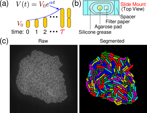
Figure 1: Description of experimental procedure. (a) Schematic of the data collected about each cell. Initial and final volumes $V_{0}$ and $V_{f}$ were estimated from the initial and final lengths of the cell and the width of the cell averaged across its life. The interdivision time $\tau$ was defined as the number of frames between two divisions, multiplied by the time between frames. Since cell growth was well-described by exponential growth Osella et al. (2014); Wang et al. (2010), the growth rate $\alpha$ was defined by fitting the length of the cell to an exponential. (b) Schematic of the agarose pad growth environment. An agarose pad infused with a given growth media was placed on a cover slip, along with a piece of wet filter paper. A dilute bacterial suspension was placed on the agarose pad, sealed with silicone grease, and covered with a second cover slip. The cover slip “sandwich” was placed on the microscope for viewing (see Methods). (c) Example of the raw and processed data. The left panel is a representative “raw” image of a microcolony after several generations of continuously observed growth. The right panel is the result of the segmentation algorithm applied to the raw image (see Methods).

During the analysis, we controlled for a possible dependency of growth parameters on position within the colony, finding that doubling times and growth rates of single cells are not dependent on colony position. However, we found that measured cell sizes on the outer edge of a colony appeared larger, due to an image segmentation bias (Supplementary Fig. S2, see Methods for a discussion). Removing these outer-most cells from the analysis did not affect the results.

Colonies grown on agarose in microscope slides are known to show dependency of growth rates on both time and cell position in the colony. To avoid problems of non-steady growth we designed and optimized our experiment in order to prepare and keep the cells in conditions that were as close as possible to steady growth. Importantly, both the total cell volume and the total number of cells grew exponentially (Supplementary Fig. S1) —consistent with previous reports Wang et al. (2010); Osella et al. (2014); Iyer-Biswas et al. (2014a); Wakamoto et al. (2013); Grant et al. (2014) —and the growth rates of total colony volume and cell number are in good agreement. Further, colony growth rates in agar compared well with bulk growth rates (Supplementary Fig. S3) with the exception of one condition, in which growth on agar was faster than bulk growth. As we shall show, however, these deviations from classic behavior in a single condition do not affect the statistics of cell size fluctuations.

Condition	$\langle V_{0}\rangle$ ($\mu$m3)	$\langle\tau\rangle$ (min)	$\langle\alpha\rangle$ (doublings / hr)
P5ori Glc	1.4	68.2	0.9
P5ori CAA	1.6	38.2	1.5
P5ori RDM	3.4	24.6	2.4
MRR Glc	2.3	31.3	1.8
MRR LB	6.5	20.9	2.9

Table 1: Average values of the main parameters: initial size ($V_{0}$), interdivision time ($\tau$), and growth rate ($\alpha$)

We analyzed 2,000-20,000 cells in each condition (Table 1) that satisfied various technical requirements (completely tracked over their whole cell cycle, did not cross the image border, had a positive growth rate, etc). We also verified that the area growth of microcolonies corresponded very well with the average growth rate of segmented cells, and that the distributions of all measured variables agreed with manually curated data, hence the divisions that the segmentation algorithm failed to capture did not create any relevant bias in the data (Supplementary Fig. S3). The initial size distributions changed gradually with generation, at least in part due to the segmentation problems for cells close to colony edges mentioned above (Supplementary Fig. S5, and Methods section C.4). This change was noticeable, but small relative to the variability present within any one generation. To control for the effect of this time-dependency on results, we analyzed the cells from the range of generations in which the main growth variables are most steady as well as the full data set (Supplementary Fig. S4). From the 2,000-20,000 cell divisions for each condition, about 1000-6000 were in the steadier interval of generations (Supplementary Table S1) Wang et al. (2010). Subsequent analysis reported here refers to these data. Importantly, Supplementary Fig. S6, which reports our main plots on the joint fluctuations of cell size and doubling times for the unrestricted set, shows that the the subsample has the same statistical properties as the whole, and hence shows that our conclusions do not depend on this restriction.

Single-cell size and interdivision times rescale with growth rate.

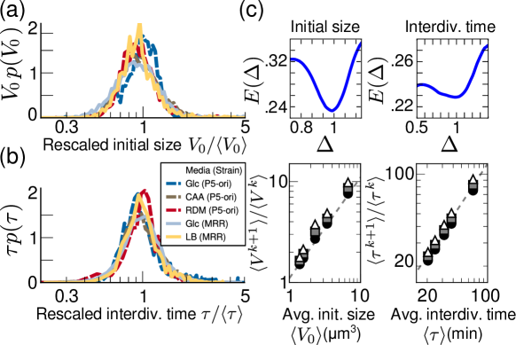
Figure 2: Escherichia coli cell size and interdivision time distributions have a common scaling form across growth conditions. (a) Histograms of initial cell size (from $n>950$ cell cycles each) in different nutrient conditions (represented by different curves) with different mean growth rates, rescaled according to mean initial cell size $V_{0}$ as $p(V_{0})=\frac{1}{V_{0}}F(V_{0}/\langle V_{0}\rangle)$ Giometto et al. (2013). In this and later figures, nutrient conditions are: M9 + Glucose 0.4% (Glc), M9 + casamino acids 0.5% + Glucose 0.4% (CAA), Neidhardt’s rich defined media (RDM) Neidhardt et al. (1974), and LB. See Methods for exact formulations. P5-ori is the shorthand for a BW25113 derivative strain described in the Methods, and MRR is the strain described in Elowitz et al. (2002). (b) same plot as in (a), but for the interdivision time distribution. (c) Top panels: the minimum of the functional $E(\Delta)$ Giometto et al. (2013); Bhattacharjee and Seno (2001) is a measure of the most parsimonious scaling exponent $\Delta$; when evaluated for the distributions of initial size (left) and interdivision time (right), it suggests that the best estimate for the scaling exponent is near to one. (For the definition of $E(\Delta)$, see Methods.) Bottom panels: linear scaling of successive moment ratios for the distributions of initial size (left) and interdivision time (right) confirms the linear scaling behavior. For a quantity $X$ (either initial size or interdivision time), filled circles represent the value of $\langle X^{2}\rangle/\langle X\rangle$ for each condition; grey squares represent $\langle X^{3}\rangle/\langle X^{2}\rangle$; open triangles represent $\langle X^{4}\rangle/\langle X^{3}\rangle$. A dashed line with slope one is shown as a guide to the eye.

We first considered the distributions of three main observables: interdivision time $\tau$, growth rate $\alpha$ (obtained from fitting an exponential to the curve of length vs. time, see Methods), and initial size $V_{0}$. Since the distribution of initial sizes at one generation is defined by the distribution of final sizes in the previous one, in steady growth with binary cell division and equal daughter cell sizes, the distribution of final sizes divided by two has to match the distribution of initial sizes.. We verified that this was the case in our data (Supplementary Fig. S7, since daughters are nearly equalOsella et al. (2014), this condition is applicable to our data).

The distribution of newly-divided cell size is right skewed, and symmetric when plotted on a log scale, resembling a log-normal or a Gamma distribution (Fig. 2a). This is one of the most consistently reported features of E. coli size Henrici (1928); Schaechter et al. (1962); Trueba et al. (1982); Kubitschek and Woldringh (1983); Åkerlund et al. (1995); Wakamoto et al. (2005); Stewart et al. (2005); Wang et al. (2010); Männik et al. (2012); Taheri-Araghi et al. (2014); Campos et al. (2014). We found that the distribution of interdivision time $\tau$ was also positively skewed (Fig. 2b), and resembles a Gaussian on a logarithmic scale. This point has been discussed in the recent literature Iyer-Biswas et al. (2014a); Soifer et al. (2014); Taheri-Araghi et al. (2014); Campos et al. (2014). Both initial size and doubling time distributions across all five growth conditions collapse when rescaled by their means (Fig. 2a,b). This feature was reported early on for E. coli cell sizes Trueba et al. (1982), and very recently also for doubling times Iyer-Biswas et al. (2014a) in Caulobacter crescentus cells growing at different temperatures but constant nutrient conditions.

We tested a finite-size scaling form of these distributions Giometto et al. (2013)

$$p(x)=\frac{1}{x^{\Delta}}F\left(\frac{x}{\langle x\rangle^{1/(2-\Delta)}}\right),$$ (1)

where $p(x)$ is the distribution of a quantity of interest $x$ ($\tau$ or $V_{0}$), $\Delta$ is a scaling exponent, and $F(\xi)$ is the functional shape seen in the distribution of $x$, assumed to be constant for all conditions Giometto et al. (2013); Fisher and Barber (1972). Note that the normalization condition for Eq. (1) requires some constraint on the cutoff of the upper or lower tail of the distribution in order to be compatible with $\Delta\neq 1$ (discussed in the supplementary information of ref. Giometto et al. (2013)). Eq. (1) is a postulate of self-similarity (stating that under a suitable rescaling a set of different curves are in fact the same), classically introduced by Fisher in the context of critical phenomena in statistical physics, justified by behavior of a thermodynamic system near a critical point Cardy (1988). However, in the past decades, it found application very broadly, for example in ecology, including microbial size spectra Giometto et al. (2013); Rinaldo et al. (2002); Banavar et al. (2007, 1999). Using a quantitative method to assess the most parsimonious value for $\Delta$ Bhattacharjee and Seno (2001) based on a cost function $E(\Delta)$ measuring the goodness of the collapse (see Methods), we obtained values very close to unity for this parameter (Fig. 2c). This suggests—as proposed in ref. Giometto et al. (2013)—that these size distributions can be described by a single parameter: their mean. Finally, we found that the scaling prediction that the ratios of successive moments of the size distributions should scale with the mean is verified (Fig. 2c).

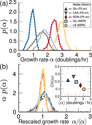
Figure 3: The distribution of single-cell growth rates is symmetric and does not show linear scaling with respect to the mean. (a) Distributions of growth rates $\alpha$ in different conditions. (b) Growth rate distributions rescaled by the means, as in Fig. 2ab, do not collapse. Inset: coefficient of variation of $\alpha$ distributions for each experimental condition, as a function of average growth rate.

In contrast with initial size and doubling time, the distribution of the single-cell growth rates $\alpha$ was more symmetric, and roughly compatible with a Gaussian in all conditions (Fig. 3a), with the two faster growth conditions visibly distinct from the rest when the distributions were rescaled linearly as a test of the finite-size scaling hypothesis (Fig. 3b). Notably, the coefficient of variation (CV) of the growth rate decreases in faster growth conditions, consistent with recent results Kiviet et al. (2014), and hence the distribution does not show a simple linear scaling with the mean across all conditions (Fig. 3b). We also tested scaling with other exponents with the same goodness-of-collapse measurement used for the initial size and interdivision time but the results gave poorer collapse. Indeed, the miminum value of $E(\Delta)$ was noticeably higher than for the other variables (Supplementary Fig. S8). The most parsimonious scaling exponent for the growth rate distribution was $\Delta=0.82$.

Increased deviations from mean-cell behavior at faster growth conditions.

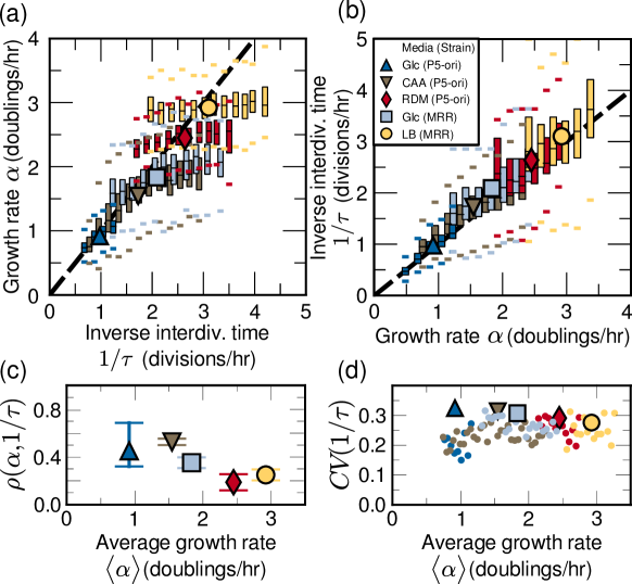
Figure 4: Heterogeneous behaviour of growth rates and interdivision time of single cells. (a) Box plots of growth rate $\alpha$ vs. the inverse interdivision time $1/\tau$, showing that growth rates of cells with similar division frequencies (inverse interdivision times) are similar across slow growth conditions, while this correlation is lost in faster growth conditions. (b) Plot as in (a), but binned instead by growth rate $\alpha$, showing that the mean expected equality of division and doubling rates is restored at the single cell level. Bin width is 0.2 units of $1/\tau$ (in divisions / hr) or $\alpha$ (doublings / hr). Boxes are the inner quartile range and whiskers represent data within 1.5 times the inner quartile range; bins represent at least 50 cells. Large symbols represent population averages. Black dashed lines have a slope of one as a guide to the eye. (c) Pearson correlation coefficient between $\alpha$ and $1/\tau$ across growth conditions. Error bars represent bootstrapped 95% confidence intervals. (d) Coefficient of variation (CV) of $1/\tau$ distribution as a function of growth rate. Large symbols represent the whole population CV; dots represent CV binned by $\alpha$ (bin width 0.05 doublings / hr, each dot represents at least 50 cells). Discrepancy between the large and small dots reveals heterogeneity.

Next, we asked how the growth process of cells influenced cell division. To explore this question, we first analyzed the relation between inverse doubling times $1/\tau$ (i.e., “division frequencies”) and growth rates $\alpha$ of single cells. Fig. 4a shows boxplots of growth rates for cells with different inverse doubling times. As expected —on average— growth rate and inverse doubling time still follow the expected trend $y=x$. This is also confirmed by binning the same data by $\alpha$ (Fig. 4b). Conversely, the behavior of the fluctuations around this mean evidenced by Fig. 4a is different between slow and fast growth conditions. Indeed, in faster growth conditions, cells that divide at a given rate either because of stochasticity or carbon source, can have very different growth rates. More specifically, Fig. 4a shows a transition in behavior at intermediate growth rates between roughly 1.5 and 2 divisions per hour, or equivalently at a crossover time scale of roughly 30 minutes. This crossover is demonstrated by the slope of the plot gradually switching from the straight line $y=x$ (expected for the population means) to a completely flat slope, and by a drop in the Pearson correlation (Fig. 4c) between the two variables, possibly because cells have less time to adapt their division to transient environmental fluctuations. A similar crossover is visible in Fig. 3, although the measured quantity is not the same.

Several additional observations suggest a crossover. The correlation between inverse doubling time $1/\tau$ and initial size $V_{0}$ is stronger when $\langle 1/\tau\rangle$ is less than 2 divisions per hour (Supplementary Fig. S9), and the correlation between $\alpha$ and $V_{0}$ is low except when $\langle\alpha\rangle$ is about 1.5-2 doublings per hour (Supplementary Fig. S9). Finally, for slower growth conditions, the CV of inverse doubling times of a population deviates from the CV of data binned by $\alpha$, indicating that cells with similar individual growth rates have a more homogeneous division frequency in slow-growth conditions, while in faster conditions the variability in their inverse interdivision times increasingly matches the population behavior (Fig. 4d). Taken together, these data clearly indicate that to characterize individual cell behavior one needs to specify both mean population growth rate and a deviation from the mean.

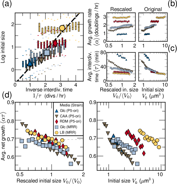
Figure 5: Joint fluctuations of interdivision times and size, and cell division control. (a) Box plots of the logarithm of initial cell size binned by inverse interdivision time. Bins are as in Fig. 4a. Large symbols represent the population averages. The black dashed line represents exponential fit of population averages and is compatible with the Schaechter-Maaløe-Kjeldgaard result. The fluctuations around this mean deviate from the law, more strongly for faster growth conditions. Single-cell growth rate (b), and interdivision time (c) do not show any collapse when plotted as a function of rescaled initial size $V_{0}/\langle V_{0}\rangle$, but average net growth $\alpha\tau$ (commonly used to proxy for size control in cell division Di Talia et al. (2007)) does (d). Each point represents the average value of the corresponding quantity binned by size (bins are constant on log-scale, and each bin is 0.02 units of $\log(V_{0}/\langle V_{0}\rangle)$). Left panels in b,c,d are rescaled versions of the right panels.

Diversity of cell behavior is also evident on the single-cell analogue of the plot from Schaechter, Maaløe, and Kjeldgaard of cell size vs growth rate $\alpha$ or inverse of doubling time $1/\tau$ (Fig. 5a and Supplementary Fig. S10). As previously discussed, inverse doubling time (division frequency) is equivalent to growth rate only when averaged over a population in steady-state growth conditions (i.e., $\langle\alpha\rangle=\log(2)/\langle\tau\rangle$), but the two quantities represent (in principle) independent variables at the single-cell level. Fig. 5a and Supplementary Fig. S10 show that fixing either variable, the deviations from the population behavior become stronger in faster growth conditions; furthermore, the Schaechter-Maaløe-Kjeldgaard “growth law” (stating that for balanced growth, mean cell size increases exponentially when plotted against the mean of the growth rate or the reciprocal of the mean doubling time) does not appear to hold at the single cell level in even the slowest conditions. These findings indicate that also the laws coupling individual cell growth to division (hence to cell size) cannot be extrapolated from the population averages, seemingly in contrast with the universal features of size and doubling time fluctuations. On the other hand, the average sizes of cells growing in different conditions in our data are fully compatible with the expected trend (Fig. 5 and Supplementary Fig. S11).

Fluctuations in cell size and interdivision times are linked to cell division control.

The roles of individual growth rate and doubling time in setting cell division size may be profoundly different. The slope of the plots in Fig. 5a (and Supplementary Fig. S10) may be interpreted as a test for how much a cell that is born larger or smaller than average compensates for this error by modulating its growth or interdivision time. Equivalently, the changes in size control at different growth rates are shown directly by scatter plots of doubling time $\tau$ and single-cell growth rate $\alpha$ versus logarithmic initial size $\log V_{0}$ (Fig. 5b,c). Consistently with previous results Osella et al. (2014), these plots show little correlation between initial size and growth rates (Fig. 5b) and significant anticorrelation between initial size and interdivision time (Fig. 5c), suggesting that the control of cell size should be mostly effected by modulating doubling times rather than growth rate. Additionally, the slopes of these plots show variability across conditions even when rescaled by mean initial size, reinforcing the idea that the extent of this doubling time modulation varies in the different conditions along the Schaechter-Maaløe-Kjeldgaard curve. To test how this is compatible with the observed universal scaling of initial size distributions, we considered another way to quantify size control in cell division, comparing the amount of relative growth within a time interval versus the cell size at the entrance of the interval (Fig. 5d, often referred to as a “size-growth plot”) Osella et al. (2014); Skotheim (2013); Di Talia et al. (2007). The slope of this plot is normally considered a proxy of how much cell division depends on cell size. Fig. 5d shows the average net growth $\langle\alpha\tau\rangle$ vs initial size. These curves show a common slope and, analogously to the size distributions, they collapse when rescaled by the mean initial size in each condition. Note that this is possible only because the correlation of $\alpha$ with $1/\tau$ is nonzero and varies across conditions; one extreme case is LB, where the trend of both $\alpha$ and $1/\tau$ with initial size is very weak, but the trend in Fig. 5d is the same as in other conditions. These results are consistent with a mechanism of cell size control that modulates the division time, such that the scaling is maintained, or, equivalently, operated by a mechanism that contains a single intrinsic length scale Iyer-Biswas et al. (2014a). Our measurements are also consistent with the nearly constant added volume in each cell cycle reported recently for E. coli Jun and Taheri-Araghi (2015) (Supplementary Fig. S13).

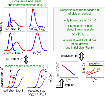
Figure 6: Theoretical analysis showing that division control across different growth conditions is intimately linked to the universal size and doubling-time distributions. Scheme of the theoretical result, which unifies the findings of Fig. 2 and 5. In the cartoons, different colors refer to different conditions. The collapse of initial sizes and doubling times are equivalent to the collapse property of the division rate (Eq. (2)), when plotted as a function of size rescaled by the average initial size, and with $h^{*}$ rescaled by growth rate. The collapse of the size-growth plot in Fig. 5d is a consequence of these properties. The theory predicts that the slope of the fluctuations around the Shaechter-Maaløe-Kjeldgaard law should be the inverse of the mean growth rate.

Theoretical constraints posed by finite-size scaling on division control.

To address the relationship between scaling, cell division control, and individuality in fluctuations observed in our data, we used a theoretical approach (Fig. 6). The framework we employed generally describes cell division through the growth-division process in terms of a division hazard rate function $h^{*}$Osella et al. (2014); Taheri-Araghi et al. (2014). The hazard division rate is defined as the probability per unit time that a cell divides, given the values of the available state variables (e.g., current size, cell-cycle time, etc). This general description allows us to show that the collapse of initial size and doubling time distributions and the fluctuations around the Schaechter-Maaløe-Kjeldgaard law can be explained as a common result of the division control mechanism.

Specifically, we assumed a division hazard rate of the form $h^{*}_{\langle\alpha\rangle}(V,V_{0})$ (for a population with given mean growth rate $\langle\alpha\rangle$), and asked under which conditions this hazard function can generate the observed scaling behavior of the doubling-time and initial-size distributions. This assumption includes as a particular case “adder” models where the control variable is a size difference $V-V_{0}$ Campos et al. (2014); Taheri-Araghi et al. (2014); Soifer et al. (2014) as well as models where elapsed time from cell division is a control variable instead of $V_{0}$, provided the distribution of growth rates is sufficiently peaked Osella et al. (2014). To understand this, note that $h^{*}$ can be a function of all the state variables $(t,V_{0},V,\alpha)$, but under the constraint of exponential growth $V_{f}=V_{0}e^{\alpha\tau}$, different choices of parameters become equivalent. (The full calculation, as well as further details about the formulation of the model, are reported in the Appendix). The essence of the calculation is that the initial size distribution $\rho_{\langle\alpha\rangle}(V_{0})$ can be obtained as a functional of $h^{*}$ by solving the model. One can then impose the finite-size scaling condition on $\rho_{\langle\alpha\rangle}$ and derive the consequences for $h^{*}$. This gives the condition

$$h^{*}_{\langle\alpha\rangle}(V,V_{0})=\langle\alpha\rangle f\left(\frac{V}{\langle V_{0}\rangle_{\langle\alpha\rangle}}\,,\,\frac{V_{0}}{\langle V_{0}\rangle_{\langle\alpha\rangle}}\right)\ .$$ (2)

In other words, our theoretical calculations show that under the condition stated by Eq. (2) (i.e., the scaling form of the division hazard rates from different conditions), the observed scaling behavior for doubling times and initial sizes (Fig. 2) hold, and are equivalent. To test Eq. (2), i.e. the collapse of the division hazard rate $h^{*}_{\langle\alpha\rangle}(V,V_{0})$, with data, we used direct inference from the histograms of dividing cells. The procedure is described in detail in ref. Osella et al. (2014) and in the Appendix, and is based on the fact that, as in a Poisson process, the division hazard rate $h^{*}$ is mathematically related to conditional histograms of undivided cells. Fig. 7ab shows that the condition given in Eq. (2) is verified in our data.

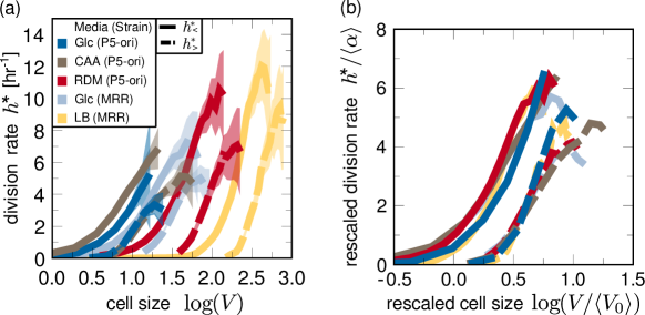
Figure 7: Division hazard rates inferred from data follow the predicted collapse properties. (a) Hazard rate plotted as a function of size, conditional on initial size. $h^{*}_{<}(V)$ (solid lines) is the rate of cell division for cells whose initial size was smaller than the average initial size; $h^{*}_{>}(V)$ (dashed lines) is the rate of cell division for cells whose initial size was larger than the average initial size (the curves would be the same if division depended only on current size Osella et al. (2014); Taheri-Araghi et al. (2014)). (b) the empirical functions $h^{*}_{\langle\alpha\rangle}(V,V_{0})$ follow the collapse property of Eq. (2) (see also Supplementary Fig. S12).

The theory justifies the increased deviations of fluctuations from means in faster growth conditions.

Furthermore, the dependencies of the division hazard rate determine the slope and collapse of the size-growth plot (Appendix and Fig. 5d). Since the size-growth plot is also related to the heterogeneus behavior in the growth of single cells (Fig. 5a and Supplementary Fig. S10), this shows that, while apparently in contrast, the universal behavior of the fluctuations and the deviations of single cells from the Schaechter-Maaløe-Kjeldgaard behavior are in fact two sides of the same coin. This link can be derived directly from Eq. (2), as we report in the Appendix (see also Fig. 6). Here, we support it with the following simple quantitative argument, valid for small fluctuations. Fig. 5d implies that $\alpha\tau\approx\log 2-1/b\log(V_{0}/\langle V_{0}\rangle_{\langle\alpha\rangle})$, where $b\simeq 2$ is a dimensionless constant (the horizontal dashed line in the plot is $\log 2$). However, Fig. 5b shows that most of the correlation with size is contained in $\tau$. One can then suppose that $\alpha\tau\approx\langle\alpha\rangle\tau$. From these two conditions, one gets that

$$(1/\tau)(\log 2-\frac{1}{b}\log(V_{0}/\langle V_{0}\rangle_{\alpha}))\approx\langle\alpha\rangle\ .$$ (3)

Assuming small fluctuations (see also the Appendix, Eq.  (24)), the first term in the left-hand side of this equation can be written as a mean, plus a fluctuation term, $\langle\alpha\rangle+\delta_{1/\tau}$, while the second term is interpreted as a fluctuation of logarithmic size $\delta_{\log V_{0}}$. Assuming small fluctuations, one immediately has that

$$\delta_{\log V_{0}}\approx\frac{\delta_{1/\tau}}{\langle\alpha\rangle}\ .$$ (4)

In other words, the fluctuations in logaritmic cell size around the Schaechter-Maaløe-Kjeldgaard law should become shallower in faster growth conditions, coherently with the observed trend in Fig. 5a.

In conclusion, the joint universality in doubling time and size distributions can be explained by a generic division control mechanism based on a single length scale. Importantly, Eq. (2) shows that other mechanisms, and not only the adder principle, may exhibit both scaling and individuality in the fluctuations. Thus, scaling and individuality are more general and not evidence or simple consequence of near-adder behaviorTaheri-Araghi et al. (2014); Jun and Taheri-Araghi (2015). The Appendix also shows how this result holds using specific examples of division control models Osella et al. (2014). For an adder, Eq. (2) translates into the additional constraint that the division rate $h^{*}_{\langle\alpha\rangle}(V-V_{0})$ should be a function of $\frac{V-V_{0}}{\langle V_{0}\rangle_{\langle\alpha\rangle}}$, which immediately implies the prediction that, in each condition, each moment of order $k$ of the distribution of added size should be proportional to the $k$-th power of $\langle V_{0}\rangle_{\langle\alpha\rangle}$ (since this is the only relevant length scale), while stationarity of the process requires that only their means are equal (as stated in ref. Taheri-Araghi et al. (2014)).

III Discussion and Conclusions

Our study shows that single cells from a given condition with a defined average division rate deviate from the Schaechter-Maaløe-Kjeldgaard “growth law” (which states that mean cell size grows exponentially with mean growth rate), with stronger trend for faster growth conditions. A similar “individuality” in cell behavior relates growth rate to cell division: at slow growth, individual cells appear to adapt their doubling time to match their individual growth rate (thus behaving like a small colony). Conversely, at fast growth the correlation between inverse doubling times and individual growth rates decreases visibly. A crossover time scale around 30 minutes is seen across the data, marking the transition between these two regimes. In analogy with the standard interpretation linking the Schaechter  et al. law with the control of replication initiation Cooper and Helmstetter (1968); Donachie (1968), one can speculate that this characteristic time may be connected to replication time: for example, at fast growth, variability in interdivision times might be more dependent on DNA replication, which becomes increasingly challenging in presence of overlapping rounds, while other determinants of cell division might be more relevant in slow growth. A connection between fluctuations in growth variables and multifork replication is also consistent with the qualitatively different correlations between $\alpha$ and $1/\tau$ observed in our work compared to that recently shown in ref. Iyer-Biswas et al. (2014a), since C. crescentus does not use multifork replication. Iyer-Biswas et al. found that $1/\alpha$ and $\tau$ were well correlated in all growth rates they observed, similarly to our data from slowly growing E. coli, which likely are not undergoing multifork replication.

Our fast-growth results are consistent with findings on cells growing steadily in a microchemostat in rich growth conditions Wang et al. (2010); Osella et al. (2014) and in line with more recent microchemostat results Taheri-Araghi et al. (2014) (Supplementary Fig. S13 and Fig 5a) Finally, we compared our results to previously obtained data in three additional growth media, including poor carbon sources, in order to enhance the range of explored growth rates (Supplementary Fig. S17). These extra experiments were also in line with our main results, showing collapse of size and doubling time distributions, as well as increased deviations from mean behavior at faster growth rates.

We now address the measurements of the distributions of the main variables. The fact that the distribution of cell size is right skewed is one of the most consistently reported features in the E. coli literature Henrici (1928); Schaechter et al. (1962); Trueba et al. (1982); Kubitschek and Woldringh (1983); Åkerlund et al. (1995); Wakamoto et al. (2005); Stewart et al. (2005); Wang et al. (2010); Männik et al. (2012), and it has been derived theoretically using different assumptions about the dynamics (or fluctuations) in the growth process Koch and Schaechter (1962); Hosoda et al. (2011); Amir (2014); Osella et al. (2014); Robert et al. (2014); Giometto et al. (2013). The evidence on the shape of the doubling time distribution has been less consistent, with some studies observing that the distribution is weakly skewed and close to Gaussian Schaechter et al. (1962), and other studies finding positive skew in the distribution Powell (1955); Voorn and Koppes (1998); Ullman et al. (2013); Iyer-Biswas et al. (2014a). The unskewed distribution of the growth rate $\alpha$ has previously been reported for one growth condition Wang et al. (2010); Osella et al. (2014). The $\alpha$ distributions for different mean values $\langle\alpha\rangle$ have been considered in ref. Taheri-Araghi et al. (2014), which appeared while the present work was under review. Interestingly, while this work only tests the collapse with $\Delta=1$, this seems to be good, in some contrast with our agar-derived data. An analytical form of this distribution has been obtained by a recent modeling study Pugatch (2015). The functional form is Log-Fréchet, which appears to fit the published single-cell data better than other forms, and is not collapsible.

The linear finite-size-scaling form of the initial size and doubling times distributions is consistent with recent results in Caulobacter crescentus Iyer-Biswas et al. (2014a) for cells grown at different temperatures. Earlier work had shown such a scaling for size, but had not investigated doubling time Trueba et al. (1982). Our experiments extend the findings in C. crescentus to a phylogenetically distant bacteria with a radically different cell cycle, as well as a complementary perturbation (change of nutrient conditions instead of temperature), showing that the scaling properties of these distributions are unvaried for cells grown at the same temperature in different media. Interestingly, while the linear scaling suggests that the mean behavior (the relative time/length scale) fully sets the shape of the size distribution, the naive expectation would be that the fluctuations around the mean size would also behave equally in different conditions. It is then interesting to ask how these differing properties relate to the shape of the size and doubling-time distributions.

An important standing question is what sets this markedly universal scaling for both size and doubling times. Iyer-Biswas and coworkers Iyer-Biswas et al. (2014a, b) employ an autocatalytic model for growth fluctuations to predict that, within a cell cycle, cell sizes should not follow a multiplicative random walk, but a multiplicative process where the noise scales as the square root of size. Under these conditions, the growth dynamics preserve the scaling of the size distribution, and provided that binary division does not affect this property, scaling should be observed. This reasoning is robust and consistent with data Iyer-Biswas et al. (2014a). However, being focused mostly on growth it does not fully address the possible role of cell division in setting the shape of the distribution.

In our case, we are able to show theoretically that in such models, finite-size scaling of the size and interdivision time distributions is directly related to the collapse of the division hazard rate functions of different conditions, Eq. (2). Since this would not necessarily be the case if the scaling were purely determined by the cell growth process, we are led to surmise that both growth and cell division contribute to the observed size and doubling-time fluctuations. Considering the data, two different measurements of cell division control—the size-growth plot between net growth and initial size (Fig. 5d) and our direct estimate of the division hazard rate as a function of cell size— show rescaling collapse, suggesting that cell division control across conditions contains the same universal scale observed in the size distributions. Hence, since the size-growth plot is also directly related to the fluctuations around the Schaechter-Maaløe-Kjeldgaard curve (Fig. 5a), the outcome of this analysis suggests that both the observed finite-size scaling and the heterogeneity in single-cell behavior across conditions may have a common explanation through cell division control.

It is important to frame this result in the current debate regarding the specific mechanism for the division control. Importantly, our theoretical result is achieved through a “model free” approach, i.e., a generic argument that can apply to a wide range of division mechanisms. Recent works Campos et al. (2014); Taheri-Araghi et al. (2014); Soifer et al. (2014) have shown evidence in favor of “adder” mechanisms of cell division, where the division hazard rate depends on the volume added by a cell $h^{*}(V,V_{0})=h^{*}(V-V_{0})$ and a nearly constant mean volume is added at each cell division. Our analysis and our data are compatible with this mechanism (Supplementary Fig. S13). However, our calculations (see Appendix) also indicate that the scaling of size and doubling-time distributions and the fluctuation behavior around the Schaechter-Maaløe-Kjeldgaard curve should not be regarded as a smoking gun for an adder mechanism. Indeed, different hazard rate functions than that of an adder can obey the scaling given by Eq. (2). Supplementary Fig. S14 and S15, show specific examples of non-adder models with universal size and interdivision-time distributions.

We conclude that the apparently contrasting universal behavior of the fluctuations, and the deviations of single cells from the Schaechter-Maaløe-Kjeldgaard behavior, are in fact two sides of the same coin. They come from control of cell division, but they do not suffice to pinpoint a single specific mechanism of cell division control. The idea that division control plays a relevant role in setting size and doubling time distributions is also supported by the finding of Giometto and coworkers Giometto et al. (2013). These authors observe size scaling for a wide range of microorganisms in the context of a microbial ecosystem, not all of which presumably grow and divide in the same way, suggesting that the reason for the scaling behavior of sizes and doubling times should go beyond the specificity of a single mechanism Giometto et al. (2013); Jun and Taheri-Araghi (2015); Iyer-Biswas et al. (2014a). Finally, we note that our explanation of the link between size fluctuations and scaling behavior does not include the additional heterogeneous behavior that we found experimentally between growth rates and doubling time (Fig. 4), and its crossover time scale. A model fully accounting for fluctuations in both the growth and division processes is still lacking, but the data reported here should provide important clues to construct it.

IV Materials and Methods

Strains and Growth Conditions

Two strains were used in this research: a GFP reporter strain of BW25113 (gift of Dr. Bianca Sclavi) with gfp and a kanamycin resistance cassette fused to the $\lambda$ phage P5 promoter and inserted near the aidB gene and the origin of replication—this strain is referred to as P5-ori. The second strain was the MRR strain previously described in Elowitz et al. (2002).

Four different media were used: LB (Lennox formulation, Sigma L3022); Neidhardt’s rich defined media Neidhardt et al. (1974), referred to here as RDM (Teknova); and M9 (Difco, 238 mM Na₂HPO₄, 110 mM KH₂PO4, 43 mM NaCl, 93 mM NH₄Cl, pH $6.8\pm 0.2$, supplemented with 2 mM MgSO₄ and 100 $\mu$M CaCl₂ (Sigma)) with either 0.4% w/v of Glucose (Sigma) or 0.4% w/v Glucose and 0.5% w/v casamino acids (Difco) added. M9 media were prepared by autoclaving separately M9 salts, MgSO₄, CaCl₂, and casamino acids, and combining after autoclaving. Glucose was filter sterilized. Additional data (Supplementary Fig. S17) were obtained as described in ref. Kiviet et al. (2014), for 3 different nutrient conditions: M9 + Acetate, M9 + Lactose, and Neidhardt’s Rich Defined Media (RDM) + Glycerol, spanning growth rates from between 0.25 to 1.8 doubling per hour.

Strains were temporarily stored on LB-agar plates with appropriate selective antibiotic at 4^∘C for up to one week. Prior to an experiment, cultures were inoculated into LB with appropriate selective antibiotics and incubated at 37^∘C with shaking at 200 rpm overnight (10-16 hours). Cultures were then diluted 1000$\times$ into 10 mL of growth medium without antibiotics in a 50 mL Ehrlenmeyer flask with a loosened cap for oxygen exchange, and grown until early exponential phase (OD${}_{600}\sim 0.05$)—3-10 hours depending on the growth rate. The culture was diluted again into fresh pre-warmed media and grown to $OD_{600}\sim 0.05$, 2-6 hours depending on growth rate.

Microscopy

Agarose pads were cast using a custom-made mould, maintained at 35^∘C. Sterile molten agarose (3% w/v, Sigma) was mixed 1:1 with pre-heated 2$\times$ growth media, poured onto a coverslip placed in the mould, covered with a glass slide, and allowed to cool. Agarose pad height was measured with a digital caliper to be $0.48\pm 0.04$ mm (standard deviation, $n=4$).

Immediately before starting the microscopy experiment, a disc was cut out of the agarose pad using an 8 mm biopsy punch and placed on a coverslip heated to 37^∘C. 0.18 mm spacers were placed on each end of the coverslip, and a piece of damp filter paper (approx 6 mm square) was placed next to the agarose pad to decrease evaporation. The pad was inoculated with 3 $\mu$L of bacterial culture diluted to $\sim.0006$ OD units (approximately 1,000 cells total). The pad and filter paper were sealed with air-permeable silicone grease and a second coverslip was pressed on top.

The agarose pad-coverslip “sandwich” was transported to the microscope on a metal block heated to $37^{\circ}$C to minimize temperature shock. During the experiment the sample was heated by direct thermal contact with the objective via the immersion oil. The objective was maintained at 37^∘C using a custom-built PID controlling an objective jacket from ALA Scientfic Instruments.

Cells were imaged using a Nikon Eclipse Ti-E inverted microscope equipped with “perfect focus” autofocusing hardware and a $60\times$ oil objective (NA 1.45). Images from the MRR strain and the Glucose experiments of the P5-ori strain were taken with an Andor iXon DU897_BV EMCCD camera using EM gain, and an additional Nikon 2.5x magnifying element (VM lens C-2.5x). The pixel size was measured to be .106 um/pixel, within the optimal Nyquist sampling regime. For the CAA and RDM experiments in the P5-ori strain a Ximea MQ042MG-CM camera was used, with spatial sampling of 0.09167um/pixel, again within the Nyquist regime. Fluorescence images were taken with light from a blue LED passed through a GFP filter (Semrock: excitation FF01-472/30, dichroic FF495-Di03, emission FF01-520/35). Frequency and intensity of illumination were kept as low as possible, since fluorescence illumination has phototoxic effects, which may slow down cell growth and cause smaller cell sizes. In order to set these parameters, we performed preliminary control experiments measuring the area growth of microcolonies at different illumination frequency and LED brightness. Based on these controls, we chose conditions such that our maximum loss in growth was less than 10%. When acquiring images, light from the LED was always shone on cells for 0.3 s.

In a given experiment multiple fields of view were observed: custom-written microscope control software kept track of the locations of the different fields of view and moved between them, acquiring an image of each field of view at specified intervals. The time between fields of view was chosen based on the growth rate so that on average a cell would be imaged about 20-30 times during a cell cycle. A typical field of view contained 1-3 cells initially.

Data Analysis

Segmentation and Tracking

Segmentation was accomplished using custom-written Matlab scripts. A pre-processing step of dark-field subtraction was required for images taken with Ximea, due to the lower camera sensitivity. Individual micro-colonies were identified by calculating the image gradient using the Sobel operator, and the threshold over the background using the Otsu method. Individual cells were identified by filtering with a logarithm of a Laplacian and using morphological operations. Most of the cells were segmented in the previous steps, except for overlapping or recently divided cells. To further segment overlapping cells, we used a seeded version of the watershed method. The segmentation mask of the preceding image was eroded to obtain the seeds. To separate cells that were recently divided, we calculated the mean intensity along the major axis of the candidate cells. If there was a decrease in intensity in the center, the candidate cell was divided in two.

To test how reliably our segmentation algorithm detects cell divisions, we investigated the asymmetry in daughter cell sizes. Because E. coli are known to divide symmetrically, if the segmentation algorithm is working the size of both daughter cells after division should be close to identical. We defined the “division asymmetry” as $L_{0}^{D1}/(L_{0}^{D1}+L_{0}^{D2})$, where $L_{0}^{D1}$ and $L_{0}^{D2}$ are the initial lengths of daughters 1 and 2 after a division; if division is symmetric the division asymmetry score should be 0.5. In all conditions the discrepancy between daughter cell sizes was very small (Supplementary Figure S16), comparing favorably to that reported in other studies with other segmentation algorithms Campos et al. (2014); Taheri-Araghi et al. (2014); Soifer et al. (2014), suggesting that our algorithm can reliably detect divisions.

To track the lineages, we measured the overlap between labeled regions in two consecutive frames. Since in these experiments the growth rate is slow compared with the frame rate, most of the pixels identified for a given cell in one frame will correspond to the same cell or its daughters in the next frame. Therefore if we considered the labeled pixels for a single cell identified in a given frame, in the next frame they could contain either: 1) only one label therefore being the same cell; 2) two labels, implying the cell divided, or 3) zero or more than two labels, meaning that there was a problem in the segmentation and the lineages must be restarted.

Measurements

The volume of a given cell was calculated (to leading order) assuming a cylindrical shape with hemispherical caps according to $V(t)=\frac{\pi}{4}\ell(t)\langle w\rangle^{2}$, where $\ell(t)$ is the length of that cell at a particular time and $\langle w\rangle$ is the width of the cell averaged over that cell’s life. Length and width were calculated as the major and minor axes of the ellipse with the same normalized second central moments as the cell, as calculated by MATLAB’s regionprops command.

Interdivision time $\tau$ was calculated as the number of images containing the cell, multiplied by the time elapsed between consecutive images. To calculate the growth rate $\alpha$, linear regression was performed on $\log_{2}(\ell(t))$, with $\alpha$ the inferred slope.

Image analysis filters

An essential part of the automated analysis pipeline is the quality control of data, avoiding false positives cells and tracks, while introducing no bias from filters. Data on segmented objects were processed by technical filters removing segmented objects that are not cells, and excluded wrong or incomplete tracks. A cell was excluded from analysis on technical grounds if

1. It was smaller than the cutoff size (cross section less than $\approx 0.46$ $\mu$m²).

2. It was touching the border of the image.

3. It had no mother cell. This filter excludes the first cell, since its initial size is unknown, as well as other cells which emerge from just outside the field of view or due to errors in tracking.

4. Its growth rate $\alpha$ was negative.

5. An error in tracking occurred such that the cell was lost for at least a frame. This could be caused by mis-segmentation of a cell, or by overlap between two adjacent cells. A significant number of the total segmented cells were excluded by this criteria. We determined that this filter did not bias the distributions of the critical observables $\alpha$, $\tau$, and $V_{0}$.

Additionally, we scanned for false-positive detections of cell division giving unreasonable interdivision times. Inspection of several movies of such events revealed that these were often cells with tracking errors that had not been captured by the earlier technical filter. We also excluded cells for which the goodness-of-fit ($r^{2}$) value of cell growth to an exponential was less than 0.8 (these where outliers, since 85-90% of cells had $r^{2}$ values larger than $0.9$). We verified that this affected $<10$% of cells, mostly with erratic tracks due to wrong segmentation. This filter also reduced the spuriously low interdivision time population without biasing the remainder of the distributions. Finally, we eliminated objects with track length less than 8.6 minutes. Relatively few cells failed to pass this filter: between 0.1-6% of cells in each condition passing all other filters were excluded due to their interdivision time—less than 2% overall. This procedure completely eliminates the peak of tracks with implausibly short duration. Supplementary Table S1 highlights how many cells were excluded by each filter.

Selection of steady state cells

As mentioned in the main text, to control for varying conditions on the agarose pad, analysis was restricted to generations in which cell size, interdivision time, and growth rate were relatively steady (see Supplementary Fig. S4). In most experiments, the growth rate and interdivision time varied little over the course of the experiment, while the initial size showed more visible change. We have tried to diagnose the source of the change in initial size (which occurs without concomitant changes in $\tau$ or $\alpha$), but it remains elusive. Part of the effect is attributable to the fact that cells on the outside edge of a colony appear larger than cells on the inside (Supplementary Fig. S2). This effect only affects cells on the outermost ring in the colonies, and does not vary with time or correlate with concomitant variations of interdivision time or growth rate that could explain the increase in size. Hence, a plausible explanation is the image segmentation bias due to overall change in fluorescence signal in this area. Importantly, regardless of the source of this variability in initial size, our main conclusions are not qualitatively changed when the analysis is performed on cells from all generations (Supplementary Fig. S6). Alternative microfluidics devices Wang et al. (2010); Long et al. (2013) are more laborious and fragile, and at the time of writing are giving us too low experimental throughput.

Statistics and evaluation of goodness-of-collapse

The goodness of scaling for the finite-size scaling ansatz of cell size and interdivision time was calculated similarly to Bhattacharjee and Seno (2001); Giometto et al. (2013). The distributions $p(x)$ were smoothed using a Gaussian kernel, and then rescaled according to

$$p(x)=\frac{1}{x^{\Delta}}F\left(\frac{x}{\langle x\rangle^{1/2-\Delta}}\right)$$

for varying $\Delta$. The collapse of the distributions onto a single curve $F(x)$ was assessed by calculating the function $E(\Delta)$, which is defined as the average area enclosed by each pair of curves over their common support. This functional was minimized for $\Delta$. Bootstrapped confidence intervals were calculated using the Bias-Corrected and Accelerated (BCa) bootstrap method Efron (1987) implemented in the Python scikits.bootstrap module. Data points were repeatedly resampled with replacement to obtain the bootstrapped sampling distribution.

Appendix A Theoretical arguments on finite-size scaling and division control

This Appendix presents a general formulation of the process of growth and division as a stochastic process, and discusses the constraints that the empirical finite-size scaling of doubling time and size distributions impose on possible models of division control.

In particular, using a simple analytical calculation, we will show that the linear scaling of size and doubling time distributions with their mean values is equivalent to the scaling of the division rate hazard function and the collapse of the size-growth plots. Limiting the class of models compatible with the experimental data gives indications on the microscopic scheme at the basis of the observed phenomenology.

A.1 Theoretical description of the growth and division process

As presented in detail in Osella et al. (2014), the growth and division of single cells can be represented as a stochastic process defined by the two functions, representing the rates of growth ($h_{g}$) and the division hazard rate ($h^{*}$), i.e. the rate per unit time of cell division as a function of the measurable variables. A linear dependence on cell size $V$ of the growth rate, $h_{g}=\alpha V$ implements the observed exponential growth of single cells. Empirically $\alpha$ follows an approximately Gaussian distribution with a mean value dependent on the strain and nutrient conditions (Fig. 3). The division hazard rate $h^{*}$ may be a function of all the growth parameters, and its form can be inferred from the data Osella et al. (2014). In general, it can be described as a function of all the state variables, e.g., initial cell size and time elapsed in the cell cycle $h^{*}(t,V_{0},\alpha)$, or of current size and initial size $h^{*}(V,V_{0},\alpha)$. Under the constraint of exponential growth $V_{f}=V_{0}e^{\alpha\tau}$, different choices of parameters, such as the ones just given, are equivalent. The probablity of division at time $t$ for a cell with initial size $V_{0}$ and growth rate $\alpha$ can be expressed as:

$$p(t|V_{0},\alpha)=h^{*}(t,V_{0},\alpha)e^{-\int_{0}^{t}dsh^{*}(s,V_{0},\alpha)}=-\frac{d}{dt}P_{0}(t|V_{0},\alpha),$$ (5)

where $P_{0}(t|V_{0},\alpha)$ is the cumulative probability that a cell born at $t=0$ is not divided at time $t$, given that its initial size is $V_{0}$ and its growth rate $\alpha$. Alternatively, the size $V$ can be used as a coordinate

$$p(V|V_{0},\alpha)=h(V,V_{0},\alpha)e^{-\int_{V_{0}}^{V}dvh(v,V_{0},\alpha)}=-\frac{d}{dV}P_{0}(V|V_{0},\alpha).$$ (6)

Here, $h(V,V_{0},\alpha)dV$ is the probability of cell division in the size interval $[V,V+dV]$. The two rates $h$ and $h^{*}$ are simply related by $h(V,V_{0},\alpha)dV=h^{*}(t,V_{0},\alpha)dt$, where $dV/dt=h_{g}(V)=\alpha V$, and therefore

$$h^{*}(t,V_{0},\alpha)=h(V(t),V_{0},\alpha)\alpha V(t)=h(V_{0}e^{\alpha t},V_{0},\alpha)\alpha V_{0}e^{\alpha t}\ .$$ (7)

The difference between the hazard functions $h^{\ast}$ and $h$ is that the former is a probability per unit of time (i.e. a proper rate) while the latter is a probability per unit of volume. Note that both of them can be expressed as a function of size or time. In particular, in the main text we considered $h^{\ast}(V,V_{0})$, i.e. the probability per unit of time of cell division at size $V$ given an initial size $V_{0}$.

For simplicity, in the following we will neglect fluctuations of $\alpha$ in a given condition, assuming $\alpha=\langle\alpha\rangle$. We will indicate the rates obtained under this assumption as $h^{*}_{\langle\alpha\rangle}(t,V_{0})$ and $h^{*}_{\langle\alpha\rangle}(V,V_{0})$. In this formulation of the process, the stationary distribution of initial cell sizes $\rho_{\langle\alpha\rangle}(V_{0})$ (if it exists) must satisfy

$$\rho_{\langle\alpha\rangle}(V_{0})=2\int_{0}^{\infty}\theta(2V_{0}-V^{\prime}_{0})\rho_{\langle\alpha\rangle}(V^{\prime}_{0})P_{\langle\alpha\rangle}(2V_{0}|V^{\prime}_{0})dV^{\prime}_{0},$$ (8)

as described previously Osella et al. (2014), where the Heaviside function $\theta(2V_{0}-V^{\prime}_{0})$ is written explicitly to show the bounds. The equation above is fully defined given a functional form of the division rate $h$ (which defines $\rho_{\langle\alpha\rangle}(V=2V_{0}|V^{\prime}_{0})$ in Eq. 6). Once $\rho_{\langle\alpha\rangle}(V_{0})$ is known, the interdivision time distribution at steady state can in principle be calculated from the condition

$$\rho_{\langle\alpha\rangle}(\tau)=\int_{0}^{\infty}p_{\langle\alpha\rangle}(t=\tau|V_{0})\rho_{\langle\alpha\rangle}(V_{0})dV_{0}\ .$$ (9)

Since the nutrient conditions define the average growth rate and the average cell size (Fig. 5), division control is expected to change with nutrient conditions. Moreover, in this modeling framework, the functional form of the division rate sets the mean values and the level of fluctuations of the observables, and must induce the observed finite-size scaling of both doubling time and cell size distributions.

A.2 General scaling form of the division hazard rate function.

This section addresses the constraints imposed by the observed collapse of interdivision time and initial size distributions on the division hazard rate function $h$ (or equivalently $h^{*}$). The initial size distribution $\rho_{\langle\alpha\rangle}(V_{0})$ in a given condition characterized by mean growth rate $\langle\alpha\rangle$ is given by

$$\rho_{\langle\alpha\rangle}(V_{0})=2\int_{0}^{\infty}\theta(2V_{0}-V_{0}^{\prime})\rho_{\langle\alpha\rangle}(V_{0}^{\prime})p_{\langle\alpha\rangle}(2V_{0}|V_{0}^{\prime})\mathrm{d}V_{0}^{\prime}\ ,$$ (10)

where $\theta$ is the Heaviside function, and $p_{\langle\alpha\rangle}(V_{f}|V_{0})$ is the conditioned distribution of final sizes given initial ones.

The collapse of initial sizes implies that $\rho_{\langle\alpha\rangle}(y)=\rho(y)$, with $y=V_{0}/\langle V_{0}\rangle_{\langle\alpha\rangle}$. Imposing this condition in Eq (10) implies that

$$\rho(y)=2\int_{0}^{\infty}\theta(2y-y^{\prime})\rho(y^{\prime})p_{\langle\alpha\rangle}(2y|y^{\prime})\mathrm{d}y^{\prime}\ .$$ (11)

This equation immediately shows that a necessary and sufficient condition for the collapse is that the conditioned distribution

$$p_{\langle\alpha\rangle}(y_{f}|y_{0})=f(y_{f}|y_{0})\ ,$$ (12)

i.e., it does not depend on $\langle\alpha\rangle$.

This condition immediately translates into a constraint for the division rate $h_{d}(V,V_{0})$, which is related to the above conditional distribution by the following equation

$$h_{\langle\alpha\rangle}(V,V_{0})=-\frac{d}{dV}\log\int_{V}^{V_{0}}p_{\langle\alpha\rangle}(V|V_{0})\mathrm{d}V_{0}\\ =-\frac{1}{\langle V_{0}\rangle_{\langle\alpha\rangle}}\frac{d}{d(V/\langle V_{0}\rangle_{\langle\alpha\rangle})}\log\int_{V_{0}/\langle V_{0}\rangle_{\langle\alpha\rangle}}^{V/\langle V_{0}\rangle_{\langle\alpha\rangle}}p(y|V_{0}/\langle V_{0}\rangle_{\langle\alpha\rangle})\mathrm{d}y\ .$$ (13)

This shows that the collapse of initial size distributions is equivalent to the fact that the division hazard rate is universal when rescaled by mean initial sizes, i.e. that

$$h_{\langle\alpha\rangle}(V,V_{0})=\frac{1}{\langle V_{0}\rangle_{\langle\alpha\rangle}}f\left(\frac{V}{\langle V_{0}\rangle_{\langle\alpha\rangle}},\frac{V_{0}}{\langle V_{0}\rangle_{\langle\alpha\rangle}}\right)$$ (14)

The equivalent condition for $h^{\ast}$, follows directly from the fact that $h^{\ast}_{\langle\alpha\rangle}(V,V_{0})=\langle\alpha\rangle Vh_{\langle\alpha\rangle}(V,V_{0})$.

$$h^{\ast}_{\langle\alpha\rangle}(V,V_{0})=\langle\alpha\rangle\frac{V}{\langle V_{0}\rangle_{\langle\alpha\rangle}}f\left(\frac{V}{\langle V_{0}\rangle_{\langle\alpha\rangle}},\frac{V_{0}}{\langle V_{0}\rangle_{\langle\alpha\rangle}}\right)\ ,$$ (15)

implying that $h^{\ast}_{\langle\alpha\rangle}(V,V_{0})/\langle\alpha\rangle$ is a function only of the rescaled variable.

We now consider the collapse of interdivision-time distributions and the size-growth plot. Introducing a change of variables in eq. 12, the conditional distribution for final sizes can be written as

$$p_{\langle\alpha\rangle}(V_{f}|V_{0})=\frac{1}{\langle V_{0}\rangle_{\langle\alpha\rangle}}g_{1}\left(\frac{V_{f}}{\langle V_{0}\rangle_{\langle\alpha\rangle}},\frac{V_{0}}{\langle V_{0}\rangle_{\langle\alpha\rangle}}\right)\ .$$ (16)

Since $\log(V_{f}/V_{0})=\langle\alpha\rangle\tau$, the above expression, combined with Eq (12), immediately gives the following condition for the collapse of the distribution of interdivision times

$$p_{\langle\alpha\rangle}(\tau|V_{0})=\langle\alpha\rangle\frac{V_{f}}{\langle V_{0}\rangle_{\langle\alpha\rangle}}g_{1}\left(\frac{V_{f}}{\langle V_{0}\rangle_{\langle\alpha\rangle}},\frac{V_{0}}{\langle V_{0}\rangle_{\langle\alpha\rangle}}\right)=\langle\alpha\rangle g_{2}\left(\langle\alpha\rangle\tau,\frac{V_{0}}{\langle V_{0}\rangle_{\langle\alpha\rangle}}\right)\ .$$ (17)

The above condition implies the joint collapse of the distribution of interdivision times and initial cell sizes.

Additionally, the same condition also implies a collapse of the size-growth plot - essentially given by an average of the conditional distribution $p_{\langle\alpha\rangle}(\tau|V_{0})$. Neglecting the variability of $\alpha$ within a single condition we have that

$$\langle\alpha\tau\rangle=\langle\alpha\rangle\int_{0}^{\infty}d\tau\ \tau\ p_{\langle\alpha\rangle}(\tau|V_{0})\ .$$ (18)

If Eq. (17) holds, then

$$\langle\alpha\tau\rangle=\langle\alpha\rangle\int_{0}^{\infty}d\tau\ \tau\ f(\alpha\tau|V_{0}/\langle V_{0}\rangle_{\alpha})\ ,$$ (19)

and the change of variable $u=<\alpha>\tau$ gives

$$\langle\alpha\tau\rangle=\int_{0}^{\infty}\mathrm{d}u\ u\ g(u|V_{0}/\langle V_{0}\rangle_{\alpha})\ ,$$ (20)

i.e. the mean net volume change is a function of the sole ratio $V_{0}/\langle V_{0}\rangle_{\alpha}$, therefore implying that size-growth plots obtained with different conditions collapse when the sizes are rescaled relatively to the average initial size.

Importantly, Eq. (17) and (15) are necessary and sufficient conditions for the collapse of interdivision time and initial size distributions. Therefore the collapse of the size-growth plots (which is a direct consequence of Eq. (17)), is a necessary condition for the universality of interdivision time and size distribution. These conditions are obtained neglecting the fluctuations of $\alpha$, and are approximately valid if these are sufficiently small. Growth-rate fluctuations introduce a new time scale (proxied for example by the inverse standard deviation of individual growth rate fluctuations), making Eq. (17) not strictly applicable. Hence, these fluctuations are not compatible with a perfect collapse of the size-growth plot and the size and doubling time distribution. This fact could explain the small deviations across conditions that are observed when the size-growth plots are rescaled.

The recent study by Taheri-Araghi and coworkers Taheri-Araghi et al. (2014) has shown that, within the adder model, the collapse of the added size, the initial size and the final size are equivalent (i.e. the scaling of one of this quantity implies the scaling of the other ones). The more general calculation performed here shows that this result is model independent. Indeed, our calculation allows to recover their result in our more general setting. For binary divisions, it is trivial to show that the scaling of the initial and final size are equivalent: since the division ratio is independent of the size, the probability of the initial sizes is just given by the one of the final sizes under the change of variables $V_{f}=2V_{0}$. In order to show that the scaling property of the added size and the ones of final and initial size are equivalent, we can use the result of the previous section. There we showed that the scaling of final/initial sizes is equivalent to the scaling of the probability $p_{\langle\alpha\rangle}(V|V_{0})$. The probability of the added size can be obtained from this one from a simple change of variable $V=V_{0}+\Delta$:

$$p^{add}_{\langle\alpha\rangle}(\Delta|V_{0})=p_{\langle\alpha\rangle}(V_{0}+\Delta|V_{0})\ ,$$ (21)

where $p^{add}$ is the probability of the added size given an initial size $V_{0}$. The case of an adder would correspond to $p^{add}_{\langle\alpha\rangle}(\Delta|V_{0})$ being independent of $V_{0}$. From equation 21 and (16), we have that the scaling of initial, final and added size are equivalent even if the division control is not an adder. This result can be understood by a generic dimensional argument using the simple observation that the scaling of the sizes are a consequence of the fact that the division control depends on a single size scale. If a single size scale exists, it follows immediately, just from dimensional analysis, that all the size distributions collapse when rescaled by that scale or any quantity with the same dimension.

A.3 Relationship between fluctuations around the Shaechter growth law and universal distributions of interdivision times and initial sizes.

This section derives the slope of fluctuations of individual cells logarithmic size around the Schaechter-Maaløe-Kjeldgaard law (Fig. 5a) directly from the collapse condition on the division hazard rate (Eq. (2) and (14)). The fluctuations around Schaecter law have the form

$$\log(\langle V_{0}\rangle_{\tau,\alpha}))=\log(A)+\frac{B}{\tau}\ ,$$ (22)

where $\langle V_{0}\rangle_{\tau,\alpha})$ stands for the average initial size $V_{0}$ for a given growth condition $\langle\alpha\rangle$ and single-cell interdivision time $\tau$. The quantities $A$ and $B$ have respectively the dimensions of a size and a time. The collapse implies that the only size and time scales of the system are $\langle V_{0}\rangle_{\alpha}$ and $1/\langle\alpha\rangle$, and therefore the only dependence compatible with the collapse is $A=a\langle V_{0}\rangle_{\alpha}$ and $B=b/\langle\alpha\rangle$, where $a$ and $b$ are two dimensionless constants, independent of the condition. We have therefore

$$log(\langle V_{0}\rangle_{\tau,\alpha}))=\log(\langle V_{0}\rangle_{\alpha})+\log(a)+\frac{b}{\langle\alpha\rangle\tau}\ .$$ (23)

Stationarity implies that when $V_{0}=\langle V_{0}\rangle_{\alpha}$, $\langle\alpha\rangle\tau=\log(2)$. Under this condition

$$log(\langle V_{0}\rangle_{\tau,\alpha}))=\log(\langle V_{0}\rangle_{\alpha})-\frac{b}{\log(2)}+\frac{b}{\langle\alpha\rangle\tau}\ .$$ (24)

The parameter $b$ can take different values depending on the mechanism of size control. We observe, in agreement with Fig. 5a, that the slope of the fluctuations decreases for fast-growth conditions as $1/\langle\alpha\rangle$.

The same result can be obtained without dimensional considerations, from the conditional probability of initial size and interdivision times, applying Bayes’ formula, as follows, $p_{\langle\alpha\rangle}(V_{0}|\tau)=p_{\langle\alpha\rangle}(\tau|V_{0})p_{\langle\alpha\rangle}(V_{0})/p_{\langle\alpha\rangle}(\tau)$, which gives

$$p_{\langle\alpha\rangle}(V_{0}|\tau)=\frac{1}{\langle V_{0}\rangle_{\langle\alpha\rangle}}g_{3}\left(\frac{V_{0}}{\langle V_{0}\rangle_{\langle\alpha\rangle}},\langle\alpha\rangle\tau\right)\ .$$

Since $\langle V_{0}\rangle_{\tau,\alpha}$ is defined as the mean of this distribution, if we impose it to have a linear dependence on $1/\tau$ as in equation 22, we immediately recover the dependence of $A$ and $B$ on $\langle V_{0}\rangle_{\langle\alpha\rangle}$ and $\langle\alpha\rangle$ obtained above.

A.4 Inference of division hazard rate from data

Recently, we have introduced a simple method to estimate directly the dependency of hazard-rate function from measurable variables such as size, cell-cycle time and initial size Osella et al. (2014). Under the simplifying assumption of a division rate only dependent of current size $V$, the division hazard $h(V)$ can be directly estimated from the cumulative fraction $P_{0}(V)$ of surviving cells at size $V$ using Eq. (6). Considering our data, in every growth condition the estimated division rates shows a functional dependence on size characterized by a steep increase at small sizes, followed by a relaxation of control for larger sizes (Supplementary Fig. S14), in good agreement with previous results Osella et al. (2014).

However, a cell’s decision to divide may not depend solely on its current size Osella et al. (2014); Robert et al. (2014). To test whether variables other than cell size are used to determine cell division, we applied the inference method considering the division rate dependence of both current size and an additional variable. As a coarse test of this additional dependence, we defined two bins of initial sizes and estimated division rates $h_{>}(V,\Xi)$ and a $h_{<}(V,\Xi)$ respectively from the cumulative fractions $P_{0>}(V|V_{0}>\Xi)=P_{0>}(\Xi)$ and $P_{0<}(V|V_{0}<\Xi)=P_{0<}(\Xi)$ of surviving cells at size $V$, and with initial size $V_{0}$ larger or smaller than $\Xi$ respectively. Specifically, we chose for each condition $\Xi=\langle V_{0}\rangle$ and defined $h_{>}=h_{>}(V,\langle V_{0}\rangle)$ and $h_{<}=h_{<}(V,\langle V_{0}\rangle)$.

These functions, as estimated from data, are plotted in Fig. S12. Under the assumption that $h$ depends only on size $V$, these two curves would be equal for data from the same experimental condition. The fact that the two curves deviate indicates that additional variables, summarized by $V_{0}$, control division, a condition that can be defined “concerted control” Osella et al. (2014). In other words, cell division is not determined solely by the instantaneous size, but may contain a memory of a landmark size, or elapsed time from a given cell cycle event. Fig. 7 in the main text reports the same estimate for $h^{*}$. We also performed two-sample Kolmogorov-Smirnov tests comparing the cumulative histograms $P_{0>}(\langle V_{0}\rangle)$ and $P_{0<}(\langle V_{0}\rangle)$, obtaining P-values lower than $10^{-4}$ for all growth conditions for the null hypothesis that the underlying distributions were equal. Since these small P-values may be affected by the large sample sizes, we also performed the test on survival histograms obtained from two random sub-samples of the same data set, composed of a list of 1000 or 1500 dividing cells chosen randomly. In all cases the P-values were higher, between 0.18 and 0.75, meaning that the null hypothesis that the underlying distribution is the same could not be rejected in this case. This analysis indicates that size-based control is similar at different growth rates (and is consistent with concerted control). Conversely pure sizer or timer of division control are not consistent with the E. coli data, and support a control, where at least one extra variable, in addition to size, determines division. This variable could be recapitulated equivalently by age in the cell cycle or initial size Osella et al. (2014), in line with the results of recent studies Osella et al. (2014); Tzur et al. (2009), and as argued in less recent ones Voorn and Koppes (1998).

In addition, the shapes of the functions $h_{<}$ and $h_{>}$ are also similar at different growth rates. Furthermore, upon rescaling by average initial size $\langle V_{0}\rangle$ the $h_{<}$ and $h_{>}$ curves appear to collapse (Fig. S12b and Fig. 7), suggesting that the mechanism of division control is universal across conditions, as expected from Eq. (14). Finally, the distance between $h_{<}$ and $h_{>}$ is constant across conditions (Fig. S12c).

A.5 Connection between scaling and division control in specific models

In the minimal assumption of a division rate only dependent on size $V$, the functional form of the divison rate $h^{*}(V)$ (or equivalently $h(V)$) can be estimated from empirical data starting from Eq. 5 (or 6) Osella et al. (2014). More specifically, Supplementary Fig. S14 shows $h^{*}(V)$ for each environmental condition and E. coli strain used in experiments. The functional form is compatible with the result of the analysis of E. coli cells growing in a microfluidic device Osella et al. (2014). In particular, in every condition the division rate is characterized by a steep increase with cell size for small sizes with respect to the average one, and a subsequent plateau in division rate, indicating relaxation of control. Therefore, the empirical division rate $h^{*}(V)$ as a function of size $V$ can be well represented by a nonlinear saturating function such as a Hill function in which the parameters are all in principle dependent on the average growth rate $\alpha$:

$$h^{*}(V)=k(\alpha)\frac{1}{1+(\frac{g(\alpha)}{V})^{n(\alpha)}}.$$ (25)

In the above expression, the Hill coefficient $n$ sets the strength of division control, i.e. a sharper increase of the division rate with cell size. In the limit of $n\to\infty$ the Hill function tends to a step function, and the model becomes equivalent to a “perfect” sizer, defined as a fixed size threshold at which division occurs. The parameter $g$ is the half-maximum position of the division rate, setting an intrinsic size scale. In the $n\to\infty$ perfect sizer limit this parameter becomes the size threshold for division. Finally, $k$ is the maximum value of the division rate, defining the plateau level of the Hill function, and dimensionally defining an intrisic time scale. With this functional form for the division rate, the stationary distribution of initial cell sizes (Eq. 8) can be calculated analytically Osella et al. (2014)

$$p(V_{0})=\frac{k}{\alpha}\frac{1}{V_{0}}\frac{1}{(\frac{g}{2V_{0}})^{n}+1}\left[1+\left(\frac{2V_{0}}{g}\right)^{n}\right]^{-\frac{k}{\alpha n}},$$ (26)

and consequently the coefficient of variation $CV_{V_{0}}=\sigma_{V_{0}}/\langle V_{0}\rangle$ of initial cell size is

$$CV_{V_{0}}^{2}=2n\frac{\Gamma(\frac{2}{n})\Gamma(\frac{k}{\alpha n})\Gamma(\frac{k-2\alpha}{\alpha n})}{\Gamma(\frac{1}{n}^{2})\Gamma(\frac{k-\alpha}{\alpha n})^{2}}-1.$$ (27)

(Here the dependence of $g$, $n$, and $k$ has been omitted for clarity). The empirical linear scaling of cell size shown in Fig. 2 implies a constant level of relative fluctuations $CV_{V_{0}}$. In the model, this noise level depends on the Hill coefficient $n$, and on the ratio $k/\alpha$, but does not depend on the intrinsic size scale in the division rate defined by its half-maximum position $g$. Therefore, a sizer mechanism with a constant strength of control $n$ (i.e., independent of $\alpha$) naturally leads to a constant $CV_{V_{0}}$ if the only intrinisc time scale is simply set by $\alpha$ (i.e., $k/\alpha$ is a constant). In fact, the parameter $k$ in the division rate is the only one with the dimensions of time, and has to be linear in $\alpha$ to keep the relative fluctuations constant in every growth condition. This is a constraint on the possible mechanisms of size control.

Supplementary Fig. S14a and S12 strongly suggest an independence of $n$ on growth conditions, supporting the picture of a constant strength of size control. Similarly, Supplementary Fig. S14b shows that the maximum division rate is simply proportional to the growth rate, i.e., $k=A\leavevmode\nobreak\ \alpha$ where $A$ is a constant. Note that, due to the relation $h^{*}=h\alpha V$, this is equivalent to an independence from $\alpha$ of the plateau value of the rate $h$ shown in Fig. S12. Therefore, the empirical division rates increase with cell size with the same steepness across growth conditions, and hence are compatible with a constant parameter $n$. Additionally, the only time scale in the model, set by the plateau level $k$ of the division rate, is simply proportional to the growth rate $\alpha$. These two observations imply a level of relative size fluctuations completely independent from the average growth rate induced by the nutrient conditions. Moreover, Eq. 27 shows that this level of fluctuations is completely independent from the intrinsic size scale in the model, defined by the half-maximum position $g$. In turn, the size scale $g$ defines the average initial cell size, which is described by the expression

$$\langle V_{0}\rangle=g\frac{k}{2\alpha n^{2}}\frac{\Gamma(\frac{2}{n})\Gamma(\frac{k-\alpha}{\alpha n})}{\Gamma(1+\frac{k}{\alpha n})}.$$ (28)

Fig. S14c confirms the linear proportionality $g=B\leavevmode\nobreak\ \langle V_{0}\rangle$, where $B$ is a constant, in the data analysed. Note that this implies an exponential dependence of $g$ on growth rate, in agreement with the Schaechter et al. law. The different division rates can be collapsed on a universal division control function if size is rescaled by the average initial size and the rate is rescaled by the average growth rate (Supplementary Fig. S14d). This opens the possibility of accumulating statistics using data collected for different strains and in different nutrients conditions to infer more precisely this universal function. With the two established relations $k(\alpha)=A\alpha$ and $g(\langle V_{0}\rangle)=B\langle V_{0}\rangle$, the size distribution in Eq. 26 can be rewritten as

$$p(V_{0})V_{0}=A\frac{1}{\left(\frac{B}{2}\right)^{n}\left(\frac{\langle V_{0}\rangle}{V_{0}}\right)^{n}+1}\left[1+\left(\frac{2}{B}\right)^{n}\left(\frac{V_{0}}{\langle V_{0}\rangle}\right)^{n}\right]^{-\frac{A}{n}},$$ (29)

which represents the model prediction for the rescaled size distributions in Fig. 2a. Supplementary Fig. S15a shows that Eq. 29 with the estimated values of the constants $A$ and $B$ is indeed in good agreement with the empirical distributions.

Even for this simplified model in which the division rate is a function of size only, the stationary doubling time distribution is hard to calculate analytically. However, simulations of the process show that the model predicts a finite-size scaling also for the doubling time distribution (Supplementary Fig. S15b), as it is observed in empirical data (Fig. 2). In this case, the empirical and the simulated distributions cannot be compared quantitatively. Indeed, the model is neglecting the presence of concerted control, i.e. the dependence of the division rate on an additional control variable ($V_{0}$ or $t$), which is supported by the data (Fig. 7 and Supplementary Fig. S12). As shown in Osella et al. (2014), this concerted control has the effect of reducing the fluctuations in the doubling time distributions (as well as altering some correlations between variables) but does not influence substantially the size distributions. For this reason, a simple sizer model can predict well the empirical size distributions (Supplementary Fig. S15a) but fails to capture, even qualitatively, the interdivision time distributions.

Supplementary Figures for Kennard et. al.

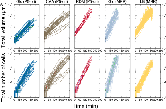
Supplementary Figure S1: Microcolony growth is exponential with respect to both total cell volume and cell number. Top panels: Plot of total cell volume over time for each microcolony in each growth condition. Each line represents a single field of view (from left to right $n=48,39,15,63,88$, and 109 fields of view). Bottom panels: total number of cells over time for the same experiments. Because filters tend to exclude many cells at the end of an experiment (because these cells might not finish dividing before the end of the experiment), the tracks shown here are for unfiltered data.

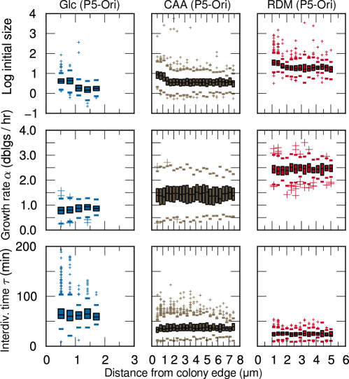
Supplementary Figure S2: Stability of measured parameters with respect to position of the cell in the microcolony. The plots are boxplots representing distributions, binned by distance of a cell from the microcolony edge (bin width is 0.3 $\mu$m). Top panel: logarithm of the initial volume $\log V_{0}$; the scored sizes are biased towards the colony edge, possibly because of the asymmetry of the image. Mid/bottom panel: the same bias is absent from measured interdivision times and individual-cell growth rates. The three colums refer to three different growth conditions.

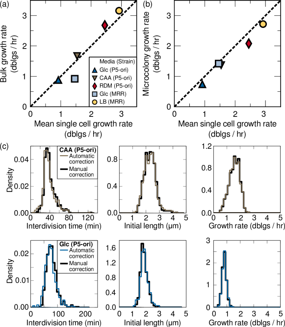
Supplementary Figure S3: Absence of biases from the segmentation/tracking analysis. (a and b) Growth rates of analyzed cells on agar pads are consistent with measured bulk and colony growth rates. (a) Correlation between bulk growth rate and the average growth rate in each condition. Symbols show the average across all biological replicate experiments. All conditions show close agreement between bulk and agar growth, except for the MRR strain in M9 + Glc; these differences are reproducible, and suggest the possibility of unexplored physiological differences between growth on agar and in bulk culture. Nevertheless, these differences do not significantly affect the mechanism of cell size control. (b) Comparison of the single-cell growth rate with the growth rate of individual microcolonies. The average single-cell growth rate (after all filters from the segmentation algorithm are applied) is compared to the average growth rate of microcolony area across each data set. Note that this growth rate is calculated without any filtering of cells due to the segmentation and tracking algorithm. The lines show $y=x$ as a guide to the eye. (c) Technical filters to correct for tracking errors do not bias the distributions of the main observables. The analysis compares the algorithm to to manually corrected data with the Schnitzcells software package (Young JW et al. Nature Protocols 7, 80–88, 2012). The resulting distributions of length, growth rate, and interdivision times are indistinguishable in the two cases. Top row shows the distributions for the P5 CAA condition, while the bottom row shows P5 Glc.

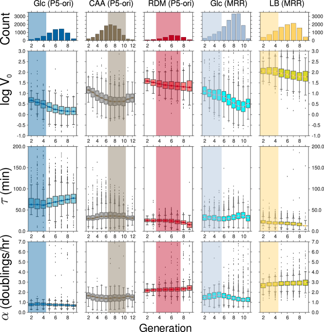
Supplementary Figure S4: Distributions of main observables for each growth condition binned by generation. Top row: total number of cells in each generation. Second row: distribution of log cell size for each generation. Third row: distribution of interdivision time $\tau$ for each generation. Bottom row: distribution of growth rate $\alpha$ for each generation. Trend lines represent the median. Box limits mark the inner quartile range ($IQR$). Whiskers extend to lowest and highest data point within $1.5\times IQR$ of the box boundaries. Vertical axes are common to all plots in a row. Box plot conventions are the same in all rows. The highlighted regions mark the filter on the range of generations with steadier growth used in further analyses.

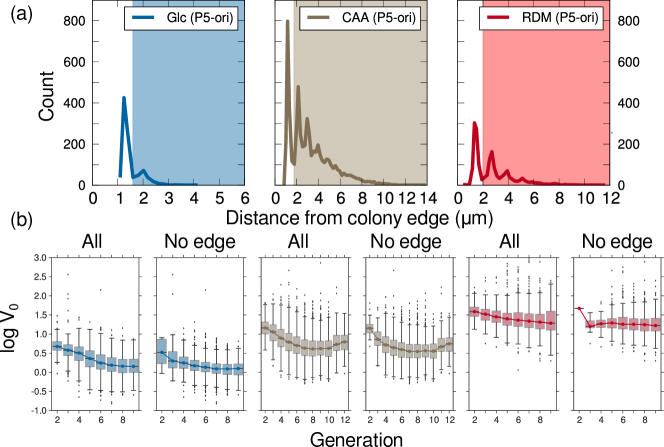
Supplementary Figure S5: Effects of colony edge segmentation bias on steadiness of initial cell size by generation. Top panel: overall distribution of minimal distances from colony edge in three different growth conditions. Shaded areas indicate filtered regions. Bottom panel: comparison of distributions of log initial size $\log V_{0}$ binned by generation (shown as boxplots as in figure S4), filtered to exclude cells on the colony edge (“no edge”) or unfiltered (“all”). These plots show that removing the cells close to colony edges improves the steadiness of initial size by generation, but does not fully account for the observed increasing trends in later generations.

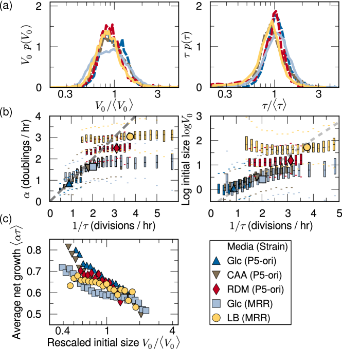
Supplementary Figure S6: All the results of this work are robust with respect to releasing the filter on generation range used in the main analysis (Fig. S4). The plots illustrate the main results without this filter applied. (a) Scaling of the initial size and doubling time distributions (Fig. 2). (b) Crossover in the fluctuations around the mean behavior and fluctuations around the Schaechter-Maaløe-Kjeldgaard plot (Fig. 4 and 5). (c) Scaling properties of size-growth plot (Fig. S12)

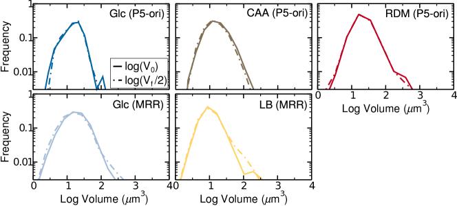
Supplementary Figure S7: The distribution of final sizes divided by two matches that of initial sizes. Distributions of initial size (dashed lines) or half the final size (solid lines) plotted for each growth condition (and suitably normalized). The good overlap in all conditions suggests that each population is in a nearly steady state of growth.

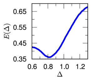
Supplementary Figure S8: Most parsimonious scaling collapse of the single-cell growth rate distributions is not at $\Delta=1$. To measure the goodness-of-collapse, a scaling exponent $\Delta$ is chosen and the histograms $p(\alpha)$ from each condition are rescaled according to $\alpha^{\Delta}p(\alpha)=F(\alpha/\langle\alpha\rangle^{1/(2-\Delta)})$ in order to obtain the curves $F$ as a function of the rescaled single-cell growth rate $\alpha/\langle\alpha\rangle^{1/(2-\Delta)}$. The functional $E(\Delta)$ is then defined as the total area of overlap between each pair of rescaled curves $F$ in the dataset, evaluated on their common support and normalized by the total number of overlapping pairs Giometto et al. (2013); Bhattacharjee and Seno (2001). The value of $\Delta$ for which $E(\Delta)$ is minimized is the most parsimonious scaling exponent; the uncertainty can be inferred from the width around the minimum. Unlike the most parsimonious scaling collapses for the interdivision time and initial size, the most parsimonious scaling collapse for the growth rate is $\Delta=0.82\pm 0.004$ (1% error).

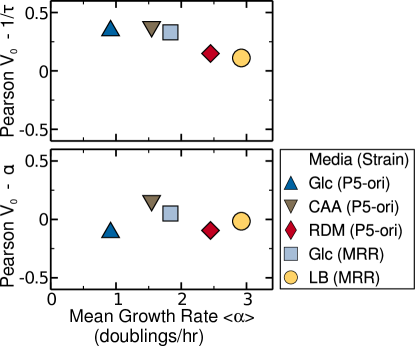
Supplementary Figure S9: Correlation between initial size and inverse interdivision time (top panel) or growth rate (bottom panel). Pearson correlation between the two quantities as a function of mean growth rate $\langle\alpha\rangle$.

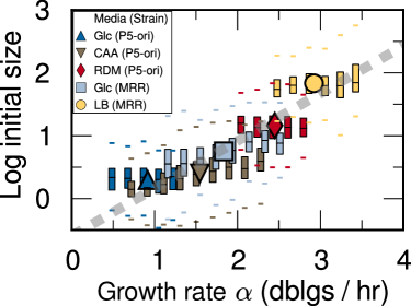
Supplementary Figure S10: Schaechter-Maaløe-Kjeldgaard plot of initial size as a function of growth rate, rather than inverse interdivision time (Fig. 5). Bin width is 0.2 doublings / hr. Large symbols represent population medians. Gray line is the fit of the population medians, with a slope of 66.3 minutes.

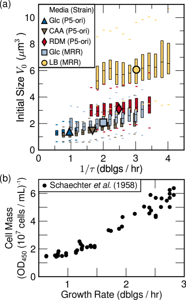
Supplementary Figure S11: Data is consistent with an exponential SKM law. (a) Plot of initial size (on a linear axis) as a function of inverse interdivision time (cf. Fig. 5(a), which plots size on a logarithmic axis). The trend in the mean is consistent with a super-linear dependence (e.g. exponential) dependence of size on $1/\tau$. Furthermore, the spread in size for a given value of $1/\tau$ increases with increasing values of $1/\tau$ (demonstrated by the increasing length of the boxes, which represent the interquartile range). However, perturbations of growth rate are limited in dynamic range, and thus these trends could also be consistent with other functional dependencies of size on $1/\tau$, such as a linear or polynomial dependence. (b) For comparison, the original data from the 1958 paper of Schaechter and coworkers Schaechter et al. (1958) plotting average cell mass versus bulk growth rate on linear axes. Each point represents the average of a culture growing in different nutrient conditions. Establishing the exact functional dependence of the SKM law is an open question, and alternate fits are possible also with the original Schaechter et al. data.

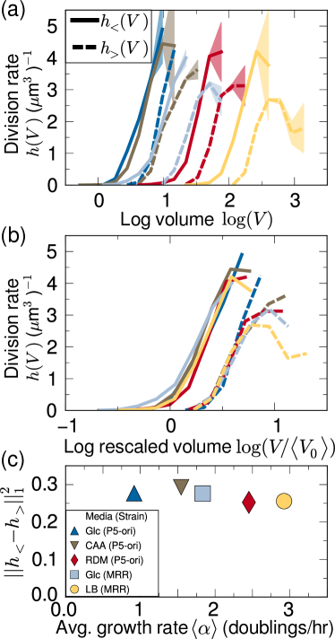
Supplementary Figure S12: Division control variations across different growth conditions are intimately linked to the universal size and doubling-time distributions, and consistent with a “concerted” control, where current size is not the only variable determining division. (a) Division (hazard) rates per unit volume conditional on initial size, plotted as a function of size alone. $h_{<}(V)$ (solid line) is the rate of cell division for cells whose initial size was smaller than the average initial size; $h_{>}(V)$ (dashed line) is the rate of cell division for cells whose initial size was larger than the average initial size. If size control depended only on current size then these curves should be the same. Shaded regions represent the standard error as in Wheals (1982). Colors represent different conditions as listed in the legend of (c). (b) As in (a) with size rescaled by average initial size. Error omitted for clarity. (c) $L_{1}$ distance between $h_{<}$ and $h_{>}$ on their common support, normalized by the length of the common support, and plotted as a function of growth rate.

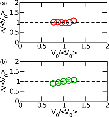
Supplementary Figure S13: Cell size change is consistent with an adder mechanism Campos et al. (2014); Taheri-Araghi et al. (2014). (a) The relative change in cell size (relative to initial size) plotted as a function of rescaled initial size for the MRR LB dataset. (b) Relative change in cell size plotted as a function of rescaled initial size for all data sets pooled together.

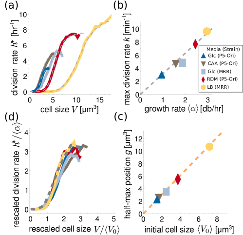
Supplementary Figure S14: Inference of division rate $h^{*}(V)$. (a) The dependence on cell size $V$ of the division rate $h^{*}(V)$ for cells growing in different conditions (see legend), thus with different average growth rate. The functional dependence is compatible with the results of the analysis of fast growing cells in a microfluidic device Osella et al. (2014). In particular, the division rate in every condition can be represented by a nonlinear saturating function $h^{*}=\frac{k}{1+(g/V)^{n}}$ (dashed lines) with a constant Hill coefficient $n$, while the other two parameters $g$,$k$ show a dependence on conditions. (b) Linear dependence of the maximum division rate on average growth rate $k=A\langle\alpha\rangle$. The values of the parameter $k$ are obtained by fitting the empirical division rates in (a) with a Hill function with $n=6$. (c) Direct proportionality between the half-maximum position of the division rate and the average cell size $g=B\langle V_{0}\rangle$. The $g$ values are obtained by fitting as in (b). (d) The division rates corresponding to different conditions collapse in a universal curve if the size is rescaled with its average value, and the division rate is rescaled with the corresponding average growth rate. Therefore, data from different strains and nutrient conditions can be in principle merged, if appropriately rescaled, and used to infer the universal division rate function (dashed line in the plot) with larger statistics.

).

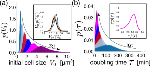
Supplementary Figure S15: Finite-size scaling in a sizer model, with Hill-function division hazard. (a) Histograms of initial size distributions obtained with direct simulations of the growth-division process for different values of $\langle\alpha\rangle$ (from 0.5 to 2 doublings per hour), using the two linear relations described in Fig. S14b,c to estimate the parameters of the division rate function. The inset shows how the model prediction corresponding to Eq. 29 (black line) well captures the empirical rescaled size distributions (same as Fig. 2a) (b) Histograms of doubling time distributions obtained with direct simulations as in (a). The inset shows that the finite-size scaling is predicted by the model also for the doubling time distribution. In fact, the distributions $p(\tau)\tau$ as a function of $\tau/\langle\tau\rangle$ perfectly collapse on a universal distribution. This distribution can not be quantitatively compared to the empirical ones in Fig. 2a, since concerted control is neglected in the model, resulting in broader and wrongly skewed predicted distributions of doubling times.

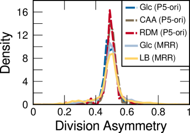
Supplementary Figure S16: Cell division is close to symmetric. Histograms of “division asymmetry” scores for cells. Division asymmetry is calculated from the initial lengths of a cell’s daughters according to $L^{D1}_{0}/(L^{D1}_{0}+L^{D2}_{0})$, where $L^{D1}_{0}$ is the initial length of daughter 1 and $L^{D2}_{0}$ is the initial length of daughter 2; a division asymmetry of 0.5 indicates that division was perfectly symmetric. In the P5-ori strain over 93% of cells in each condition have a division asymmetry between 0.4 and 0.6, suggesting close to symmetric division. This plots compares well to similar plots reported in other studies Campos et al. (2014); Taheri-Araghi et al. (2014); Soifer et al. (2014). The MRR strain had more division asymmetry (16-20% of cells had a division asymmetry score outside of the interval [0.4, 0.6]), perhaps due to a higher rate of filamentation in this strain.

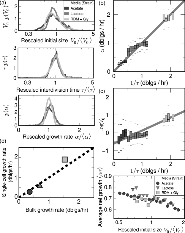
Supplementary Figure S17: The main results of this work are consistent with previously acquired data from different nutrient conditions. Data was taken and analyzed as described previously Kiviet et al. (2014) Nutrient conditions: M9 + Acetate, M9 + Lactose, and Neidhardt’s Rich Defined Media (RDM) + Glycerol, spanning growth rates from between $\approx 0.25$ to $\approx 1.8$ doubling per hour Kiviet et al. (2014). Each data set has between 500-1000 cells. (a) Rescaled histograms of initial size $V_{0}$ (top), interdivision time $\tau$ (middle) and growth rate $\alpha$ (bottom), as in Figs 2 and 3. (b) Correlation between growth rate $\alpha$ and inverse interdivision time, binned by $1/\tau$ (cf. Fig. 4a). (c) Shaechter-Maaløe-Kjeldgaard plot (top) showing correlation between log initial size and inverse interdivision time (cf. Fig. 5a), and Average net growth $\alpha\tau$ binned by log initial size (bottom, cf. Fig. 5d). (d) comparison of bulk and agar growth rates (cf. Fig. S3).

Supplementary Tables

Data set	P5-ori			MRR
	Glc	CAA	RDM	Glc	LB
Segmentation and tracking algorithm
Objects touch border or beginning/end of moviea	456	7,725	812	14,578	7.136
Unsuccessful trackingb	10,203	7,882	7,167	35,608	35,000
Unsuccessful tracking / estimated cells +	6,428	5,178	3,705	28,842	15,225
No motherc	127	422	2	6	28
Negative growth rate	22	14	9	236	85
Low $r^{2}$ valued	398	517	147	1,644	580
Division time $<8.6$ minf	0	28	78	6	23
Final	5,765	10,802	2,579	19,564	9,489
Steadiness filters
Restriction of the interval of generations considerede	4,803	4,897	744	16,861	7,839
Final	962	5,905	1,835	2,703	1,650

Supplementary Table S1: Summary of the effects of data-analysis filters. Each row of the table counts the objects ^a Excluded objects were touching the border of the image for at least one frame, or were present at either the start or the end of the move, precluding assignment of initial or final size. ^b Excluded objects were lost for at least a frame during tracking due to image segmentation errors. This was often due to cells being lost for a frame which disrupted tracking. Importantly, most of these excluded tracks artificially inflate the number of objects excluded with respect to the number of excluded cells; for example, if the track of a single cell is interrupted 3 times during its cell cycle, then 4 objects representing the same cell is discarded by the filter. ⁺ Estimate of the number of cells excluded by this filter as the number of excluded objects times the ratio of the average track length for excluded objects relative to passing objects. ^c Not assigned a mother by the tracking algorithm, due to errors in segmentation. ^d Growth of excluded cells with a goodness-of-fit ($r^{2}$) to an exponential of less than 0.8. Excluded objects were typically incorrect segmentations lasting several frames, affecting estimated size and growth rate. ^e Cells were restricted by generation based on examination of the steadiness of the data set (see Fig. S4 and S6). ^f Exclusion of track lengths shorter than 8.6 minutes (see Methods for an explanation). This filter impacts very few objects.