Nonextensive Statistical Analysis of Meteor Showers and Lunar Flashes

Abstract

The distribution of meteor magnitudes is usually supposed to be described by power-laws. However, this relationship is not able to model the whole data set, and the parameters are considered to be dependent on the magnitude intervals. We adopt a statistical distribution derived from Tsallis nonextensive statistical mechanics which is able to model the whole magnitude range. We combined meteor data from various sources, ranging from telescopic meteors to lunar impactors. Our analysis shows that the probability distribution of magnitudes of IMO and MORP data are similar. The distribution of IMO visual magnitudes indicates that $2.4\pm 0.5\%$ of the meteors of a shower may be telescopic ($m>6$). We note that the distribution of duration of lunar flashes follows a power-law, and a comparison with the distribution of meteor showers suggests the occurrence of observational bias. The IMO sporadic meteor distribution also seems to be influenced by observational factors.

1 Introduction

Meteor showers are phenomena resulting from the collision of meteoroid streams with the Earth’s atmosphere. These particles originated from comets and asteroids, generically known as parent-bodies. The first dynamic association between a comet and a meteor shower was established in 1867 involving the Leonids and 55P/Tempel-Tuttle (Manson, 1995). A similar connection between the asteroid (3200) Phaethon and the Geminids meteor shower was established more than a century later (Whipple, 1983). Studies of the physical properties of meteor showers began in the second half of the nineteenth century. These studies were focused on determining the chemical properties and brightness of meteors (Millman, 1980). The mass cumulative distribution of a meteor shower is usually assumed to be represented by an exponential function (Zolensky et al., 2006),

$$\log N=A\log M+B,$$ (1)

where $M$ is the meteoroid mass, $A$ is the integrated mass index, $B$ is a constant, and $N$ is the meteor flux (number of events per area per time) with mass equal or greater than $M$. The cumulative distribution of meteor magnitudes $m$ is given by Baggaley (1977)

$$N_{m}=Cr^{m},$$ (2)

where $N_{m}$ is the number of meteors brighter than, or equal to, $m$, $r$ is the ratio between the number of meteors with magnitudes $m$ and $m+1$, and $C$ is a constant. Equations (1) and (2) do not properly model all the mass distribution and magnitudes of a meteor shower. This is particularly significant for meteors with $m\leq-3$. Specifically, there is a variation of the mass index for these magnitudes. The use of Equation (1) can infer an incorrect estimate of the mass flow incident on the Earth. An empirical solution usually adopted for this problem is to use Equation (1) for specific mass intervals, instead of assuming that it is valid for the whole distribution. A fragmentation process can occur during formation, in the transit of meteoroids between the parent-body and the Earth, or its interaction with the Earth’s atmosphere (Tóth & Klačka 2004; Ceplecha & Revelle 2005; Jenniskens & Vaubaillon 2007). The frequency of meteoric bombardment on the Moon is presumably similar to that on the Earth. This seems quite reasonable, given the size of a few million kilometres of meteoroid streams associated with annual showers (Nakamura et al., 2000). The visualisation of the collision of meteoroids with the Moon is an unusual phenomenon. The only known records, until the 1990s, were associated with more energetic events than those commonly observed on Earth. An example is the photographically recorded flash by Stuart (1956). Based on the obtained image, Buratti & Johnson (2003) estimated that a body of 20 m of diameter crashed on the Moon, creating a 1.5 km diameter crater. The detection of lunar impacts was not possible until the introduction of CCD’s cameras into this type of observation, due to the short duration and low brightness of the events (Ortiz et al., 2002). The first detection of lunar flashes was obtained by Bellot Rubio et al. (2000) and Dunham et al. (2000) for the Leonids meteor shower. The impacts can be associated with bodies with a mass on order of a few kilograms. The detection of these events is subject to a combination of factors such as moon phase, instruments used, and the nature of the meteoroid. This ensemble of physical and instrumental factors is called observational bias. Observational bias is particularly important in the study of meteors and related phenomena (Hawkes & Jones, 1986). As for the parameters associated with lunar flashes, Tost et al. (2006) concluded that most impacts have a typical duration and magnitude from 0.1 to 0.5 s and $m\sim 10$ respectively. Davis (2009) developed a model for the plume of steam due to an impact on the Moon, which suggests that parameters such as brightness and duration of the event are proportional to the mass and kinetic energy of the meteoroid. Bouley et al. (2012) found a direct correlation between the magnitude and duration of the flashes. However, this relationship does not appear to be valid for the Leonids. The difference between Leonids and other meteor showers is likely explained by the higher velocity of this swarm. Models that describe distributions associated with lunar flashes are not yet available in the literature. Such models are important for the identification of the observational bias, and to verify whether the incidence of meteoroid streams on the Moon are consistent with those observed on the Earth. We use nonextensive distributions, that emerge from Tsallis statistics (Tsallis 1988, 2009) to analyse data from meteor surveys and lunar flashes. In particular, we verify that the nonextensive distribution proposed by Sotolongo-Costa et al. (2007) models quite well the cumulative magnitude distribution of meteor showers. For the lunar impacts, the duration of the steam plumes is modelled by a power-law distribution. The correlation between the predictions in both data sets suggests that there is a significant difference in the distribution of sporadic meteors and those associated with a shower. Similarity in the distributions suggests a uniformity of the physical processes that govern the fragmentation of meteoroids and the formation of lunar flashes. The presence of observational bias is suggested in the data of meteors showers and lunar flashes.

2 Nonextensive Distributions of Meteor Showers and Lunar Flashes

Boltzmann-Gibbs (BG) statistical mechanics needs the assumption (among others) of short-range interaction between particles, that implies strong chaos at the microscopic level and eventually results in the ergodic hypothesis. Distributions that emerge from BG formalism are based on the exponential function, that has rapidly decaying tails, and thus events far from the expectation values are utterly rare. Long-range gravitational interaction does not satisfy this basic assumption, and application of the statistical mechanics formalism to self-gravitating systems results in difficulties and/or inadequacies, e.g., negative specific heat, non-equivalence of ensembles (Lynden-Bell & Wood 1968; Thirring 1970; Landsberg 1990; Padmanabhan 1990). These inadequacies have been at least partially overcome by the use of nonextensive statistical mechanics, that is a generalisation of BG formalism (i.e., BG statistics is a particular case of nonextensive statistics). Nonextensive distributions present tails that are asymptotically power-laws, which implies that rare events, though unlikely, do not have vanishingly small probabilities. The generalisation is governed by the entropic index $q$, that controls the power-law regime of the tails; the particular value $q=1$ recovers the usual BG formalism. Non-Boltzmannian distributions, negative specific heat, and compatibility with nonextensive statistical mechanics have been computationally verified (Latora et al. 2001; Borges & Tsallis 2002; Tsallis et al. 2007). Examples linking nonextensivity to astrophysical systems are galore. We point out three instances that ranges from small bodies in the Solar System, spherical galaxies, and the whole universe: nonextensive distributions in asteroid rotation periods and diameters have been observed (Betzler & Borges 2012). Models for distribution function for spherical galaxies have been proposed, and density profiles have been shown to be a nonextensive equilibrium configuration, that can be used to describe dark matter haloes. The M33 rotation curve has been successfully fitted within this context (Cardone et al. 2011). Small deviations from Gaussianity of the cosmic microwave background temperature fluctuations have also been verified, and nonextensive distributions seem to properly describe the data by the Wilkinson microwave anisotropy probe (Bernui et al. 2006). More examples of applications of nonextensive statistical mechanics in astrophysical systems may be found in Tsallis (2009).

Fragmentation models have benefited from developments in material science, combustion technology and geology, among others. Some attempts to obtain the size distribution function were made using the principle of maximum entropy (Li & Tankin 1987, Sotolongo-Costa et al., 1998). The expression for the BG entropy, in its continuous representation, is given by

$$S=-k\int p(x)\ln p(x)\,dx,$$ (3)

where $p(x)$ is the probability of finding the system in a specific microscopic state, generically represented by the dimensionless coordinate $x$, and $k$ is the Boltzmann’s constant, that guarantees dimensional consistency to the expression - we may take here $k\equiv 1$ without loss of generality. BG entropy is valid when short-range interactions are present. A fragmented object may be considered as a collection of parts that have entropy larger than the original (Sotolongo-Costa et al., 2007) ($S(\cup A_{i})>\sum_{i}S(A_{i})$). This suggests that it may be necessary to use a nonadditive entropy, rather than the additive BG entropy. Tsallis nonadditive entropy for the distribution of mass fragments is written as

$$S_{q}=k\frac{1-\int_{0}^{\infty}{p^{q}}(M)\,dM}{q-1},$$ (4)

where $M$ is a dimensionless mass, $q$ is the entropic index, and $p(M)$ is the probability density of a fragment to have mass between $M$ and $M+dM$. Maximisation of Equation (4), constrained to the normalisation condition

$$\int_{0}^{\infty}p(M)\,dM=1,$$ (5)

and to the $q$-expectation value of the mass

$$\int_{0}^{\infty}M{p^{q}}(M)\,dM=\langle M\rangle_{q},$$ (6)

$\langle M\rangle_{q}$ is the generalised $q$-expectation value, according to Curado & Tsallis (1991) (see also Tsallis et al. (1998) for a broader view of the generalisation of the constraints) leads to the mass probability density of a meteor shower

$$p(M)dM=a(1+bM)^{-\frac{1}{q-1}}dM.$$ (7)

Normalisation condition, Equation (5), imposes that $a=b(2-q)/(q-1)$. The inverse cumulative distribution $P_{\geq}(M)=N_{\geq}(M)/N_{t}=\int_{M}^{\infty}p(M^{\prime})\,\mathrm{d}M^{\prime},N_{\geq}(M)$ is the cumulative number of meteors with mass equal to or greater than $M$, and $N_{t}$ is the total number of meteors, leads to

$$N_{\geq}(M)=N_{t}(1+bM)^{\frac{2-q}{1-q}}=N_{t}[\exp_{q}(-\beta M)]^{2-q}$$ (8)

$(b=(q-1)\beta)$, that is identified with a $q$-exponential, defined as

$$\exp_{q}x\equiv[1+(1-q)x]^{\frac{1}{1-q}},$$ (9)

if $[1+(1-q)x]>0$, and $\exp_{q}x\equiv 0$ if $[1+(1-q)x]\leq 0$ (Tsallis, 1994). This expression provides, in the asymptotic limit, a power-law regime

$$N(M)\sim M^{-n}$$ (10)

with $n=\frac{2-q}{q-1}$, similar to Equation (2). Once the relation between the magnitude and meteor mass can be expressed by an exponential function (Jacchia et al. 1965), we adopt the expression used by Sotolongo-Costa et al. (2007)

$$M=M_{0}{e^{-\gamma m}},$$ (11)

where $M_{0}=M(m=0)$, and $\gamma$ is a constant. Following their lines, taking into account that

$$p(m)dm=p(M)dM,$$ (12)

and finally integrating between $m$ and $-\infty$, to obtain the inverse cumulative distribution, we get

$$N_{\geq}(m)=N_{t}[\exp_{q}(-\beta_{m}e^{-\gamma m})]^{2-q}$$ (13)

($\beta_{m}=\beta M_{0}$; $\beta_{m}$ is taken as a fitting parameter in our procedure). The power of a $q$-exponential can easily be rewritten as another $q$-exponential, with a different index $q^{\prime}$:

$$N_{\geq}(m)=N_{t}\exp_{q^{\prime}}(-\beta^{\prime}_{m}e^{-\gamma m})$$ (14)

with $\frac{1}{1-{q^{\prime}}}$=$\frac{2-q}{q-1}$ and $\beta^{\prime}_{m}=(2-q)\beta_{m}$. Graphical representation of Eq. (14) with the ordinate in logarithm scale ($\log$ with base 10), and the abscissa (magnitude) in linear scale, as shown in the main panel of Figures 1–3, presents two main regimes. For highly negative magnitudes (i.e., bright objects), Eq. (14) displays an ascending straight line with slope given by $\gamma/(q^{\prime}-1)\log_{10}e$ (the rare events region). For high values of magnitudes, the cumulative distribution tends to its upper value $N_{t}$, and the semi-log plot exhibits a quasi-flat region. Elongation of the ascending straight line of the rare events region intercepts the horizontal line of the quasi-flat region at the transition point between regimes, $m^{*}=\frac{1}{\gamma}\ln[(q^{\prime}-1)\beta^{\prime}_{m}]$. A similar twofold behaviour occurs regarding the decreasing $q$-exponential distribution, as explained in Betzler & Borges (2012), and illustrated by its Fig. 1. We have gathered data from meteor showers, and fitted Equation (14) (it is to be shown in the following sections).

3 Observational Data

The cumulative distributions of meteor showers were obtained from the counting of meteors in the range of visual magnitude, provided by the International Meteor Organization (IMO) (available at the VMDB – Visual Meteor Database, http://www.imo.net/data/visual). In this analysis, we consider meteor magnitudes ranging from $-6$ to $+6$ with an interval of one magnitude between the classes. The analysed counting was originated from observers that rated the local sky with limiting magnitude $lm\geq 5.5$. This selection criterion has been adopted in similar studies (Brown & Rendtel 1996, Arlt & Rendtel 2006), and it aims to minimise observational bias. We analysed 10 showers: Geminids (GEM), Orionids (ORI), Quadrantids (QUA), Eta Aquariids (ETA), Lyrids (LYR), Capricornids (CAP), Leonids (LEO), Perseids (PER), Alpha Monocerotids (AMO), Southern Taurids (STA) and also sporadic meteors (SPO). The choice of these showers is associated with the variety of physical and dynamic characteristics of each meteoroid stream, which is possibly associated with the differences in their parent bodies. In order to verify whether the parameters of Equation (14) have a temporal variation, we have analysed the whole observed meteors in the years 2000, 2002, 2004, 2006, 2008 and 2010 (data from VMDB) according to the limit magnitude criterion above mentioned. Additionally, for the LEO, we have analysed the distribution of meteors in the 1999’s outburst. To verify if any trends detected within the VMDB data are valid, we analysed panchromatic magnitudes of fireballs, recorded by the Meteor Observation and Recovery Project (MORP) survey (Halliday et al., 1996). From this data set, we studied the SPO, PER and STA fireballs. Specifically, the PER and STA have presented the largest number of observations in the showers’ database. To demonstrate the possible occurrence of systematic errors between visual, photographic and TV data, we compared the VMDB and MORP distributions with those detected by a TV camera installed in Salvador (SSA, Bahia, Brazil). The camera uses a CCD 1/3 inch Sony Super HAD EX View. This instrument is pointed towards the zenith, and has a field of 89 degrees. The 49 SPO meteors detected were observed between July and October, 2011. The meteor magnitudes were estimated using the method of Koten (1999). With the same purpose, the SPO MORP magnitude distribution have been compared with the Fireball Database Center (FIDAC) data set (Knöfel & Rendtel, 1988) obtained in the years 1993, 1994, 1995, 1996 and 1997, taken from “Fireball Reports 1993–1996” (available at http://www.imo.net/fireball/reports).

We only considered the highest luminosity of detected meteors from the MORP and SSA data. This procedure was adopted to allow a comparison with VMDB and FIDAC visual data. Visual observers generally record only the brightness peak of a meteor (Beech et al., 2007). The duration of lunar flashes were collected by the Automated Lunar and Meteor Observatory (ALaMO) of NASA’s Meteoroid Environment Office. The analysed data were obtained between 2005 and 2010. Instrumental characteristics of this initiative are presented in Suggs et al. (2008). We obtained the distribution of the duration of lunar flashes of SPO and LEO, GEM, LYR, Taurids (TAU), ORI and QUA showers. The duration of the flashes were obtained by multiplying the number of frames in which the events are recorded by $1/30$ s, that corresponds to the integration time of the TV cameras used at the ALaMO.

4 Processing and analysis

The data from ALaMO, FIDAC, VMDB MORP and SSA were separately displayed in a crescent cumulative distribution. It was found that ALaMO, FIDAC, MORP and SSA data are best described by a power-law (Equation (10)). Data from VMDB and SPO MORP, which present a greater magnitude range than the other sources, are were better fitted by Equation (14) (details are presented in the following sub-sections 4.1 and 4.2). The parameters were determined with the line search strategy, and the search direction was obtained with the conjugate gradient method. The adequacy of the fittings, as well as the similarity between distributions, was established by the Pearson‘s’ chi-square test. All fittings present confidence level equal to or greater than $95\%$.

4.1 Meteor Showers

We have verified that Equation (14) satisfactorily fits all VMDB meteor showers, and also the SPO (see Fig. 1, with PER, that was chosen as a representative sample because it is one of the most constant and best observed showers (Beech et al., 2004)). We have obtained mean values of $q=1.57\pm 0.05$ ($q^{\prime}=2.3\pm 0.3$) and $\gamma=1.1\pm 0.2$. The coincidence of the values of $q$ for different showers suggests that the fragmentation process that acts on VMDB meteors are essentially the same for the whole sample. Specifically, the value $q>1$ implies that there are other effects that influence these distributions besides short-range force.

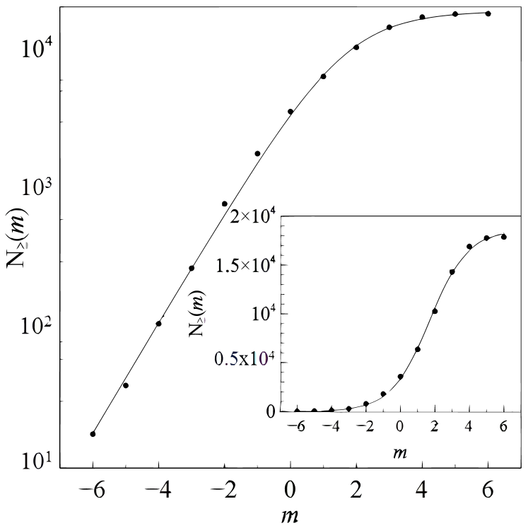
Figure 1: Cumulative distribution $N_{\geq}(m)$ $\times$ magnitude $m$ of PER (2000) (circles), and fitting with Equation (14), $N_{t}=18660$, $\beta^{\prime}_{m}=4.42$, $\gamma=0.879$, $q^{\prime}=1.97$. Main panel: semi-log scale; inset: linear scale.

We have established that $97.6\pm 0.5\%$ of VMDB meteors have magnitudes $m\leq 6$. The rest are telescopic meteors. The counting of telescopic meteors from PER, ORI, and LEO by Porubčan (1973) is much smaller than the present prediction. This suggests that our result may be taken as an upper bound for the number of meteors with $m>6$.

We did not detect any temporal variation in the probability distribution of meteors. We have compared VMDB data from the year 2000 with the equivalent data obtained up to the year 2010. Specifically for LEO, the counting of meteors belonging to the 1999 storm were compared with those from 2000 to 2010. The temporal independence was also verified. We have concluded that, despite the possibility of a seasonal increase in the total number of meteoroids ($N_{t}$), the mass distribution in a meteor shower remains constant. As a consequence of the invariance of the distributions along time, we found that the meteor distribution may be established using sparse data of several years. This hypothesis has been tested using all data from 2000 to 2010 of the CAP shower, and they are well adjusted by Equation (14). Probability distribution of the CAP is similar to the distributions of other showers (see Fig. 2). When the showers were separately analysed by their parent bodies, we find that there are no differences between the meteor distributions that originate from comets or from asteroids. This test was done by comparing the distributions of the ORI and ETA (1P/Halley) and GEM (3200 Phaethon) and QUA (2003 EH1, Jenniskens 2004). The probability distributions of showers associated with comets do not differ when they are separated by their dynamic characteristics. To this end, we have compared the data showers associated with the Halley Family (ETA), the Jupiter Family (LEO), and with long period comets (LYR). The only difference that we were able to detect in the VMDB data is between SPO meteors and those of all the other showers (see Fig. 3).

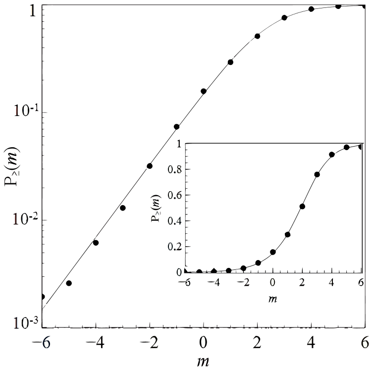
Figure 2: Cumulated probability distributions of CAP (2000-2010) (circles) and fitting with Equation (14) with $P_{\geq}(m)=N_{\geq}(m)/N_{t}$), $N_{t}=1536$, $\beta^{\prime}_{m}=10.20$, $\gamma=1.13$, $q^{\prime}=2.42$ (solid line). Main panel: semi-log scale; inset: linear scale.

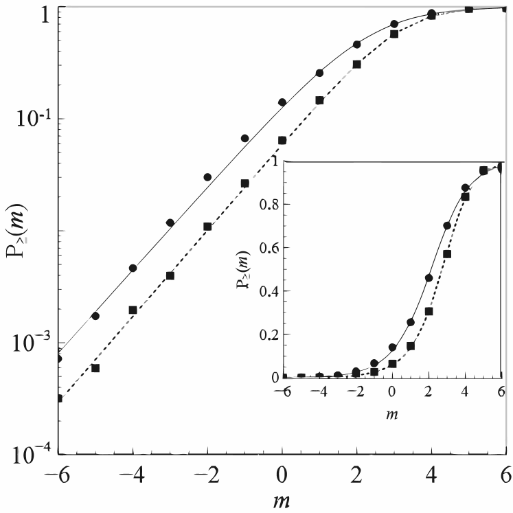
Figure 3: Cumulated probability distributions of LEO (1999) (circles) and SPO (2004) (squares), and their corresponding fittings (Eq. (14)) with $N_{t}=60329$, $\beta^{\prime}_{m}=8.72$, $\gamma=0.99$, $q^{\prime}=2.16$ (LEO, solid line) and $N_{t}=21942$, $\beta^{\prime}_{m}=48.1$, $\gamma=1.34$, $q^{\prime}=2.52$ (SPO, dashed line).

The difference between the SPO and shower probability distributions is maximum for the magnitude 2 (Fig. 4). In this range, there are $\sim 20$% more meteors in the showers than observed in SPO. The difference is negligible for the magnitudes $-6$ and $+6$. This difference may be associated with observational bias in the process of data collection. We have found that most observations of annual showers occur $5\pm 2$ days before or after the peak of the event. For instance, in the year 2010, VMDB presents 834 entries of SPO ($lm\geq 5.5$), and 434 of those ($\cong 52\%$) correspond to the peak period for PER, August, 05–19. 1523 PER entries were recorded during this period. This may be evidence that the sky is not systematically monitored except in the annual shower seasons. The occurrence of observational bias in the VMDB SPO data was also suggested when we analysed the data from the MORP survey. The MORP fireballs associated with STA and PER showers were modelled by Equations (10) and (11) (Fig. 6).

The comparison between modelled distributions suggested that these showers are similar. SPO data, however, are modelled by Equation (14), possibly due to the magnitude range of this sample (Fig. 7). The modelled distributions of showers are not correlated to the observed distribution of the SPO. The number of SPO meteors in the considered magnitude interval is systematically greater than that observed in the showers, and this is a known result (Pawlowski et al. 2001, Rendtel 2006). We obtained $q=1.51\pm 0.03$ for the MORP data.

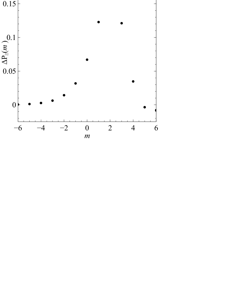
Figure 4: Difference between cumulated probabilities of LEO (1999) and SPO (2004), ${\Delta}P_{\geq}(m)=P_{\geq}^{\text{LEO}}(m)-P_{\geq}^{\text{SPO}}(m)$, as a function of the magnitudes $m$, putting in evidence the maximum discrepancy at $m=2$.

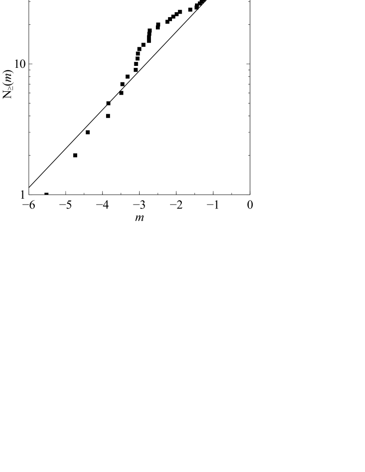
Figure 5: Cumulative distribution $N_{\geq}(m)$ $\times$ magnitude $m$ of meteors detected by an all sky camera at Salvador (SSA, squares). Solid line represents Equations (10) and (11) ($n=1.2$ e $\gamma=0.59$). The magnitude error is 0.4. Fitting is not good for magnitudes around $m=-2$.

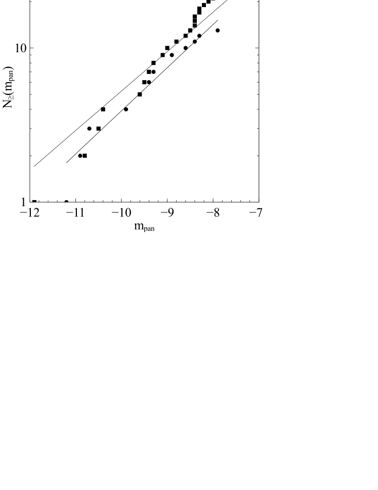
Figure 6: Cumulative distribution of the number of meteors MORP $N_{\geq}(m_{\text{{pan}}})$ $\times$ panchromatic magnitude $m_{\text{pan}}$, STA (squares), PER (circles) and their corresponding fittings (Eq.s (10) and (11)), STA (solid line, $n=0.83$) and PER (dashed line, $n=0.91$). Both fittings using $\gamma=0.83$ calculated from MORP-SPO data.

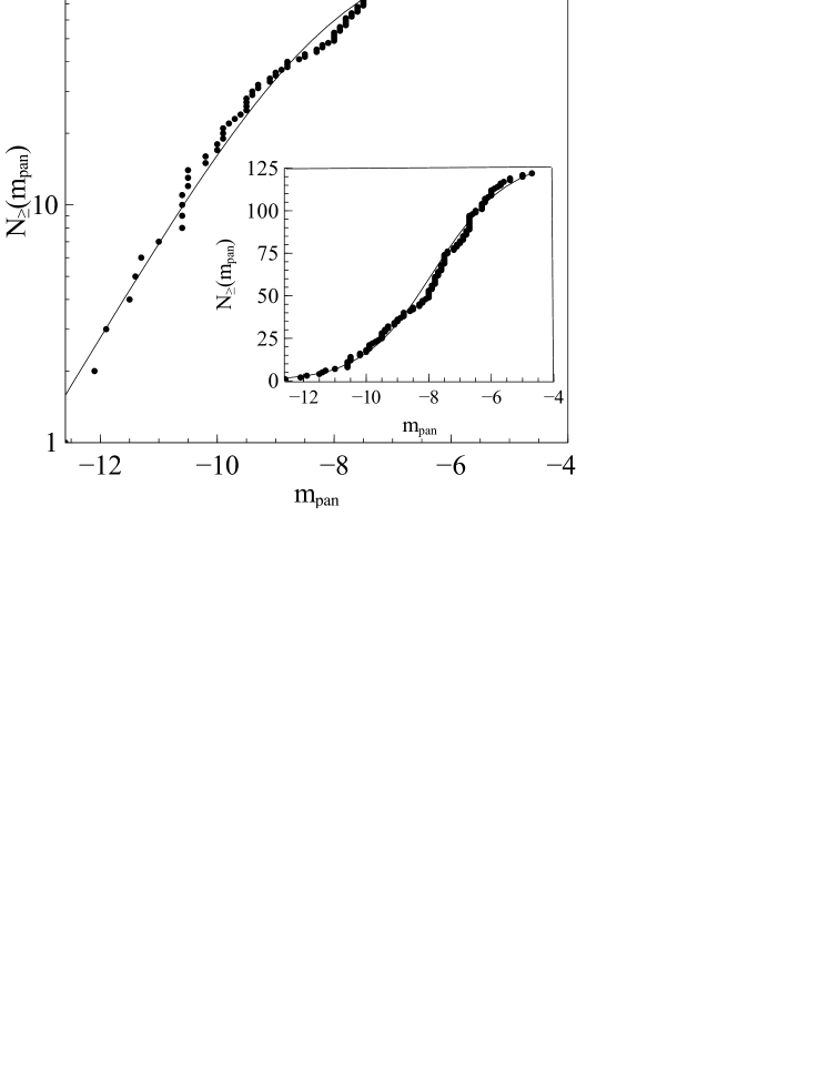
Figure 7: Cumulative distribution of the number of meteors MORP $N_{\geq}(m_{\text{{pan}}})$ $\times$ $m_{\text{pan}}$, MORP-SPO (circles). and fitting with Equation (14), $N_{t}=131$, $\beta^{\prime}_{m}=0.0015$, $\gamma=0.83$, $q^{\prime}=1.86$ (solid line). Main panel: semi-log scale; inset: linear scale.

The SSA data are well fitted with Equations (10) and (11). The value obtained is $q=1.46\pm 0.04$ (see Fig. 5). The FIDAC’s data were also adjusted by Equation (10) and (11), with $q=1.8\pm 0.1$ (Fig. 8). We have found that the FIDAC apparent magnitudes have good adherence to the model. The same is not true for zenithal magnitude distribution. This lack of agreement with the model is associated with the transformation of apparent to zenithal magnitudes. This conversion takes into account an estimate of the fireball altitude. The estimate of this parameter can cause the introduction of an additional source of error, as suggested by Bellot Rubio (1995). This problem is particularly important for fireballs brighter than magnitude $-6$. We have verified the occurrence of a temporal variation in the distribution of apparent magnitudes comparing the data from 1993 to 1997. The compatibility only occurs when we consider a range of magnitudes between -6 and -3. This suggests the occurrence of observational bias in the FIDAC sample. This bias may be associated with the difference of the terrestrial surface area covered by the surveys, total duration of the observations and field of view. Considering these factors, a compatibility was obtained by Zotkin & Khotinok (1978) comparing visual data of fireballs observed in the former Soviet Union with meteor photographic networks. For the same reason, this compatibility also does not occur between the MORP and SSA data.

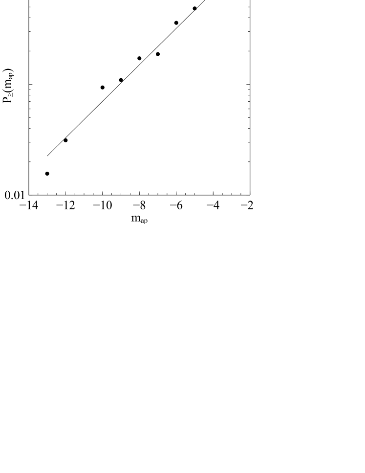
Figure 8: Cumulated probability of FIDAC $P_{\geq}{(m_{\text{{ap}}})}$ $\times$ apparent magnitude $m_{\text{ap}}$ (data from file FIDAC95.001) Solid line, Eq.s (10)–(11), with $n=0.33$ and $\gamma=1.1$.

4.2 Lunar Flashes

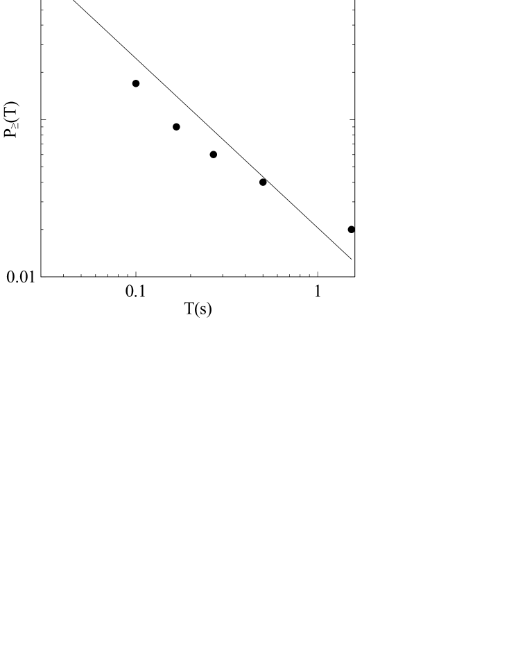
Figure 9: Cumulative probability for the duration $T(s)$ of ALaMO lunar flashes for SPO (circles). The solid line corresponding the fitting of Eq. (10) with $n=1.6$.

ALaMO’s data are modelled by Equation (10) for the impact durations (Fig. 9). Distributions for the LEO, LYR and GEM showers are similar (this corresponds to half of the analysed sample), and this is not observed for the other showers. On the other hand, it would be expected that SPO distribution differs from the shower distributions, but we have observed that SPO distribution present similarities with ORI, GEM, LYR and LEO. These results disagree with the conclusions obtained with the VMDB and MORP data. This suggests the occurrence of observational bias in the data set, that can be connected to inadequate observation conditions, such as the occurrence of unfavourable Moon phases for the detection of the flashes, and/or bad weather. Due to bias, it is not possible to infer the existence of lunar flashes with duration less than 0.033 s. The mean value for the similar meteor showers is $q=1.32\pm 0.02$, and this value is close to the one obtained by photometric data. Since both phenomena are supposedly directly associated to the meteoroid masses, we can conclude that the showers distributions observed on the Earth and on the Moon are compatible. As in the case of meteor showers, we suppose that the mechanisms that govern the duration of lunar flashes are both short- and long-range in nature.

5 Conclusions

We analysed the distribution of magnitudes of meteors and duration of lunar flashes through nonextensive statistics. We used data from various sources that cover a wide range, from telescopic meteors to lunar impactors. Our main conclusions are as follows:

1. The cumulative distribution of the magnitudes of the meteors is well represented by a $q$-exponential. This distribution is valid for meteoroids of masses varying from telescopic meteors to lunar impact bodies. A power-law, that is the asymptotic limit of the $q$-exponential, is observed for smaller intervals of masses.

2. We estimate that $2.4\pm 0.5\%$ (upper bound limit) of meteoroids in meteors showers are telescopic ($m>6$).

3. The cumulative distributions of all meteor showers registered in VMDB and MORP datasets are similar, independent of time, independent of the type of parent body (whether asteroid or comet) or its dynamic family.

4. In the distributions of sporadic (non-shower) meteors the VMDB may present observational bias. For instance, the probability of occurrence of meteors of magnitude 2 in showers is about $20\%$ higher than the equivalent in SPO.

5. The cumulative distribution of duration of lunar flashes registered by ALaMO is modelled by a power-law. The analysis of the distributions suggests that the meteor showers observed on the Earth and on the Moon are compatible.

References

- Arlt & Rendtel (2006) Arlt R., Rendtel J., 2006, MNRAS, 367, 1721
- Baggaley (1977) Baggaley W. J., 1977, MNRAS, 180, 89
- Beech et al. (2004) Beech M., Illingworth A., Brown P., 2004, MNRAS, 348, 1395
- Beech et al. (2007) Beech M., Nie W., Coulson I. M., 2007, JRASC, 101, 139
- Bellot Rubio (1995) Bellot Rubio L. R., 1995, A&A, 301, 602
- Bellot Rubio et al. (2000) Bellot Rubio L. R., Ortiz J. L., Sada P. V., 2000, EM&P, 82, 575
- Bernui et al. (2006) Bernui A., Tsallis C., Villela T., 2006, Physics Letters A, 356, 426, astro-ph/0512267, ADS
- Betzler & Borges (2012) Betzler A. S., Borges E. P., 2012, A&A, 539, A158
- Borges & Tsallis (2002) Borges E. P., Tsallis C., 2002, Phys A, 305, 148, cond-mat/0109504
- Bouley et al. (2012) Bouley S., Baratoux D., Vaubaillon J., Mocquet A., Le Feuvre M., Colas F., Benkhaldoun Z., Daassou A., Sabil M., Lognonné P., 2012, Icar, 218, 115
- Brown & Rendtel (1996) Brown P., Rendtel J., 1996, Icar, 124, 414
- Buratti & Johnson (2003) Buratti B. J., Johnson L. L., 2003, Icar, 161, 192
- Cardone et al. (2011) Cardone V. F., Leubner M. P., Del Popolo A., 2011, MNRAS, 414, 2265, 1102.3319, ADS
- Ceplecha & Revelle (2005) Ceplecha Z., Revelle D. O., 2005, MAPS, 40, 35
- Curado & Tsallis (1991) Curado E. M. F., Tsallis C., 1991, J. Phys. A, 24, L69
- Davis (2009) Davis S. S., 2009, Icar, 202, 383
- Dunham et al. (2000) Dunham D. W., Sterner II R., Gotwols B., Cudnik B. M., Palmer D. M., Sada P. V., Frankenberger R., 2000, Occultation Newsl., 8, 9
- Halliday et al. (1996) Halliday I., Griffin A. A., Blackwell A. T., 1996, M&PS, 31, 185
- Hawkes & Jones (1986) Hawkes R. L., Jones J., 1986, QJRAS, 27, 569
- Jacchia et al. (1965) Jacchia L. G., Verniani F., Briggs R. E., 1965, Smithson. Astrophys. Obs. Spec. Rep., 175
- Jenniskens (2004) Jenniskens P., 2004, AJ, 127, 3018
- Jenniskens & Vaubaillon (2007) Jenniskens P., Vaubaillon J., 2007, AJ, 134, 1037
- Knöfel & Rendtel (1988) Knöfel A., Rendtel J., 1988, JIMO, 16, 186
- Koten (1999) Koten P., 1999, in Baggaley W. J., Porubcan V., eds, Meteroids 1998 Photometry of TV meteors. p. 149
- Landsberg (1990) Landsberg P. T., 1990, Thermodynamics and Statistical Mechanics. Dover, New York
- Latora et al. (2001) Latora V., Rapisarda A., Tsallis C., 2001, Phys. Rev. E, 64, 056134, cond-mat/0103540
- Li & Tankin (1987) Li X., Tankin R. S., 1987, Combust. Sci. and Tech., 56, 65
- Lynden-Bell & Wood (1968) Lynden-Bell D., Wood R., 1968, MNRAS, 138, 495
- Manson (1995) Manson J. W., 1995, JBAA, 105, 219
- Millman (1980) Millman P. M., 1980, in Halliday I., McIntosh B. A., eds, Solid Particles in the Solar System Vol. 90 of IAU Symposium, One hundred and fifteen years of meteor spectroscopy. pp 121–127
- Nakamura et al. (2000) Nakamura R., Fujii Y., Ishiguro M., Morishige K., Yokogawa S., Jenniskens P., Mukai T., 2000, ApJ, 540, 1172
- Ortiz et al. (2002) Ortiz J. L., Quesada J. A., Aceituno J., Aceituno F. J., Bellot Rubio L. R., 2002, ApJ, 576, 567
- Padmanabhan (1990) Padmanabhan T., 1990, Phys. Rep., 188, 285
- Pawlowski et al. (2001) Pawlowski J. F., Hebert T. J., Hawkes R. L., Matney M. J., Stansbery E. G., 2001, M&PS, 36, 1467
- Porubčan (1973) Porubčan V., 1973, BAICz, 24, 1
- Rendtel (2006) Rendtel J., 2006, JIMO, 34, 71
- Sotolongo-Costa et al. (2007) Sotolongo-Costa O., Gamez R., Luzon F., Posadas A., Weigandt Beckmann P., 2007, ArXiv e-prints, 0710.4963
- Sotolongo-Costa et al. (1998) Sotolongo-Costa O., Grau-Crespo R., Trallero-Herrero C., 1998, Rev. Mex. Fis., 44, 441
- Stuart (1956) Stuart L. H., 1956, Strolling Astron., 10, 42
- Suggs et al. (2008) Suggs R. M., Cooke W. J., Suggs R. J., Swift W. R., Hollon N., 2008, EM&P, 102, 293
- Thirring (1970) Thirring W., 1970, Zeitschrift fur Physik, 235, 339
- Tost et al. (2006) Tost W., Oberst J., Flohrer J., Laufer R., 2006, in European Planetary Science Congress 2006 Lunar Impact Flashes: History of observations and recommendations for future campaigns. p. 546
- Tóth & Klačka (2004) Tóth J., Klačka J., 2004, EM&P, 95, 181
- Tsallis (1988) Tsallis C., 1988, J. Stat. Phys., 52, 479
- Tsallis (1994) Tsallis C., 1994, Quim. Nova, 17, 468
- Tsallis (2009) Tsallis C., 2009, Introduction to Nonextensive Statistical Mechanics:Approaching a Complex World. Springer, New York
- Tsallis et al. (1998) Tsallis C., Mendes R., Plastino A. R., 1998, Phys A, 261, 534
- Tsallis et al. (2007) Tsallis C., Rapisarda A., Pluchino A., Borges E. P., 2007, Phys A, 381, 143, cond-mat/0609399
- Whipple (1983) Whipple F. L., 1983, IAUC, 3881, 1
- Zolensky et al. (2006) Zolensky M., Bland P., Brown P., Halliday I., 2006, Flux of Extraterrestrial Materials. pp 869–888
- Zotkin & Khotinok (1978) Zotkin I. T., Khotinok R. L., 1978, Meteoritika, 37, 37