Electrostatic and Magnetic Fields in Bilayer Graphene

Ahmed Jellal^a,b, Ilham Redouani^b, Hocine Bahlouli^a,c

^aSaudi Center for Theoretical Physics, Dhahran, Saudi Arabia

^bTheoretical Physics Group, Faculty of Sciences, Chouaïb Doukkali University,

PO Box 20, 24000 El Jadida, Morocco

^cPhysics Department, King Fahd University of Petroleum and Minerals,
Dhahran 31261, Saudi Arabia

We compute the transmission probability through rectangular potential barriers and p-n junctions in the presence of a magnetic and electric fields in bilayer graphene taking into account contributions from the full four bands of the energy spectrum. For energy $E$ higher than the interlayer coupling $\gamma_{1}$ ($E>\gamma_{1}$) two propagation modes are available for transport giving rise to four possible ways for transmission and reflection coefficients. However, when the energy is less than the height of the barrier the Dirac fermions exhibit transmission resonances and only one mode of propagation is available for transport. We study the effect of the interlayer electrostatic potential denoted by $\delta$ and variations of different barrier geometry parameters on the transmission probability.

PACS numbers: 73.22.Pr, 72.80.Vp, 73.63.-b

Keywords: bilayer graphene, barriers, scattering, transmission, conductance.

1 Introduction

Graphene is a one atom thick single layer of carbon material, which takes the form of a planar honeycomb lattice of $sp^{2}$ bonded carbon atoms. It is the first two-dimensional (2D) crystalline material which has been experimentally realized [1]. This new material has attractive electronic properties, among them, an unusual quantum Hall effect [2, 3] and optical transparency [4]. The equation describing the electronic excitations in graphene is formally similar to the Dirac equation for massless fermions which travel at a speed of the order on $10^{6}m/s$ [5, 6]. As a result graphene has a number of attractive physical properties which makes it a good candidate for several applications. In fact its conductivity can be modified over a wide range of values either by chemical doping or through the application of a DC electric field. The very high mobility of graphene [7] makes it very attractive for electronic high speed applications [8].

Bilayer graphene consists of two single layer graphene sheets stacked in A-B stacking (also known as Bernal stacking [9]), where the A and B atoms in different layers are on top of each other. While a single layer graphene has two atoms per unit cell a bilayer graphene has four atoms per unit cell and atoms in different layers interact with each other. However, the most important interaction between the two layers is represented by a direct overlap integral between A and B atoms on top of each other, this interaction is denoted by $\gamma_{1}$ [12], higher order interactions between other atoms in different layers will have minor effect on the properties of the bilayer system and hence will be neglected in the present work. Many of the properties of bilayer graphene are similar to those of a single layer graphene [10, 11]. However, while the energy spectrum of a single layer graphene consists of two cone shaped bands, bilayer graphene possess four bands and the lowest conduction and highest valence bands exhibit quadratic spectra and are tangent to each other near the K-points [12, 13, 14, 15]. One of the most important applications of bilayer graphene is the fact that we can easily create and control the energy gap using a static electric field.

Recently there have been some theoretical investigations on bilayer graphene, in particular the work of Van Duppen [16] followed our recent work [17], where we developed a theoretical model that generalizes [16] and allowed us to deal with bilayer graphene in the presence of a perpendicular electric and magnetic fields. A systematic study revealed that interlayer interaction is essential, in particular the direct interlayer coupling parameter $\gamma_{1}$, for the study of transmission properties. Actually this interlayer coupling $\gamma_{1}$ sets the main energy scale in the problem. For incident energies $E$ we found that for $E<\gamma_{1}$ there is only one channel of transmission exhibiting resonances while for $E>\gamma_{1}$ two propagating modes are available for transport resulting in four possible ways of transmission. Subsequently, we used the transfer matrix method to determine the transmission probability and associated current density. This work allowed us to investigate the current density and transmission through a double barrier system in the presence of electric and magnetic fields perpendicular to the layers and allowed us to compare our numerical results with existing literature on the subject.

The present paper is organized as follows. In section 2, we formulate our model Hamiltonian system and compute the associated energy eigenvalues and energy bands. In section 3, we consider the three potential regions of the bilayer and obtain the spinor solution corresponding to each region in terms of barrier parameters and applied fields. The boundary conditions enabled us to calculate the transmission and reflection probabiliies. We then studied two interesting cases corresponding to incident electron energy either smaller or greater than the interlayer coupling parameter, $E<\gamma_{1}$ or $E>\gamma_{1}$. In section 4 we consider the first situation where $E<\gamma_{1}$ which exhibits a two band tunneling which then results in one transmission and one reflection channel. Then in section 5 we consider the case $E>\gamma_{1}$ which leads to a four band tunneling and results in four transmission and four reflection channels. In section 6, we show the numerical results for the conductance and investigate the contribution of each transmission channel. Finally, in section 7, we conclude our work and summarize our main results.

2 Theoretical model

We consider a bilayer graphene consisting of two A-B stacked layers of graphene, each layer has two independent basis atoms ($A_{1}$,$B_{1}$) and ($A_{2}$,$B_{2}$), respectively, as shown in Figure 1, where the two indices (1,2) corresponding to the lower and upper graphene layer, respectively. Every $B_{1}$ site in the bottom layer lies directly below an $A_{2}$ site in the upper layer while $A_{1}$ and $B_{2}$ sites do not lie directly below or above each other. Our theoretical model is based on the well established tight binding Hamiltonian of graphite [18] and adopt the Slonczewski-Weiss-McClure parametrization of the relevant intralayer and interlayer couplings [19] to model our bilayer graphene system. The in-plane hopping parameter, due to near neighbor overlap, is called $\gamma_{0}$ and gives rise to the in-plan carrier velocity. The strongest interlayer coupling between pairs of $A_{2}-B_{1}$ orbitals that lie directly below and above each other is called $\gamma_{1}$, this coupling is at the origin of the high energy bands and plays an important role in our present work. A much weaker coupling between the $A_{1}-B_{2}$ sites, which are not on top of each other, and hence is considered as a higher order near neighbor interaction leads to an effective interlayer coupling called $\gamma_{3}$ the effect of which will be substantial only at very low energies. The last coupling parameter $\gamma_{4}$ represents the interlayer coupling between the same kind atoms but in different layers $A_{1}-A_{2}$ and $B_{1}-B_{2}$. The numerical values of these parameters have been estimated to be $\gamma_{0}\approx 1.4~{}eV$ for the intralayer coupling and $\gamma_{1}\approx 0.4~{}eV$ for the most relevant interlayer coupling while $\gamma_{3}\approx 0.3~{}eV$ and $\gamma_{4}\approx 0.1~{}eV$. However, these last two coupling parameters $\gamma_{4}$ and $\gamma_{3}$ have negligible effect at high energy and consequently will be neglected in our present work [12, 20].

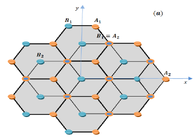
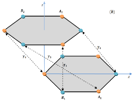
Figure 1: Lattice structure of bilayer graphene with ($A$,$B$) atoms within the same layer

We consider bilayer graphene in the presence of a perpendicular static electric and magnetic fields. The charge carriers are scattered by a single barrier potential along the $x$-direction which results in three different scattering regions denoted by ${\sf I},{\sf II}$ and ${\sf III}$. Based on the tight binding approach we can write the Hamiltonian of the system in the long wavelength limit [21, 22], and the associated eigenstates $\psi(x,y)$ as follows

$$H=\left(\begin{array}[]{cccc}V^{+}&v_{F}\pi^{+}&-v_{4}\pi^{+}&v_{3}\pi\\ v_{F}\pi&V^{+}&\gamma_{1}&-v_{4}\pi^{+}\\ -v_{4}\pi&\gamma_{1}&V^{-}&v_{F}\pi^{+}\\ v_{3}\pi^{+}&-v_{4}\pi&v_{F}\pi&V^{-}\\ \end{array}\right),\qquad\psi(x,y)=\left(\begin{array}[]{cccc}\psi_{A_{1}}(x,y)\\ \psi_{B_{1}}(x,y)\\ \psi_{A_{2}}(x,y)\\ \psi_{B_{2}}(x,y)\\ \end{array}\right).$$ (1)

Here $\pi=p_{x}+ip_{y}$, $p_{j}=-i\hbar\nabla_{j}+eA_{j}(x,y)$ is the j-th component of in-plane momentum relative to the Dirac point, $v_{F}=\frac{3a}{2}\frac{\gamma_{0}}{\hbar}=10^{6}m/s$ is the Fermi velocity for electrons in each graphene layer, $V^{+}$ and $V^{-}$ are the potentials on the first and second layer, and $v_{3,4}=\frac{v_{F}\gamma_{3,4}}{\gamma_{0}}$ are the effective velocities. We first choose the following potential barrier in each region as shown in Figure 2, the system is infinite along the $y$-axis

$$V^{\tau}=\left\{\begin{array}[]{lll}{0}&\mbox{if}&{x<d_{1}}\\ {V+\tau\delta}&\mbox{if}&{d_{1}<x<d_{2}}\\ {0}&\mbox{if}&{x>d_{2}}\end{array}\right.$$ (2)

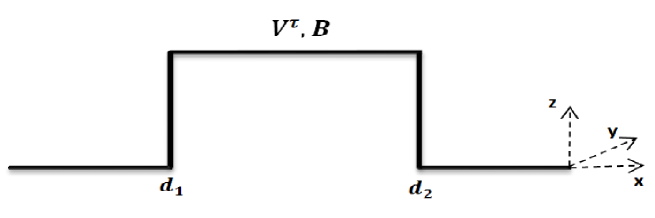
Figure 2: Schematic diagram for the bilayer graphene barrier.

where $\tau=+1$ for the first layer and $\tau=-1$ for the second layer so that $2\delta$ represents the strength of the interlayer electrostatic potential difference and $V$ is the barrier potential strength. Choosing the magnetic field to be perpendicular to the graphene layers, along the $z$-direction and defined by $B(x,y)=B\Theta\left[(d_{1}-x)(d_{2}-x)\right]$ (with constant $B$), where $\Theta$ is the Heaviside step function. In the Landau gauge, the corresponding vector potential $A(x,y)=(0,A_{y}(x))$ giving rise to the above uniform magnetic field takes the form

$$A_{y}(x)=\frac{\hbar}{el_{B}^{2}}\left\{\begin{array}[]{lll}{d_{1}}&\mbox{if}&{x<d_{1}}\\ {x}&\mbox{if}&{d_{1}<x<d_{2}}\\ {d_{2}}&\mbox{if}&{x>d_{2}}\\ \end{array}\right.$$ (3)

where $l_{B}=\sqrt{\hbar/eB}$ is the magnetic length and $e$ is the electronic charge. Since $[H,p_{y}]=0$ requires conservation of momentum along the $y$-direction then we can solve the eigenvalue problem using separation of variables and write the eigenspinors as a plane wave in the $y$-direction so that our wave function reads

$$\psi(x,y)=e^{ik_{y}y}\psi(x,k_{y})$$ (4)

At low energies the effect of the parameters v3 and v4 in our original Hamiltonian are negligible on the transmission coefficient [16]. Therefore, our Hamiltonian (1) and its associated wavefunction become

$$H=\left(\begin{array}[]{cccc}V^{+}&v_{F}\pi^{+}&0&0\\ v_{F}\pi&V^{+}&\gamma_{1}&0\\ 0&\gamma_{1}&V^{-}&v_{F}\pi^{+}\\ 0&0&v_{F}\pi&V^{-}\\ \end{array}\right),\qquad\psi(x,y)=\left(\begin{array}[]{cccc}\psi_{A_{1}}(x,y)\\ \psi_{B_{1}}(x,y)\\ \psi_{A_{2}}(x,y)\\ \psi_{B_{2}}(x,y)\\ \end{array}\right).$$ (5)

In the Appendix we solve explicitly our eigenvalue equations and obtain the following expression for the energy

$$E = V+\frac{1}{\sqrt{6}}\left[\pm\left[\mu^{\frac{1}{3}}+(A^{2}+3C)\mu^{\frac{-1}{3}}+2A\right]^{\frac{1}{2}}\right.$$

$$\left.\pm\left[-6B\sqrt{6}\left(\mu^{\frac{1}{3}}+(A^{2}+3C)\mu^{-\frac{1}{3}}+2A\right)^{-\frac{1}{2}}-\left(\mu^{\frac{1}{3}}+(A^{2}+3C)\mu^{-\frac{1}{3}}-4A\right)\right]^{\frac{1}{2}}\right]$$

where we defined the quantities

$${\mu=-A^{3}+27B^{2}+9AC+3\sqrt{3}\left[-\left(A^{2}+3C\right)^{3}+\left(-A^{3}+27B^{2}+9AC\right)^{2}\right]^{\frac{1}{2}}}$$ (7)

$${A=\delta^{2}+(2n+1)\vartheta_{0}^{2}+\frac{\gamma_{1}^{2}}{2}}$$ (8)

$${B=\vartheta_{0}^{2}\delta}$$ (9)

$${C=\left((2n+1)\vartheta_{0}^{2}-\delta^{2}\right)^{2}-\vartheta_{0}^{4}+\gamma_{1}^{2}\delta^{2}}$$ (10)

with $\vartheta_{0}=\frac{\hbar v_{F}}{l_{B}}$ is the energy scale and $n$ is an integer number. To exhibit the main features of our four energy bands (2), we plot the energy in terms of the magnetic field $B$ in Figure 3. For $\delta=0$ and the Landau levels $(n=1,2,3)$, we observe in Figure 3(a) that for the first and second layers we have $E=V$ and $E=V\pm\gamma$, respectively, which correspond to $B=0$. The situation changes in Figure 3(b) when we consider $\delta\neq 0$ the energy then becomes $E=V\pm\delta$ for $B=0$ and therefore $\Delta E=2\delta$ represents the gap in the energy spectrum. While in both cases, the energy increases/decreases as long as $B$ and the Landau levels increases inside the barrier.

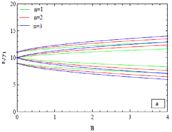
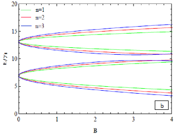
Figure 3: The four energy eigenvalues inside the barrier region as a function of the magnetic field $B$, with $V=10~{}\gamma_{1}$. (a) and (b) for $\delta=0~{}\gamma_{1}$ and $\delta=3~{}\gamma_{1}$, respectively.

For $\delta=0$, that is in the absence of electric field, (2) reduces to [23]

$$E=V\pm\sqrt{(2n+1)\vartheta_{0}^{2}+\frac{\gamma_{1}^{2}}{2}\pm\sqrt{(2n+1)\vartheta_{0}^{2}\gamma_{1}^{2}+\vartheta_{0}^{4}+\frac{\gamma_{1}^{4}}{4}}}.$$ (11)

These energy eigenvalues will reduce to the case of a single graphene layer where $\gamma_{1}\longrightarrow 0$, to give $E=V\pm\vartheta_{0}\sqrt{2n+1\pm 1}$.

Outside the barrier region, the energy expression can be defined as follows

$$\epsilon=\pm\sqrt{k_{1,2}^{2}+\frac{\Gamma_{1}^{2}}{2}\pm\sqrt{\Gamma_{1}^{2}k_{1,2}^{2}+\frac{\Gamma_{1}^{4}}{4}}}$$ (12)

where $\epsilon=E/\hbar v_{F}$, $\Gamma_{1}=\gamma_{1}/\hbar v_{F}$ and

$$k_{1,2}=\sqrt{\left(\alpha_{1,2}^{\pm}\right)^{2}+\left(k_{y}+\frac{d_{1,2}}{{l_{B}}^{2}}\right)^{2}}$$ (13)

$\alpha_{1}^{\pm}$ being the wave vector of the propagating wave in the first region where there are two right-going (incident) propagating modes and two left-going (reflected) propagating modes. $\alpha_{2}^{\pm}$ is the wave vector of the propagating wave in the third region with two right-going (transmission) propagating modes. We plot the energy (12) in Figure 4 to show its behavior in each region which depends on the propagating modes. It is clear that the behavior is different in region ${\sf I}$ (red line) and region ${\sf III}$ (dashed line), as compared to the cases of a simple and double barrier in the absence of magnetic field [16, 17].

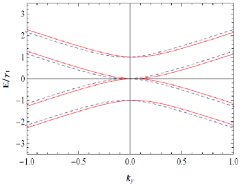
Figure 4: The four energy eigenvalues outside the barrier region as a function of the wave vector $k_{y}$ along the $y$-direction for $l_{B}=13.5~{}nm$ and $d_{2}=-d_{1}=7.5~{}nm$, where red (dashed) line correspond to region ${\sf I}$ (region ${\sf III}$).

Next we will calculate the transmission and reflection coefficients of electrons across the potential barrier in our bilayer graphene system.

3 Transmission probability and conductance

The transmission and reflection coefficients are obtained by imposing the continuity of the wave function at each potential interface. The wave function given in the Appendix can be used in each region denoted by the integer $j$, which can then be rewritten in a matrix notation as

$$\psi_{j}=G_{j}\cdot M_{j}\cdot A_{j}$$ (14)

where the index $j$ denotes each potential region, $j={\sf I}$ for the incident region ( $x<d_{1}$ ), $j={\sf II}$ for the potential barrier region ( $d_{1}<x<d_{2}$ ) and $j={\sf III}$ for the transmission region ( $x>d_{2}$ ). Outside the barrier region, $A_{\sf I}^{\pm}$ and $A_{\sf III}^{\pm}$ are defined by

$$A_{\sf I}^{\pm}=\left(\begin{array}[]{c}\delta_{\pm,1}\\ r_{+}^{\pm}\\ \delta_{\pm,-1}\\ r_{-}^{\pm}\\ \end{array}\right),\qquad A_{\sf III}^{\pm}=\left(\begin{array}[]{c}t_{+}^{\pm}\\ 0\\ t_{-}^{\pm}\\ 0\\ \end{array}\right)$$ (15)

$\pm$ indicates the wave vector $\alpha_{1,2}^{\pm}$ as defined in the Appendix and $\delta_{\pm,1}$ is the Kronecker delta function, $G_{\sf I,III}$ and $M_{\sf I,III}$ are defined by

$$G_{\sf I,III}=\left(\begin{array}[]{cccc}f_{1,2}^{++}&f_{1,2}^{+-}&f_{1,2}^{-+}&f_{1,2}^{--}\\ 1&1&1&1\\ -1&-1&1&1\\ -g_{1,2}^{++}&-g_{1,2}^{+-}&g_{1,2}^{-+}&g_{1,2}^{--}\\ \end{array}\right)$$ (16)

and

$$M_{\sf I,III}=\left(\begin{array}[]{cccc}e^{i\alpha_{1,2}^{+}x}&0&0&0\\ 0&e^{-i\alpha_{1,2}^{+}x}&0&0\\ 0&0&e^{i\alpha_{1,2}^{-}x}&0\\ 0&0&0&e^{-i\alpha_{1,2}^{+}x}\\ \end{array}\right).$$ (17)

Inside the barrier region, we have $A_{\sf II}=(c_{+},c_{-},d_{+},d_{-})^{T}$ and $G_{\sf II}$

$$G_{\sf II}=\left(\begin{array}[]{cccc}\eta_{-}\lambda_{+}\chi_{-1}^{++}&\eta_{-}^{*}\lambda_{+}\chi_{-1}^{+-}&\eta_{-}\lambda_{-}\chi_{-1}^{-+}&\eta_{-}^{*}\lambda_{-}\chi_{-1}^{--}\\ \chi_{0}^{++}&\chi_{0}^{+-}&\chi_{0}^{-+}&\chi_{0}^{--}\\ \zeta^{+}\chi_{0}^{++}&\zeta^{+}\chi_{0}^{+-}&\zeta^{-}\chi_{0}^{-+}&\zeta^{-}\chi_{0}^{--}\\ \eta_{+}^{*}\zeta^{+}\chi_{1}^{++}&\eta_{+}\zeta^{+}\chi_{1}^{+-}&\eta_{+}^{*}\zeta^{-}\chi_{1}^{-+}&\eta_{+}\zeta^{-}\chi_{1}^{--}\end{array}\right)$$ (18)

where $\chi_{l}^{\pm\pm}=D[\lambda_{\pm}+l,\pm Z]$ and $M_{\sf II}=\mathbb{I}_{4}$.

The continuity boundary conditions at $x=d_{1}$ and $x=d_{2}$ can be written in a matrix notation as

$${G_{\sf I}\cdot M_{\sf I}(x=d_{1})\cdot A_{\sf I}^{\pm}=G_{\sf II}(x=d_{1})\cdot M_{\sf II}\cdot A_{\sf II}}$$ (19)

$${G_{\sf III}\cdot M_{\sf III}(x=d_{2})\cdot A_{\sf III}^{\pm}=G_{\sf II}(x=d_{2})\cdot M_{\sf II}\cdot A_{\sf II}}.$$ (20)

Using the transfer matrix method we can connect $A_{\sf I}^{\pm}$ with $A_{\sf III}^{\pm}$ through the matrix $N$

$$N=M_{\sf I}^{-1}(x=d_{1})\cdot G_{\sf I}^{-1}\cdot G_{\sf II}(x=d_{1})\cdot G_{sfII}^{-1}(x=d_{2})\cdot G_{\sf III}\cdot M_{\sf III}(x=d_{2})$$ (21)

with the help of the relation $A_{\sf I}^{\pm}=NA_{\sf III}^{\pm}$, the transport coefficients can then be derived from

$$\left(\begin{array}[]{c}t_{+}^{\pm}\\ r_{+}^{\pm}\\ t_{-}^{\pm}\\ r_{-}^{\pm}\\ \end{array}\right)=\left(\begin{array}[]{cccc}N_{11}&0&N_{13}&0\\ N_{21}&-1&N_{23}&0\\ N_{31}&0&N_{33}&0\\ N_{41}&0&N_{43}&-1\\ \end{array}\right)^{-1}\cdot\left(\begin{array}[]{c}\delta_{\pm,1}\\ 0\\ \delta_{\pm,-1}\\ 0\\ \end{array}\right)$$ (22)

where $N_{ij}$ are the matrix elements of the matrix $N$. Then the transmission and reflection coefficients can be obtained as

$${t_{+}^{\pm}=\frac{N_{13}\delta_{\pm,-1}-N_{33}\delta_{\pm,1}}{N_{13}N_{31}-N_{33}N_{11}}}$$ (23)

$${t_{-}^{\pm}=\frac{-N_{11}\delta_{\pm,-1}+N_{31}\delta_{\pm,1}}{N_{31}N_{13}-N_{11}N_{33}}}$$ (24)

$${r_{+}^{\pm}=N_{21}t_{+}^{\pm}+N_{23}t_{-}^{\pm}}$$ (25)

$${r_{-}^{\pm}=N_{41}t_{+}^{\pm}+N_{43}t_{-}^{\pm}}.$$ (26)

On the other hand, the transmission and refection probabilities can be obtained using the current density corresponding to our system. This is

$$\vec{J}=\pm i\psi^{\dagger}(x,k_{y})\vec{\sigma}\psi(x,k_{y})$$ (27)

where $J$ defines the electric current density for our system. Computing explicitly equation (27) gives for the incident, reflected and transmitted current densities

$${J_{x}^{\sf inc}=\pm 4i\frac{\alpha_{1}^{\pm}}{\epsilon}}$$ (28)

$${J_{x}^{\sf ref}=\mp 4i\frac{\alpha_{1}^{\pm}}{\epsilon}(r_{\pm}^{\pm})^{*}r_{\pm}^{\pm}}$$ (29)

$${J_{x}^{\sf tra}=\pm 4i\frac{\alpha_{2}^{\pm}}{\epsilon}(t_{\pm}^{\pm})^{*}t_{\pm}^{\pm}}$$ (30)

which gives rise to the probabilities

$${T_{\pm}^{\pm}=\frac{\mid{J_{x}^{\sf tra}\mid}}{\mid{J_{x}^{\sf inc}\mid}}=\frac{\alpha_{2}^{\pm}}{\alpha_{1}^{\pm}}\mid t_{\pm}^{\pm}\mid^{2}}$$ (31)

$${R_{\pm}^{\pm}=\frac{\mid{J_{x}^{\sf ref}\mid}}{\mid{J_{x}^{\sf inc}\mid}}=\frac{\alpha_{1}^{\pm}}{\alpha_{1}^{\pm}}\mid r_{\pm}^{\pm}\mid^{2}}.$$ (32)

Therefore, we ended up with four transport channels for transmissions and reflections probabilities because we have four bands. Since electrons can be scattered into four propagation modes then we need to take into account the change in their wave velocities. The conductance of our system can be expressed in terms of the transmission probability using the famous Landauer-B$\ddot{u}$ttiker formula [24]

$$G=G_{0}\frac{L_{y}}{2\pi}\int_{-\infty}^{\infty}dk_{y}\sum_{\pm,\pm}T_{\pm}^{\pm}\left(E,k_{y}\right)$$ (33)

where $G_{0}=Ne^{2}/(2\pi\hbar)\approx 3.87\times 10^{-5}N\Omega^{-1}$, $N$ is the number of transverse channels and $L_{y}$ is the width of the sample in the $y$-direction.

We will investigate numerically two interesting cases depending on the value of the incident energies, $E$, as compared with the interlayer coupling parameter $\gamma_{1}$. The two band tunneling leads to one transmission and one reflection channel, takes place at energies less than the interlayer coupling ($E<\gamma_{1}$) since we have juste one mode of propagation $\alpha^{+}$. On the other hand, for energies higher than the interlayer coupling parameter $\gamma_{1}$ ($E>\gamma_{1}$), the four band tunneling takes place and gives rise to four transmission and four reflection channels. We denote them as $T_{+}^{+}$ and $T_{-}^{-}$ for scattering from the $\alpha^{+}$ and $\alpha^{-}$, respectively. Therefore, we have two transmission channels ($T_{-}^{+}$ and $T_{+}^{-}$) of electrons moving in opposite direction (from $\alpha^{+}$ to $\alpha^{-}$ and $\alpha^{-}$ to $\alpha^{+}$). In the next sections we will study each of these regimes separately. For numerical convenience we fix $\vartheta_{0}/\gamma_{1}=1.64/l_{B}$ in the rest of the paper.

4 Two Band Tunneling

To allow for a suitable interpretation of our main results in the low energy regime ($E<\gamma_{1}$), we compute numerically the transmission probability under various conditions. First we plot the transmission probability at normal incidence ($k_{y}l_{B}=-d_{1}/l_{B}=0$) as a function of the Fermi energy $E$, for $V=0.3~{}\gamma_{1}$ and three different values of the barrier width $d=25~{}nm$ (red line), $d=30~{}nm$ (blue line), and $d=40~{}nm$ (green line), see Figure 5. Note that Figures (a)/(b) have been produced for $\delta=0.0~{}\gamma_{1}$/$\delta=0.1~{}\gamma_{1}$ and $l_{B}=13.5~{}nm$ while Figures (c)/(d) were done for $\delta=0.0~{}\gamma_{1}$/$\delta=0.1~{}\gamma_{1}$ and $l_{B}=18.5~{}nm$. We note that in Figure 5(a), when the energy is less than the height of the barrier potential, i.e $E<V$, we have zero transmission, while, when the energy is more then the height of the barrier Dirac fermions exhibit transmission resonances. As usual the transmission probability is slightly displaced to the left as we increase the width of the barrier. Figure 5(b) shows the transmission for the same parameters 5(a) but with $\delta=0.1~{}\gamma_{1}$. It is clear that the transmission probability is affected by the transmission gap $\Delta E=2~{}\delta$. To understand more accurately our system and study the effect of the magnetic length parameters $l_{B}$ on the transmission as function of the Fermi energy $E$ for different values of the magnetic length parameters. Using the barrier parameters used in Figure 5(a) but with $l_{B}=18.5~{}nm$, see show in Figure 5(c) and 5(d) we show the transmission for zero gap $\delta=0.0~{}\gamma_{1}$ and finite gap $\delta=0.1~{}\gamma_{1}$, respectively. We can clearly see that as we increase $l_{B}$ the transmission resonances increase in number while the transmission probability exhibit a translation to left as we increase the barrier width.

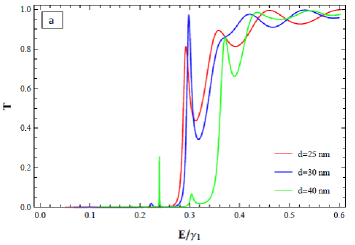
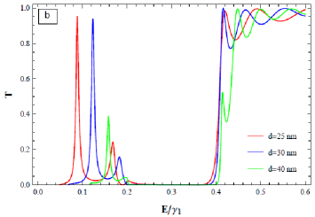
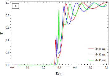
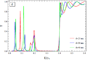
Figure 5: Plot of transmission probability as a function of the Fermi energy $E$ at normal incidence, for $V=0.3~{}\gamma_{1}$. (a)/(b) for $\delta=0.0~{}\gamma_{1}$/$\delta=0.1~{}\gamma_{1}$ and $l_{B}=13.5~{}nm$ . (c)/(d) for $\delta=0.0~{}\gamma_{1}$/$\delta=0.1~{}\gamma_{1}$ and $l_{B}=18.5~{}nm$.

Figures 6(a) and 6(c) show a comparison of the density plots for the transmission probability at normal incidence $k_{y}l_{B}=-d_{1}/l_{B}=0$ and non-normal incidence $k_{y}l_{B}\neq-d_{1}/l_{B}$ ($d_{1}=0~{}nm$ and $k_{y}=0.05~{}nm^{-1}$), as a function of the barrier width $d$ and energy $E$, respectively, for $\delta=0.0~{}\gamma_{1}$ and $V=0.3~{}\gamma_{1}$ in both cases. In Figures 6(b) and 6(d) we used the same parameters as in 6(a) and 6(c), respectively, but with $\delta=0.1~{}\gamma_{1}$. One notices that, at normal incidence and for $\delta=0.0~{}\gamma_{1}$ the transmission probability shown in Figure 6(a) is zero and there are no resonances within a range of energy less than the height of the barrier potential, i.e $E<V$. On the other hand resonances are present at non-normal incidence as shown in Figure 6(c). When the energy is more than the height of the barrier potential the transmission exhibits resonances. As observed in Figures 6(b) and 6(d) the transmission probability is related to the transmission gap $\Delta E=2~{}\delta$ and remains invariant for $E>V+\delta$. We also observe that the number of resonances in the transmission as shown in Figures 6(b) and 6(d) decreases for $E<V-\delta$.

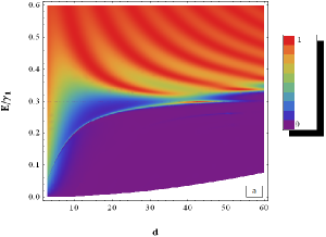
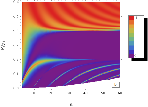
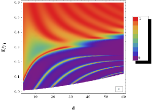
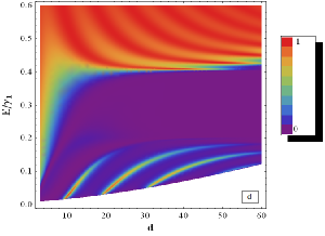
Figure 6: Density plot of transmission probability as a function of the barrier width $d$ and energy $E$, for $V=0.3~{}\gamma_{1}$ and $l_{B}=18.5~{}nm$. (a)/(b) for $\delta=0.0~{}\gamma_{1}$/$\delta=0.1~{}\gamma_{1}$ at normal incidence $k_{y}l_{B}=-d_{1}/l_{B}=0$. (c)/(d) for $\delta=0.0~{}\gamma_{1}$/$\delta=0.1~{}\gamma_{1}$ at non-normal incidence $k_{y}l_{B}\neq-d_{1}/l_{B}$($d_{1}=0~{}nm$ and $ky=0.05~{}nm^{-1}$).

In Figure 7, we show the density plot of the transmission probability as a function of the transverse wave vector $k_{y}$ and energy $E$ for two values of the barrier width : $d=30~{}nm$ ($d_{2}=-d_{1}=15~{}nm$) in Figures 7(a) and 7(b), and $d=40~{}nm$ ($d_{2}=-d_{1}=20~{}nm$) in Figures 7(c) and 7(d). To see the effect of the barrier width $d$ on the transmission probability at non-normal incidence we show in Figure 7(a) that when we increase $d$ a new peak of resonance appear within the range of energy less than the height of the barrier potential, i.e $E<V$.The number of these resonance peaks depends on the width of the well between the barriers. At nearly normal incidence $\mid k_{y}\mid\approx-\mid\frac{d_{1}}{l_{B}^{2}}\mid\approx 0.04~{}nm^{-1}$ in Figure 7(a), and $\mid k_{y}\mid\approx-\mid\frac{d_{1}}{l_{B}^{2}}\mid\approx 0.06~{}nm^{-1}$ in Figure 7(c) we have zero transmission when the energy is less than the height of the barrier potential. On the other hand, for energy more than the height of the barrier the Dirac fermions exhibit transmission resonances as seen in Figures 7(a) and 7(b), the number of transmission resonances increase when we increase the barrier width $d$ as shown in Figures 7(c) and 7(d), respectively. We remark from Figures 7(b) and 7(d) that the transmission probability is correlated to the transmission gap $\Delta E=2~{}\delta$.

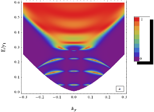
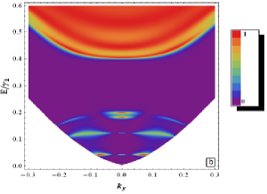
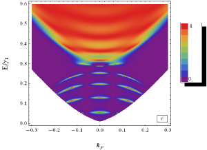
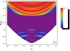
Figure 7: Density plot of transmission probability as a function of the transverse wave vector $k_{y}$ and energy $E$, for $V=0.3~{}\gamma_{1}$ and $l_{B}=18.5~{}nm$. (a)/(b) for $\delta=0.0~{}\gamma_{1}$/$\delta=0.1~{}\gamma_{1}$, respectively, and $d=30~{}nm$. (c)/(d) for $\delta=0.0~{}\gamma_{1}$/$\delta=0.1~{}\gamma_{1}$, respectively, and $d=40~{}nm$.

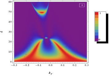
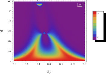
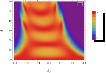
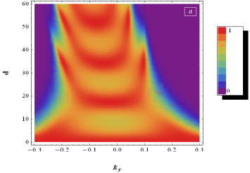
Figure 8: Density plot of transmission probability as a function of the transverse wave vector $k_{y}$ and the barrier width $d$, for $V=0.3~{}\gamma_{1}$ and $l_{B}=18.5~{}nm$. (a)/(b) for $\delta=0.0~{}\gamma_{1}$/$\delta=0.02~{}\gamma_{1}$ and $E=\frac{9}{10}~{}V$. (c)/(d) for $\delta=0.0~{}\gamma_{1}$/$\delta=0.05~{}\gamma_{1}$ and $E=\frac{13}{10}~{}V$.

In Figure 8 we show the density plot of transmission probability as function of the transfer wave vector $k_{y}$ and the barrier width $d$, for $V=0.3~{}\gamma_{1}$ and $l_{B}=18.5~{}nm$. In Figures 8(a) and 8(b) we fix the energy at $E=\frac{9}{10}~{}V$, for two different values of the interlayer potential $\delta=0.0~{}\gamma_{1}$ and $\delta=0.02~{}\gamma_{1}$. In Figures 8(c) and 8(d) we fix the energy at $E=\frac{13}{10}~{}V$ again for two different values of the interlayer electrostatic potential $\delta=0.0~{}\gamma_{1}$ and $\delta=0.05~{}\gamma_{1}$. For $\delta=0.0~{}\gamma_{1}$ and for energy less than the height of the potential barrier, $E<V$, we have full transmission for a wide range of $k_{y}$ values. By increasing the width $d$, we create one resonance peak as depicted in Figure 8(a). However, the total transmission probability decreases for $\delta=0.02~{}\gamma_{1}$ as shown in Figure 8(b). In Figure 8(c) most of the resonances disappear while oscillations take over in the transmission. The number of oscillations decrease in presence of the interlayer electrostatic potential as reflected in Figure 8(d).

5 Four band tunneling

Once we allow for higher energies, $E>\gamma_{1}$, we will have four transmission and four reflection channels resulting in what we call the four band tunneling.

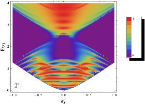
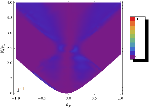
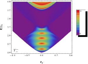
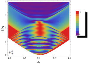
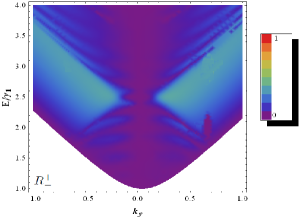
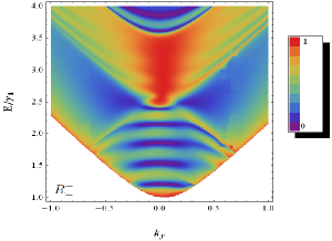
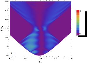
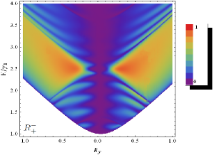
Figure 9: Density plot of transmission and reflection coefficients as a function of the transverse wave vector $k_{y}$ and energy $E$ with $V=2.5~{}\gamma_{1}$, $\delta=0.0~{}\gamma_{1}$, $l_{B}=13.5~{}nm$ , and $d_{2}=-d_{1}=7.5~{}nm$ .

In Figure 9 we show the transmission and reflection probabilities associated with different channels, as a function of the transverse wave vector $k_{y}$ and the incident energy $E$, we used $V=2.5~{}\gamma_{1}$, $\delta=0.0~{}\gamma_{1}$, $l_{B}=13.5~{}nm$, and $d_{2}=-d_{1}=7.5~{}nm$. For energies less than $V-\gamma_{1}$ the Dirac fermions exhibit transmission resonances in $T_{+}^{+}$ in which the electrons propagate via $\alpha^{+}$ mode inside the barriers. For $V-\gamma_{1}<E<V$, there are no available $\alpha^{+}$ states and the transmission is suppressed in this region. For nearly normal incidence, $k_{y}\approx-\frac{d_{2}}{l_{B}^{2}}\approx-0.04~{}nm^{-1}$ for $T_{-}^{+}$ and $k_{y}\approx-\frac{d_{1}}{l_{B}^{2}}\approx 0.04~{}nm^{-1}$ for $T_{+}^{-}$, the cloak effect [25] occurs in the energy region $V-\gamma_{1}<E<V$, where the two modes $\alpha^{+}$ outside and inside barrier regions are decoupled and therefore no scattering occur between them [16] in the $T_{-}^{+}$ and $T_{+}^{-}$ channels. While for non-normal incidence the two modes $\alpha^{+}$ outside and inside barrier region are coupled, so that the transmission $T_{-}^{+}$ and $T_{+}^{-}$ channels in the same energy region are non-zero. The transmission probabilities $T_{-}^{+}$ and $T_{+}^{-}$ are different ( $T_{-}^{+}\neq T_{+}^{-}$), which introduces an asymmetry for a single barrier due to the presence of the magnetic field. In addition, the reflection coefficients $R_{-}^{+}$ and $R_{+}^{-}$ are different ($R_{-}^{+}\neq R_{+}^{-}$) and do not have the same number of resonances and anti-resonance, these observations were absent in the case of single and double barrier in the absence of magnetic field [16, 17]. For $T_{-}^{-}$ and $R_{-}^{-}$ the electrons propagate via $\alpha^{-}$ mode for $E<V$ and $E>V+\gamma_{1}$, which is blocked inside the barrier for $V<E<V+\gamma_{1}$ so that the transmission is suppressed in this region and this is equivalent to the cloak effect [16, 17].

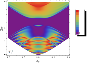
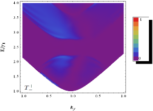
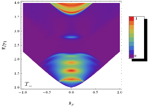
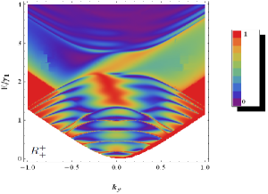
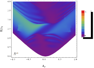
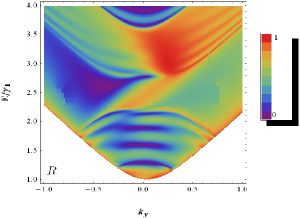
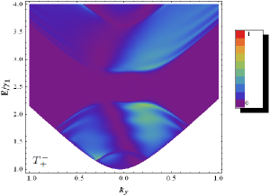
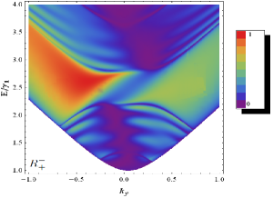
Figure 10: Density plot of transmission and reflection coefficients as a function of the transverse wave vector $k_{y}$ and energy $E$ for $V=2.5~{}\gamma_{1}$, $\delta=0.3~{}\gamma_{1}$, $l_{B}=13.5~{}nm$, and $d_{2}=-d_{1}=7.5~{}nm$.

To probe the effect of the interlayer electrostatic potential $\delta$, we investigate the density plot of the transmission probability as function of the transfer wave vector $k_{y}$ and energy $E$, using the same parameters as in Figure 8 but for $\delta=0.3~{}\gamma_{1}$ in Figure 10. We note that the transmission probability in the energy region $V-\delta<E<V+\delta$ is correlated to the transmission gap and shows a suppression due to cloak effect, as it was the case for the single barrier [16].

6 Conductance

In Figure 11 we show the conductance through a single barrier structure in the presence of a magnetic field as a function of the energy $E$ for $V=2.5~{}\gamma_{1}$, $d_{2}=-d_{1}=7.5~{}nm$ for $l_{B}=13.5~{}nm$ (solid) and $l_{B}=18.5~{}nm$ (dotted). For energies smaller than the barrier s height, the peaks in the conductance through a single barrier in the presence of a magnetic field, which are magnified in the inset of Figure 11(a), have shoulders due to the presence of resonances in the transmission probability $T_{+}^{+}$ in the region $0<E<V$ and that of $T_{+}^{-}$, $T_{-}^{+}$, and $T_{-}^{-}$ in the region $\gamma_{1}<E<V$ as depicted in Figure 9. The resonance peaks of the conductance resulting from propagation via $\alpha^{+}$ modes in the region $E<V-\gamma_{1}$, appear as shoulders of on other peaks [16]. Additional resonance peaks appear due to propagation via $\alpha^{-}$ modes inside the barrier for energy larger than $\gamma_{1}$, $E>\gamma_{1}$. We should mention the inequality of the two channels $T_{-}^{+}\neq T_{+}^{-}$ due to the asymmetry in the presence of the magnetic field. For $V<E<V+\gamma_{1}$ the contribution of $T_{-}^{-}$ is zero due to the cloak effect [16, 17]. To see the effect of the interlayer electrostatic potential, we plot the conductance as function of the energy $E$ in Figures 11(b) and notice that the conductance in the energy region $\Delta E=2\delta$ is correlated to the transmission gap.

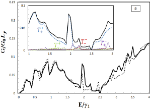
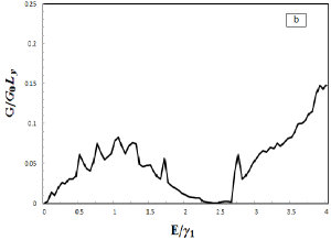
Figure 11: Conductance through the single barrier structure in the presence of a magnetic field as a function of energy for $V=2.5~{}\gamma_{1}$ and $d_{2}=-d_{1}=7.5$ nm. (a) for $\delta=0.0~{}\gamma_{1}$, $l_{B}=13.5~{}nm$ (solid) and $l_{B}=18.5~{}nm$ (dotted). (b) for $\delta=0.3~{}\gamma_{1}$ and $l_{B}=13.5~{}nm$ (solid).

7 Conclusion

In the present work we computed the transmission probability through rectangular potential barriers and p-n junctions in the presence of both electric and magnetic static fields in bilayer graphene. The tight binding model that describes our system leads to the formation of four bands in the associated energy spectrum. The richness of the energy spectrum allows for two propagation modes whose energy scale is set by the interlayer coupling $\gamma_{1}$. For energies higher than the interlayer coupling $\gamma_{1}$, $E~{}>~{}\gamma_{1}$, two propagation modes are available for transport, and four possible ways for transmission and reflection coefficients, while, when the energy is less than $\gamma_{1}$ the Dirac fermions have only one mode of propagation available to them. The resulting conductance incorporates these new transport channels which manifest themselves by the presence of more resonances and larger values of the conductance at high energies. The presence of an externally controlled electrostatic potential $\delta$ created an asymmetry between the on-site energies in the two layers which then resulted in a tunable energy gap between the conduction and valence energy bands. Hence we studied the effect of the interlayer electrostatic potential $\delta$ and the various barrier geometry parameters on the transmission probability.

Appendix: Wavefunction of our system

Hamiltonian (5) was used in the Schrodinger equation $H\psi(x,y)=E\psi(x,y)$ which can then be written as four linear differential equations of the from

$${-i\hbar v_{F}\frac{\sqrt{2}}{l_{B}}a\psi_{B_{1}}(x,k_{y})=(E-V-\delta)\psi_{A_{1}}(x,k_{y})\qquad\qquad\quad\quad\quad~{}~{}}$$ (A-1a)

$${i\hbar v_{F}\frac{\sqrt{2}}{l_{B}}a^{+}\psi_{A_{1}}(x,k_{y})=(E-V-\delta)\psi_{B_{1}}(x,k_{y})-\gamma_{1}\psi_{A_{2}}(x,k_{y})\quad}$$ (A-1b)

$${\quad\quad-i\hbar v_{F}\frac{\sqrt{2}}{l_{B}}a\psi_{B_{2}}(x,k_{y})=(E-V+\delta)\psi_{A_{2}}(x,k_{y})-\gamma_{1}\psi_{B_{1}}(x,k_{y})~{}~{}~{}}$$ (A-1c)

$${i\hbar v_{F}\frac{\sqrt{2}}{l_{B}}a^{+}\psi_{A_{2}}(x,k_{y})=(E-V+\delta)\psi_{B_{2}}(x,k_{y})\qquad\qquad\qquad\quad~{}}$$ (A-1d)

where $a=\frac{l_{B}}{\sqrt{2}}\left(\partial_{x}+k_{y}+\frac{e}{\hbar}A_{y}(x)\right)$ and $a^{+}=\frac{l_{B}}{\sqrt{2}}\left(-\partial_{x}+k_{y}+\frac{e}{\hbar}A_{y}(x)\right)$ are the annihilation and creation operators. We find the expression of $\psi_{A_{1}}(x,k_{y})$ in (A-1a) and $\psi_{B_{2}}(x,k_{y})$ in (A-1d), and replace both $\psi_{A_{1}}(x,k_{y})$ and $\psi_{B_{2}}(x,k_{y})$ in (A-1b) and (A-1c), respectively. This gives

$${\left(2\vartheta_{0}^{2}a^{+}a-(E-V-\delta)^{2}\right)\psi_{B_{1}}(x,k_{y})=-\gamma_{1}(E-V-\delta)\psi_{A_{2}}(x,k_{y})~{}~{}}$$ (A-2a)

$${\left(2\vartheta_{0}^{2}aa^{+}-(E-V+\delta)^{2}\right)\psi_{A_{2}}(x,k_{y})=-\gamma_{1}(E-V+\delta)\psi_{B_{1}}(x,k_{y})~{}~{}}$$ (A-2b)

where $\vartheta_{0}=\frac{\hbar v_{F}}{l_{B}}$ is the energy scale. Combining the above equations we obtain

$$\left[2\vartheta_{0}^{2}aa^{+}-(E-V+\delta)^{2}\right]\left[2\vartheta_{0}^{2}a^{+}a-(E-V-\delta)^{2}\right]\psi_{B_{1}}(x,k_{y})=\gamma_{1}^{2}((E-V)^{2}-\delta^{2})\psi_{B_{1}}(x,k_{y})$$ (A-3)

Solving the eigenvalue equation we end up with the eigenspinors outside $(x<d_{1},x>d_{2})$ and inside $(d_{1}<x<d_{2})$ the barrier regions which result in the following two situations:

a) Inside the barrier region

In region ${\sf II}$ ($d_{1}<x<d_{2})$, the vector potential $A_{y}(x)$ is given by $\frac{\hbar}{el_{B}^{2}}x$ which can then expressed in terms of annihilation and creation operators ($a$ and $a^{+}$). Using the envelope function $\psi_{B_{1}}(x,k_{y})\equiv\psi_{B_{1}}(X)$ that depend on a combination of the variables, $X=\frac{x}{l_{B}}+k_{y}l_{B}$, we can rewrite $a$ and $a^{+}$ as follows $a=\frac{1}{\sqrt{2}}\left(\partial_{X}+X\right)$ and $a^{+}=\frac{1}{\sqrt{2}}\left(-\partial_{X}+X\right)$. Our differential equation becomes

$$\left[-\partial_{X}^{2}+X^{2}-1-2\lambda_{+}\right]\left[-\partial_{X}^{2}+X^{2}-1-2\lambda_{-}\right]\psi_{B_{1}}(X)=0$$ (A-4)

where

$$\lambda_{\pm}=-\frac{1}{2}+\frac{(E-V)^{2}+\delta^{2}}{2\vartheta_{0}^{2}}\pm\frac{\sqrt{(\vartheta_{0}^{2}-2(E-V)\delta)^{2}+\gamma_{1}^{2}((E-V)^{2}-\delta^{2})}}{2\vartheta_{0}^{2}}.$$ (A-5)

Therefore, the general solution of (A-4), can be written as follows $\psi_{B_{1}}(Z)=\psi_{B_{1}}^{+}(Z)+\psi_{B_{1}}^{-}(Z)$ with

$$\begin{array}[]{ll}{\psi_{B_{1}}^{+}(Z)=c_{+}D[\lambda_{+},Z]+c_{-}D[\lambda_{+},-Z]}\\ {\psi_{B_{1}}^{-}(Z)=d_{+}D[\lambda_{-},Z]+d_{-}D[\lambda_{-},-Z]}\end{array}$$ (A-6)

and we have set $Z=\sqrt{2}X$. Using this result in equation (A-1a), gives $\psi_{A_{1}}(Z)=\psi_{A_{1}}^{+}(Z)+\psi_{A_{1}}^{-}(Z)$ with

$$\begin{array}[]{ll}{\psi_{A_{1}}^{+}(Z)=c_{+}\eta_{-}\lambda_{+}D[\lambda_{+}-1,Z]+c_{-}\eta_{-}^{*}\lambda_{+}D[\lambda_{+}-1,-Z]}\\ {\psi_{A_{1}}^{-}(Z)=d_{+}\eta_{-}\lambda_{-}D[\lambda_{-}-1,Z]+d_{-}\eta_{-}^{*}\lambda_{-}D[\lambda_{-}-1,-Z]}\end{array}$$ (A-7)

where $\eta_{\pm}=\frac{-i\sqrt{2}\vartheta_{0}}{E-V\pm\delta}$. Furthermore using both $\psi_{A_{1}}(x,k_{y})$ and $\psi_{B_{2}}(x,k_{y})$ in (A-1b) gives $\psi_{A_{2}}(Z)=\psi_{A_{2}}^{+}(Z)+\psi_{A_{2}}^{-}(Z)$ such as

$$\begin{array}[]{ll}{\psi_{A_{2}}^{+}(Z)=c_{+}\zeta^{+}D[\lambda_{+},Z]+c_{-}\zeta^{+}D[\lambda_{+},-Z]}\\ {\psi_{A_{2}}^{-}(Z)=d_{+}\zeta^{-}D[\lambda_{-},Z]+d_{-}\zeta^{-}D[\lambda_{-},-Z]}\end{array}$$ (A-8)

and $\zeta^{\pm}=\frac{E-V-\delta}{\gamma_{1}}-\frac{2\vartheta_{0}^{2}\lambda_{\pm}}{\gamma_{1}(E-V-\delta)}$ is introduced. Finally, using $\psi_{A_{2}}$ in (A-1d) gives $\psi_{B_{2}}(Z)=\psi_{B_{2}}^{+}(Z)+\psi_{B_{2}}^{-}(Z)$ with

$$\begin{array}[]{ll}{\psi_{B_{2}}^{+}(Z)=c_{+}\eta_{+}^{*}\zeta^{+}D[\lambda_{+}+1,Z]+c_{-}\eta_{+}\zeta^{+}D[\lambda_{+}+1,-Z]}\\ {\psi_{B_{2}}^{-}(Z)=d_{+}\eta_{+}^{*}\zeta^{-}D[\lambda_{-}+1,Z]+d_{-}\eta_{+}\zeta^{-}D[\lambda_{-}+1,-Z]}.\end{array}$$ (A-9)

b) Outside the barrier region

Solving the eigenvalue equation (A-3) to obtain the eigenspinor in region ${\sf I}$ ($x<d_{1}$) and in region ${\sf III}$ ($x>d_{2}$), where potential barrier $V$ and interlayer potential $\delta$ are equal to zero and the associated vector potential $A_{y}(x)$ is constant and equal to $\frac{\hbar}{el_{B}^{2}}d_{1}$ ($\frac{\hbar}{el_{B}^{2}}d_{2}$) in region ${\sf I}$ (region ${\sf III}$). We obtain the general solution in a plane-wave form $\psi_{B_{1}}(x,k_{y})=\psi_{B_{1}}^{+}(x,k_{y})+\psi_{B_{1}}^{-}(x,k_{y})$ with

$$\begin{array}[]{ll}{\psi_{B_{1}}^{+}(x,k_{y})=c_{+}e^{i\alpha_{1,2}^{+}x}+c_{-}e^{-i\alpha_{1,2}^{+}x}}\\ {\psi_{B_{1}}^{-}(x,k_{y})=d_{+}e^{i\alpha_{1,2}^{-}x}+d_{-}e^{-i\alpha_{1,2}^{-}x}}\end{array}$$ (A-10)

where $\alpha_{1,2}^{\pm}=\sqrt{(E^{2}\pm E\gamma_{1})/(\hbar v_{F})^{2}-\left(k_{y}+\frac{d_{1,2}}{l_{B}^{2}}\right)^{2}}$ is the parallel wave vector component in the $x$-direction while indices 1 and 2 represent the two regions ${\sf I}$ and ${\sf III}$, respectively. Using this result in (A-1a) gives $\psi_{A_{1}}(x,k_{y})=\psi_{A_{1}}^{+}(x,k_{y})+\psi_{A_{1}}^{-}(x,k_{y})$ with

$$\begin{array}[]{ll}{\psi_{A_{1}}^{+}(x,k_{y})=c_{+}f_{1,2}^{++}e^{i\alpha_{1,2}^{+}x}+c_{-}f_{1,2}^{+-}e^{-i\alpha_{1,2}^{+}x}}\\ {\psi_{A_{1}}^{-}(x,k_{y})=d_{+}f_{1,2}^{-+}e^{i\alpha_{1,2}^{-}x}+d_{-}f_{1,2}^{--}e^{-i\alpha_{1,2}^{-}x}}\end{array}$$ (A-11)

where $f_{1,2}^{\pm\pm}=\left(\pm\alpha_{1,2}^{\pm}-i\left(k_{y}+\frac{d_{1,2}}{l_{B}^{2}}\right)\right)\hbar v_{F}/E$. Replacing both $\psi_{A_{1}}(x,k_{y})$ and $\psi_{B_{2}}(x,k_{y})$ in equation (A-1b) gives $\psi_{A_{2}}(x,k_{y})=\psi_{A_{2}}^{+}(x,k_{y})+\psi_{A_{2}}^{-}(x,k_{y})$ with

$$\begin{array}[]{ll}{\psi_{A_{2}}^{+}(x,k_{y})=-c_{+}e^{i\alpha_{1,2}^{+}x}-c_{-}e^{-i\alpha_{1,2}^{+}x}}\\ {\psi_{A_{2}}^{-}(x,k_{y})=d_{+}e^{i\alpha_{1,2}^{-}x}+d_{-}e^{-i\alpha_{1,2}^{-}x}}.\end{array}$$ (A-12)

Finally, we use $\psi_{A_{2}}$ in (A-1d) gives $\psi_{B_{2}}(x,k_{y})=\psi_{B_{2}}^{+}(x,k_{y})+\psi_{B_{2}}^{-}(x,k_{y})$ with

$$\begin{array}[]{ll}{\psi_{B_{2}}^{+}(Z)=-c_{+}g_{1,2}^{++}e^{i\alpha_{1,2}^{+}x}-c_{-}g_{1,2}^{+-}e^{-i\alpha_{1,2}^{+}x}}\\ {\psi_{B_{2}}^{-}(Z)=d_{+}g_{1,2}^{-+}e^{i\alpha_{1,2}^{-}x}+d_{-}g_{1,2}^{--}e^{-i\alpha_{1,2}^{-}x}}\end{array}$$ (A-13)

where $g_{1,2}^{\pm\pm}=\left(\pm\alpha_{1,2}^{\pm}+i\left(k_{y}+\frac{d_{1,2}}{l_{B}^{2}}\right)\right)\hbar v_{F}/E$.

References

- [1] K. S. Novoselov, A. K. Geim, S. V. Morozov, D. Jiang, Y. Zhang, S. V. Dubonos, I. V. Grigorieva, and A. A. Firsov, Science 306, 666 (2004).
- [2] K. S. Novoselov, A. K. Geim, S. V. Morozov, D. Jiang, M. I. Katsnelson, I. V. Grigorieva, S. V. Dubonos, and A. A. Firsov, Nature 438, 197 (2005).
- [3] Y. B. Zhang, Y. W. Tan, H. L. Stormer, and P. Kim, Nature 438, 201 (2005).
- [4] R. Nair, P. Blake, A. Grigorenko, K. Novoselov, T. Booth, T. Stauber, N. Peres, and A. Geim, Science 320, 1308 (2008).
- [5] G. W. Semenoff, Physical Review Letters 53, 2449 (1984).
- [6] D. P. DiVincenzo, and E. J. Mele, Physical Review B 29, 1685 (1984).
- [7] S. V. Morozov, K. S. Novoselov, M. I. Katsnelson, F. Schedin, D. C. Elias, J. A. Jaszczak, and A. K. Geim, Physical Review Letters 100, 016602 (2008).
- [8] Y. M. Lin, C. Dimitrakopoulos, K. A. Jenkins, D. B. Farmer, H. Y. Chiu, A. Grill, and P. Avouris, Science 327, 662 (2010).
- [9] J. D. Bernal, Physical and Engineering Sciences 106, 749 (1924).
- [10] A. H. C. Neto, F. Guinea, N. M. R. Peres, K.S. Novoselov, and A.K. Geim, Reviews of Modern Physics 81, 109 (2009).
- [11] J.L. Mañe , F. Guinea, and M. A. H. Vozmediano, Physical Review B 75, 155424 (2007)
- [12] E. McCann, and V. Fal ko, Physical Review Letters 96, 1 (2006).
- [13] F. Guinea , A. H. C. Neto, and N. M. R. Peres, Physical Review B 73, 245426 (2006).
- [14] S. Latil, and L. Henrard, Physical Review Letters 97, 036803 (2006).
- [15] B. Partoens, and F. M. Peeters, Physical Review B 74, 075404 (2006).
- [16] B. V. Duppen, and F.M. Peeters, Physical Review B 87, 205427 (2013).
- [17] H. A. Alshehab, H. Bahlouli, A. El Mouhafid, and A. Jellal, arXiv:1401.5427 (2014).
- [18] P. R. Wallace, Physical Review 71, 622 (1947); J. C. Slonczewski and P. R. Weiss, Physical Review 109, 272 (1958).
- [19] J. W. McClure, Physical Review 108, 612 (1957).
- [20] E. McCann, D. S. L. Abergel, and V. I. Falko, Solid State Communications 143, 110 (2007).
- [21] I. Snyman, and C. W. J. Beenakker, Physical Review B 75, 045322 (2007).
- [22] A. H. C. Neto, F. Guinea, and N. M. R. Peres, Reviews of Modern Physics 81, 109 (2009).
- [23] M. Ramezani Masir, P. Vasilopoulos, and F. M. Peeters, Physical Review B 79, 035409 (2009).
- [24] Ya. M. Blanter and M. Bttiker, Physics Reports 336, 1 (2000).
- [25] N. Gu, M. Rudner, and L. Levitov, Physical Review Letters 107, 156603 (2011).