A Faster Method for Tracking and Scoring Videos Corresponding to Sentences

Abstract

Prior work presented the sentence tracker, a method for scoring how well a sentence describes a video clip or alternatively how well a video clip depicts a sentence. We present an improved method for optimizing the same cost function employed by this prior work, reducing the space complexity from exponential in the sentence length to polynomial, as well as producing a qualitatively identical result in time polynomial in the sentence length instead of exponential. Since this new method is plug-compatible with the prior method, it can be used for the same applications: video retrieval with sentential queries, generating sentential descriptions of video clips, and focusing the attention of a tracker with a sentence, while allowing these applications to scale with significantly larger numbers of object detections, word meanings modeled with HMMs with significantly larger numbers of states, and significantly longer sentences, with no appreciable degradation in quality of results.

1 Introduction

We present an algorithmic improvement to the method of Siddharth et al. [26]. This prior work presented the sentence tracker, a method for scoring how well a sentence describes a video clip or alternatively how well a video clip depicts a sentence. This method operates by applying an object detector to each frame of the video clip to detect and localize instances of the nouns in the sentence and stringing these detections together into tracks that satisfy the conditions of the sentence. To compensate for false negatives in the object-detection process, the detectors are biased to overgenerate; the tracker must then select a single best detection for each noun in the sentence in each frame of the video clip that, when assembled into a collection of tracks, best depicts the sentence. This prior work presented both a cost function for doing this as well as an algorithm for finding the optimum of this cost function. While this algorithm is guaranteed to find the global optimum of this cost function, the space and time needed is exponential in the number of nouns in the sentence, i.e. the number of simultaneous objects to track. Here, we present an improved method for optimizing the same cost function. We prove that a relaxed form of the cost function has the same global optimum as the original cost function. We empirically demonstrate that local search on the relaxed cost function finds a local optimum that is qualitatively close to the global optimum. Moreover, this local search method takes space that is only linear in the number of nouns in the sentence. Each iteration takes time that is also only linear in the number of nouns in the sentence. In practice, the search process converges quickly.

This result is important because the sentence tracker, as a scoring function, supports three novel applications [4, 26]: the ability to focus the attention of a tracker with a sentence that describes which actions and associated participants to track in a video clip that depicts multiple such, the ability to generate rich sentential descriptions of video clips with nouns, adjectives, verbs, prepositions, and adverbs, and the ability to search for video clips, in a large video database, that satisfy such rich sentential queries. Since the method presented here optimizes the same cost function, it yields essentially identical scoring results, allowing it to apply in a plug-compatible fashion, unchanged, to all three of these applications, allowing them to scale to significantly larger problems.

2 Background

The sentence tracker is based on the event tracker [3] which is, in turn, based on detection-based tracking [2, 16, 35, 36]. The general idea is to bias an object detector to overgenerate, producing $J^{t}$ detections, denoted $b^{t}_{1},\ldots,b^{t}_{J^{t}}$, for each frame $t\in\{1,\ldots,T\}$ in the video clip. Each detection $b$ has a score $f(b)$, higher scores indicating greater confidence. Moreover, there is a measure $g(b^{\prime},b)$ of temporal coherence between detections in adjacent frames. If $b^{\prime}$ is a detection in frame $t-1$ and $b$ is a detection in frame $t$, higher values of $g(b^{\prime},b)$ indicate that the position of $b$ relative to $b^{\prime}$ is consistent with observed motion in the video, between frames $t-1$ and $t$, such as may be computed with optical flow. Detection-based tracking seeks to find a detection index $j^{t}$ for each frame $t$ such that the track $\mathbf{j}=j^{1},\ldots,j^{T}$, composed of the selected detections $b^{t}_{j^{t}}$, maximizes both the overall detection score and the overall temporal coherence. One way that this can be done is by adopting the following cost function:

$$\max_{\mathbf{j}}\left(\sum_{t=1}^{T}f(b^{t}_{j^{t}})\right)+\left(\sum_{t=2}^{T}g(b^{t-1}_{j^{t-1}},b^{t}_{j^{t}})\right)$$ (1)

The advantage of this cost function is that a global optimum can be found in polynomial time with the Viterbi algorithm [31, 32]. This is done with dynamic programming [9] on a lattice whose columns are frames and whose rows are detections. The overall time complexity of this approach is $O(TJ^{2})$ and the overall space complexity is $O(TJ)$, where $J$ is the maximal number of detections per frame.

The event tracker [3] extends this approach by adding a term to the cost function that measures the degree to which the track depicts an event. Events are modeled as HMMs [7, 13, 27, 29, 33, 37]. Eq. 1 is analogous to the MAP estimate for an HMM over a track $\hat{\mathbf{j}}$:

$$\max_{\mathbf{k}}\left(\sum_{t=1}^{T}h(k^{t},b^{t}_{\hat{\jmath}^{t}})\right)+\left(\sum_{t=2}^{T}a(k^{t-1},k^{t})\right)$$ (2)

where $a(k^{\prime},k)$ denotes the transition probability from state $k^{\prime}$ to $k$, $k^{t}$ denotes the state in frame $t$, and $h(k,b)$ denotes the probability of generating a detection $b$ in state $k$. A global MAP estimate for the optimal state sequence $\mathbf{k}=k^{1},\ldots,k^{T}$ can also be found with the Viterbi algorithm, on a lattice whose columns are frames and whose rows are states, in time $O(TK^{2})$ and space $O(TK)$, where $K$ is the number of states.

The event tracker operates by jointly optimizing the objectives of Eqs. 1 and 2:

$$\max_{\mathbf{j},\mathbf{k}}\begin{array}[t]{l}\left(\displaystyle\sum_{t=1}^{T}f(b^{t}_{j^{t}})\right)+\left(\displaystyle\sum_{t=2}^{T}g(b^{t-1}_{j^{t-1}},b^{t}_{j^{t}})\right)\\ {}+\left(\displaystyle\sum_{t=1}^{T}h(k^{t},b^{t}_{j^{t}})\right)+\left(\displaystyle\sum_{t=2}^{T}a(k^{t-1},k^{t})\right)\end{array}$$ (3)

The global optimum of this cost function can also be found with the Viterbi algorithm using a lattice whose columns are frames and whose rows are pairs of detections and states in time $O(T(JK)^{2})$ and space $O(TJK)$. This finds a track that not only has high scoring detections and is temporally coherent but also exhibits the spatiotemporal characteristics of the event as modeled by the HMM.

The sentence tracker forms a factorial [10, 40] event tracker with factors for multiple tracks to represent multiple event participants and multiple HMMs to represent the meanings of multiple words in a sentence to mutually constrain the overall spatiotemporal characteristics of a collection of event participants to satisfy the semantics of a sentence. Different pairs of participants are constrained by different words in the sentence. For example, the sentence The person to the left of the chair carried the backpack away from the traffic cone towards the stool mutually constrains the spatiotemporal characteristics of five participants: a person, a chair, a backpack, a traffic cone, and a stool with the pairwise constituent spatiotemporal relations

$\textsc{toTheLeftOf}(\textbf{person},\textbf{chair})$

$\textsc{carried}(\textbf{person},\textbf{backpack})$

$\textsc{awayFrom}(\textbf{backpack},\textbf{traffic cone})$

$\textsc{towards}(\textbf{backpack},\textbf{stool})$

The sentence tracker operates by optimizing the following cost function:

$$\max_{\mathbf{J},\mathbf{K}}\begin{array}[t]{l}\displaystyle\left[\sum_{l=1}^{L}\left(\sum_{t=1}^{T}f(b^{t}_{j^{t}_{l}})\right)+\left(\sum_{t=2}^{T}g(b^{t-1}_{j^{t-1}_{l}},b^{t}_{j^{t}_{l}})\right)\right]\\ \displaystyle{}+\left[\begin{array}[]{l}\displaystyle\sum_{w=1}^{W}\begin{array}[t]{@{}l@{}}\left(\displaystyle\sum_{t=1}^{T}h_{w}(k^{t}_{w},b^{t}_{j^{t}_{\theta^{1}_{w}}},\ldots,b^{t}_{j^{t}_{\theta^{I_{w}}_{w}}})\right)\\ {}+\left(\displaystyle\sum_{t=2}^{T}a_{w}(k^{t-1}_{w},k^{t}_{w})\right)\end{array}\end{array}\right]\end{array}$$ (4)

where there are $L$ event participants constrained by $W$ content words, $\mathbf{J}$ denotes the track collection $\mathbf{j}_{1},\ldots,\mathbf{j}_{L}$, and $\mathbf{K}$ denotes the state-sequence collection $\mathbf{k}_{1},\ldots,\mathbf{k}_{W}$. In the above, the HMM output model $h(k,b_{j_{\theta^{1}}},\ldots,b_{j_{\theta^{I}}})$ is generalized to take more than one detection as input. This is to model spatiotemporal relations of arity $I$ between multiple participants (typically two). The linking function $\theta$ specifies which participants apply in which order and is derived by syntactic and semantic analysis of the sentence.

While a global optimum to this cost function can still be found with the Viterbi algorithm, using a lattice whose columns are frames and whose rows are tuples containing $L$ detections and $W$ states, the time complexity of such is $O(T(J^{L}K^{W})^{2})$ and the space complexity is $O(TJ^{L}K^{W})$. Thus both the space and time complexity is exponential in $L$ and $W$, values which increase linearly with the number of nouns in the sentence.

3 Overview of the new method

$$\max_{\mathbf{P}}\max_{\mathbf{Q}}\begin{array}[t]{l}\left[\begin{array}[]{l}\displaystyle\sum_{l=1}^{L}\begin{array}[t]{l}\left(\displaystyle\sum_{t=1}^{T}\displaystyle\sum_{j=1}^{J^{t}}p^{t,l}_{j}f(b^{t}_{j})\right)\\ {}+\left(\displaystyle\sum_{t=2}^{T}\displaystyle\sum_{j^{\prime}=1}^{J^{t-1}}\displaystyle\sum_{j=1}^{J^{t}}p^{t-1,l}_{j^{\prime}}p^{t,l}_{j}g(b^{t-1}_{j^{\prime}},b^{t}_{j})\right)\\ \end{array}\end{array}\right]\\ {}+\left[\begin{array}[]{l}\displaystyle\sum_{w=1}^{W}\begin{array}[t]{l}\left(\displaystyle\sum_{t=1}^{T}\displaystyle\sum_{j_{1}=1}^{J^{t}}\cdots\displaystyle\sum_{j_{I_{w}}=1}^{J^{t}}\displaystyle\sum_{k=1}^{K}q^{t,w}_{k}p^{t,{\theta^{1}_{w}}}\cdots p^{t,{\theta^{I_{w}}_{w}}}_{j}h_{w}(k,b^{t}_{j_{1}},\ldots,b^{t}_{j_{I_{w}}})\right)\\ {}+\left(\displaystyle\sum_{t=2}^{T}\displaystyle\sum_{k^{\prime}=1}^{K_{w}}\displaystyle\sum_{k=1}^{K_{w}}q^{t-1,w}_{k^{\prime}}q^{t,w}_{k}a_{w}(k^{\prime},k)\right)\end{array}\end{array}\right]\end{array}$$ (5)

We reformulate Eqs. 1, 2, and 3 using indicator variables instead of indices. Instead of using $j^{t}$ to indicate the index of a detection $b^{t}_{j^{t}}$ in frame $t$, we use $p^{t}_{j}$ as an indicator variable, which is zero for all indices $j$, except the index of the selected detection, for which it is one. This allows Eq. 1 to be reformulated as:

$$\max_{\mathbf{p}}\begin{array}[t]{l}\left(\displaystyle\sum_{t=1}^{T}\displaystyle\sum_{j=1}^{J^{t}}p^{t}_{j}f(b^{t}_{j})\right)\\ {}+\left(\displaystyle\sum_{t=2}^{T}\displaystyle\sum_{j^{\prime}=1}^{J^{t-1}}\displaystyle\sum_{j=1}^{J^{t}}p^{t-1}_{j^{\prime}}p^{t}_{j}g(b^{t-1}_{j^{\prime}},b^{t}_{j})\right)\end{array}$$ (6)

Similarly, instead of using $k^{t}$ to indicate the state in frame $t$, we use $q^{t}_{k}$ as an indicator variable, which is zero for all states $k$, except that which is selected in frame $t$, for which it is one. This allows Eq. 2 to be reformulated as:

$$\max_{\mathbf{q}}\begin{array}[t]{l}\left(\displaystyle\sum_{t=1}^{T}\displaystyle\sum_{k=1}^{K}q^{t}_{k}h(k,b^{t}_{\hat{\jmath}^{t}}\right)\\ {}+\left(\displaystyle\sum_{t=2}^{T}\displaystyle\sum_{k^{\prime}=1}^{K}\displaystyle\sum_{k=1}^{K}q^{t-1}_{k^{\prime}}q^{t}_{k}a(k^{\prime},k)\right)\end{array}$$ (7)

Combining the two allows Eq. 3 to be reformulated as:

$$\max_{\mathbf{p}}\max_{\mathbf{q}}\begin{array}[t]{l}\left(\displaystyle\sum_{t=1}^{T}\displaystyle\sum_{j=1}^{J^{t}}p^{t}_{j}f(b^{t}_{j})\right)\\ {}+\left(\displaystyle\sum_{t=2}^{T}\displaystyle\sum_{j^{\prime}=1}^{J^{t-1}}\displaystyle\sum_{j=1}^{J^{t}}p^{t-1}_{j^{\prime}}p^{t}_{j}g(b^{t-1}_{j^{\prime}},b^{t}_{j})\right)\\ {}+\left(\displaystyle\sum_{t=1}^{T}\displaystyle\sum_{j=1}^{J^{t}}\displaystyle\sum_{k=1}^{K}q^{t}_{k}p^{t}_{j}h(k,b^{t}_{j})\right)\\ {}+\left(\displaystyle\sum_{t=2}^{T}\displaystyle\sum_{k^{\prime}=1}^{K}\displaystyle\sum_{k=1}^{K}q^{t-1}_{k^{\prime}}q^{t}_{k}a(k^{\prime},k)\right)\end{array}$$ (8)

In the above, $\mathbf{p}$ and $\mathbf{q}$ denote the collections of the indicator variables $p^{t}_{j}$ and $q^{t}_{k}$ respectively. One can view the indicator variables $p^{t}_{j}$ and $q^{t}_{k}$ to be constrained to be in $\{0,1\}$ and to satisfy the sum-to-one constraints $\sum_{j}p^{t}_{j}=1$ and $\sum_{k}q^{t}_{k}=1$. Under these constraints, it is obvious that the formulations underlying Eqs. 1 and 6, as well as Eqs. 2 and 7, are identical. One can further apply a similar transformation to Eq. 4 to get Eq. 5, where the indicator variables $p^{t,l}_{j}$ are further indexed by the track $l$ and the indicator variables $q^{t,w}_{k}$ are further indexed by the word $w$. $\mathbf{P}$ and $\mathbf{Q}$ denote the collections of all indicator variables $p^{t,l}_{j}$ and $q^{t,w}_{k}$ respectively. Similarly, it is again clear that the formulations underlying Eqs. 4 and 5 are identical. Note that because $h(k,b_{j_{\theta^{1}}},\ldots,b_{j_{\theta^{I}}})$ is generalized to take more than one detection as input, the objective in Eq. 5 becomes a multivariate polynomial of degree $I+1$, where $I$ is the maximum of all of the arities $I_{w}$ of all of the words, instead of a quadratic form as in Eqs. 6, 7, and 8.

Eqs. 5, 6, 7, and 8, with unknowns taking binary values, are binary integer-programming problems (linearly constrained in our case) and are difficult to optimize with a large number of unknowns. Thus we solve relaxed variants of these problems, taking the domain of the indicator variables to be $[0,1]$ instead of $\{0,1\}$. With the unchanged sum-to-one constraints, the subcollections $p^{t,l}$ and $q^{t,w}$ of the indicator variables $p^{t,l}_{j}$ and $q^{t,w}_{k}$ over all $j$ and $k$, respectively, can be viewed as discrete distributions. We show in Section 4 that, despite such relaxation, Eqs. 6, 7, 8, and 5 have the same global optima as Eqs. 1, 2, 3, and 4, respectively. Note that Eqs. 6, 7, and 8 are all linearly constrained quadratic-programming problems. In the typical use case of the sentence tracker, where words have maximal arity two (i.e. the words in the sentence describe only pairwise relations between nouns), Eq. 5 becomes linearly constrained cubic programming.

4 Relaxation and optimization

An important property of this formulation is that the global optima of Eq. 5 (and thus Eqs. 6, 7, and 8 as special cases) are the same whether the domains of the indicator variables are discrete or continuous, i.e. $\{0,1\}$ or $[0,1]$. We prove this below. This allows us to introduce a local-search technique to solve the relaxed problems.

Eq. 5 has the following general form:

where $x^{u}_{v_{u}}$ are (indicator) variables that form a polynomial objective, $\Phi(v_{u_{1}},\ldots,v_{u_{n}})$ are the coefficients of the terms in this polynomial, and we sum over all terms of the varying degree $n\leq N$.

This polynomial can be viewed as denoting the overall compatibility of a labeling of an undirected hypergraph with vertices $u$, labeled $v_{u}$ from a set $V_{u}$ of labels, where each term denotes the compatibility of a possible labeling configuration for the vertices of some hyperedge. $\mathcal{E}_{n}$ denotes the set of all hyperedges $\{u_{1},\ldots,u_{n}\}$ of size $n$. The inner nested summation over the indices $v_{u_{1}},\ldots,v_{u_{n}}$ sums over all possible labeling configurations for a particular hyperedge. Summing this over all elements of $\mathcal{E}_{n}$ sums over all hyperedges of size $n$. The overall polynomial sums over all hyperedges of size $n\leq N$. In the limiting case of maximal arity two, the hypergraph becomes an ordinary undirected graph and the hyperedges become ordinary undirected edges.

The collection $x^{u}$ of variables $x^{u}_{v_{u}}$ can be viewed as a discrete distribution over possible labels $v_{u}\in V_{u}$ for vertex $u$. The coefficient $\Phi(v_{u_{1}},\ldots,v_{u_{n}})$ associated with each hyperedge measures the compatibility of the labels for the constituent vertices.

This hypergraph can be viewed as a high-order Markov Random Field (MRF). The common case of an MRF is when $N\leq 2$. Ravikumar and Lafferty [25] showed that, for this case, the global optima of Eq. 9 are the same whether the domains of the variables are discrete or continuous, i.e. $\{0,1\}$ or $[0,1]$. Below, we generalize this result to $N\geq 1$.

Theorem 1

The optimal value of Eq.9 is the same irrespective of whether the domains of the variables are $\{0,1\}$ or $[0,1]$.

Proof. Let the optimal value before relaxation be $S_{\text{INT}}$ and the optimal value after relaxation be $S^{*}$. It is obvious that $S^{*}\geq S_{\text{INT}}$ since $\{0,1\}\subseteq[0,1]$. Now we show that $S_{\text{INT}}\geq S^{*}$. Let $\mathbf{x}^{*}$ be the solution to the relaxed problem. Under a probabilistic interpretation, the inner nested summation over the indices $v_{u}$ constitutes an expectation of the hyperedge compatibility. Thus for a particular set $\mathbf{x}^{*}$ of distributions, there must be some labeling $\overline{\mathbf{x}}$ with compatibility $S(\overline{\mathbf{x}})\geq S^{*}$. Since $S_{\text{INT}}$ is the value of the optimal labeling, $S_{\text{INT}}\geq S(\overline{\mathbf{x}})$. Thus $S_{\text{INT}}\geq S^{*}$. $\square$

Given a solution to the relaxed problem, we can obtain a discrete solution to the original problem with the following algorithm that performs a single pass over the vertices:

1. Label any vertex $u$ for which $x^{u}_{v_{u}}\in\{0,1\}$, with the label $v_{u}^{*}$ for which $x^{u}_{v_{u}^{*}}=1$.

2. Label any unlabeled vertex $u$ which does not satisfy the above condition with the label $v_{u}^{*}$ that maximizes Eq. 9 while keeping the label distributions of other vertices unchanged. Then set $x^{u}_{v_{u}^{*}}=1$ and $x^{u}_{v_{u}}=0$ if $v_{u}\neq v_{u}^{*}$.

Repeat this process until all vertices are labeled. Since at each step the overall compatibility does not decrease, the resulting discrete labeling will yield overall compatibility at least as good as that of the relaxed problem. However, since the relaxed overall compatibility is optimal, the discrete solution constructed by the above process must be equivalent to the continuous one. Thus a global optimum of the relaxed continuous optimization problem is also a global optimum of the original combinatorial optimization problem.

Unfortunately, there is no effective method for finding the global optima of nonlinear objectives such as the relaxed objective in Eq. 9. Local search methods such as gradient descent are often used to find local optima of constrained nonlinear programs. While local search is not guaranteed to find a global optimum, we demonstrate empirically in Section 5 that local search generates solutions qualitatively identical to the global optimum for Eq. 5.

The discrete formulation of Eqs. 1, 2, and 3, constitutes combinatorial optimization. Such is feasible with the Viterbi algorithm because it exploits the sequential structure of these objectives, allowing it to find a global optimum in polynomial time. More specifically, the graph structure is layered in the form of a lattice. The Viterbi algorithm enumerates all possible labeling configurations at each layer in this lattice. The Viterbi algorithm not only explicitly enumerates all possible labeling configurations, it achieves optimality by saving all such at one layer in the lattice to search through while computing the next layer. Thus both the space and time complexity of the Viterbi algorithm depends on enumeration of all possible labeling configurations. This number of possible labeling configurations is small for Eqs. 1, 2, and 3 but becomes exponential in $L$ and $W$ for Eq. 4.

In contrast, the relaxation approach never explicitly enumerates all possible labeling configurations; such enumeration is performed implicitly by local search. Moreover, it never stores such. Since there is no explicit enumeration in the relaxation approach, the space complexity does not depend on the number of possible labeling configurations and is polynomial in $T$, $J$, $K$, $L$, and $W$. For Eq. 5, the maximal hyperedge size is the maximal arity of the semantic primitives used to represent the meanings of words out of which the meanings of sentences are constructed. This will always be independent of, and much smaller than, the sentence length. If the maximal hyperedge size is constant, then the space complexity of Eq. 5 is polynomial. Furthermore, in most cases the maximal arity is two and thus the maximal hyperedge size is three, which limits the polynomial degree to cubic objectives.

We know of no analytical bound on the time complexity of the relaxation approach; however one can construct, as we do below, a local search method where each iteration takes polynomial time but we know of no bound on the number of iterations. Intuitively, one can view the iterative process as searching through possible labeling configurations. Performing local search in the continuous domain can avail itself of gradient information that is unavailable when doing discrete combinatorial optimization. Below we show how to use efficient local search to find a local optimum of the objective in Eq. 9. Note that the objective may have degree greater than two. Thus we cannot employ conventional methods (e.g. belief propagation [22, 23] and tree-reweighted message passing [19]) that solve MRFs which correspond to polynomial objectives of degree two. We instead employ the Growth Transform (GT) [6] to solve this constrained nonlinear programming problem as it applies to polynomials of any degree. Other methods, such as Generalized Belief Propagation (GBP) [38], that apply to hyperedges of any order, may be used as well.

GT is a local-search technique for optimizing polynomial objectives. It is a generalized form of the Baum-Welch reestimation procedure [5, 8] which is widely used to perform maximum-likelihood estimation of HMM parameters. In order to apply GT, the objective must satisfy three conditions:

1. The objective $P(\mathbf{x})=P(\{x^{u}_{v_{u}}\})$ must be a homogeneous polynomial, i.e. all terms must have the same degree.

2. The coefficients must be nonnegative.

3. The variables $x^{u}_{v_{u}}$ must be nonnegative and satisfy the sum-to-one constraint: $\sum_{v_{u}}x^{u}_{v_{u}}=1$ for each $u$.

GT maximizes the objective iteratively with the following update formula:

$$x^{u}_{v_{u}}\leftarrow Z^{u}x^{u}_{v_{u}}{\frac{\partial P}{\partial x^{u}_{v_{u}}}}\bigg{|}_{\mathbf{x}}$$ (10)

where $Z^{u}$ is an iteration-dependent normalization factor to maintain the sum-to-one constraint. We now show that Eq. 5, as formulated as a special case of Eq. 9, can be modified to satisfy these conditions without changing the objective. Clearly, condition (c) is already met. Conditions (a) and (b) can be satisfied by leveraging condition (c). Suppose the maximal degree of the objective is $N$. Any term with degree $m<N$ can be converted to a form with degree $N$ by adding redundant free variables as follows:

The objective can be made homogeneous by applying the above transformation to each hyperedge of the original nonhomogeneous objective, thus satisfying condition (a). This transformation does not change the gradient with respect to existing variables, and thus does not effect the GT update formula. Therefore its mere existence demonstrates that GT can apply even without performing the transformation. This is important because the transformation would increase the space and time complexity of GT.

To satisfy condition (b), we increase each coefficient in the objective with a term-dependent positive constant:

where $\epsilon>0$. We add each such constant to its corresponding term:

This term now has positive coefficients, and thus so does the whole objective, yet, the objective is unchanged.

When applying GT to Eqs. 5, 6, 7, and 8, one must store the indicator variables. However, one need not store the coefficients; one could recompute them at every iteration. Thus the space complexity is driven by the indicator variables: $O(TJ)$ for Eq. 6, $O(TK)$ for Eq. 7, $O(T(J+K))$ for Eq. 8, and $O(T(JL+KW))$ for Eq. 5. Each iteration of Eq. 10 is dominated by the time to compute the gradient. Doing so with reverse-mode automatic differentiation (AD) [11, 12, 15, 21, 28, 34] takes the same time as computing the objective. Thus the time complexity of each iteration is: $O(TJ^{2})$ for Eq. 6, $O(TK^{2})$ for Eq. 7, $O(T(J+K)^{2})$ for Eq. 8, and $O(T(LJ^{2}+W(J^{I}K+K^{2})))$ for Eq. 5.

5 Experiments

We have shown so far that

• Eqs. 6, 7, 8, and 5 yield the same optima as Eqs. 1, 2, 3, and 4 when the indicator variables are constrained to be in $\{0,1\}$ and

• The global optima for Eqs. 6, 7, 8, and 5 are the same whether the domains of the indicator variables are discrete or continuous, i.e. $\{0,1\}$ or $[0,1]$.

Moreover, we have presented a GT method for performing local search for local optima of Eqs. 6, 7, 8, and 5. We now present empirical evidence that the local optima produced by GT are qualitatively identical to the global optima.

When performing GT, we employed the following procedure. We randomly initialized the local search at 150 different label distributions. For each one, we ran 300 iterations of Eq. 10. We then selected the resulting label distribution that corresponded to the highest objective and ran 5000 additional iterations on this label distribution to yield the resulting label distribution and objective. Performing 150 restarts may only be necessary for problems with a large number of variables. Nonetheless, for simplicity, we employed this uniform number of restarts for all experiments.

We evaluated the GT method on the same dataset that was used by Yu and Siskind [39]. This dataset contains 94 video clips, each with between two and five sentential annotations of activities that occur in the corresponding clip. All but one of these clips contain at least one annotated sentence with exactly three content words: a subject, a verb, and a direct object. We did not process the single clip that does not. For the remaining 93 video clips, we selected the first annotated sentence with exactly three content words. For each such video-sentence pair, we computed the global optimum to Eq. 4 with the Viterbi algorithm using the same features and hand-crafted word HMMs (for $K=3$, for $K=9$ extra states were added) as used by Yu and Siskind [39]. For each video-sentence pair, we also computed a local optimum to Eq. 5 with GT using these same features and HMMs. We then computed relative error (percentage) between the global optimum computed by the Viterbi algorithm and local optimum computed by GT for each video-sentence pair, and averaged over all 93 pairs. We repeated this three times:

	$J=30$	$J=120$
$K=3$	five top-scoring detections for each of six object classes and HMMs with up to three states	twenty top-scoring detections for each of six object classes and HMMs with up to three states
$K=9$	five top-scoring detections for each of six object classes and HMMs with up to nine states	can run with GT, but Viterbi, needed for global optimum to compute relative error, is intractable

The average relative errors for $(J=30,K=3)$, $(J=120,K=3)$, and $(J=30,K=9)$, are 2.22%, 2.79%, and 5.08%, respectively. Fig. 1 gives histograms of the number of videos with given ranges of relative error.

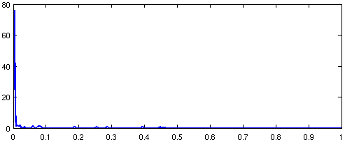
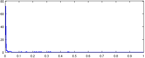
$J=30,K=3$	$J=120,K=3$
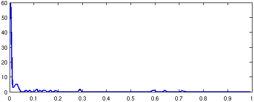
	intractable for Viterbi
$J=30,K=9$	$J=120,K=9$

Figure 1: Histograms of the number of videos with given ranges of relative error.

We limited the above experiment to sentences with no more than three content words because we wished to compare against the global optimum which can only be computed with the Viterbi algorithm. This process may become intractable with sentences with more than three content words, especially with large $J$. To demonstrate that the local-search approach can scale to process longer sentences we performed a second experiment. In this experiment, we processed six video clips with longer sentences. Fig. 2 illustrates the tracks produced for these video-sentence pairs, as derived from the indicator variables $p^{t,l}_{j}$. Note that for the example in the fourth row in Fig. 2, computing the global optimum with the Viterbi algorithm would take $15\times(120^{4}\times 3^{1})^{2}=5,804,752,896,000,000,000$ lattice comparisons. We estimate that this would take about 20 years on a current computer.

The person to the left of the traffic-cone carried the stool to the left of the trash-can slowly away from the traffic-cone.
56s, $T=12$, $I=2$, $J=30$, $K=3$, $L=5$, $W=10$
The person to the left of the trash-can carried the backpack to the left of the stool slowly towards the stool.
61s, $T=15$, $I=2$, $J=30$, $K=3$, $L=5$, $W=10$
The person to the left of the stool carried the trash-can slowly towards the traffic-cone.
129s, $T=15$, $I=2$, $J=30$, $K=9$, $L=4$, $W=8$
The person to the left of the trash-can carried the traffic-cone to the left of the backpack.
667s, $T=15$, $I=2$, $J=120$, $K=3$, $L=4$, $W=7$
The person to the left of the trash-can carried the traffic-cone.
520s, $T=15$, $I=2$, $J=120$, $K=3$, $L=3$, $W=5$
The person to the left of the trash-can picked up the traffic-cone to the right of the backpack quickly.
230s, $T=10$, $I=2$, $J=90$, $K=3$, $L=4$, $W=8$

Figure 2: Tracks produced by processing six video clips of varying lengths $T$ with the associated sentences of varying complexity $L$ and $W$, along with the running time in seconds to produce such with GT from the indicated number of detections $J$ per frame and word models of varying complexity $I$ and $K$. Best viewed on a color screen.

6 Related work

Lin et al. [20] present an approach for searching a database of video clips for those that match a sentential query. Implicit in this is a function that scores how well a video clip depicts a sentence or alternatively how well a sentence describes a video clip. That work differs from the current work in several ways. First, they run a tracker in isolation, independently for each object, before scoring a video-sentence pair. Here, we jointly perform tracking and scoring, and do so jointly for all tracks described by a sentence. This allows scoring to influence tracking and tracking one object to influence tracking other objects. Second, their scoring function composes only unary primitive predicates, each applied to a single track. Here, our scoring function composes multivariate primitive predicates, each applied to multiple tracks. This is what links the word meanings together and allows the entire sentential semantics to influence the joint tracking of all participants. Third, the essence of their recognition process (not training) is that they automatically find what they denote as $y_{uv}$. This maps tracks $v$ to (unary) arguments of primitive predicates $u$. Here, we solve a dual problem of automatically finding what we denote as $p^{l}_{j}$, a map from event participants $l$ to detections $j$. Fourth, they allow predicates to be assigned to a dummy track “no-obj” which allows them to ignore portions of the sentence. Here, we constrain the track collection to satisfy all primitive predicates contained in a sentence. Fifth, they adopt a “no coreference” constraint that requires that each nondummy track be assigned to a different primitive predicate. Here, we allow such. This allows us to process sentences like The person approached the backpack to the left of the chair that contain, in part, primitive predicates like $\textsc{approach}(\textbf{person},\textbf{backpack})\wedge\textsc{leftOf}(\textbf{backpack},\textbf{chair})$ where the track backpack is assigned to two different primitive predicates. Sixth, they do not model temporally-varying features in their primitive predicates. Here, we do so with HMMs.

The relaxed sentence tracker also shares some similarity in spirit with current research in image/video object co-detection/discovery [17, 18, 24, 30] based on object proposals [1, 14, 41]. The goal of this line of work is to find instances of a common object across a set of different images or video frames, given a pool of object candidates generated by measuring the ‘objectness’ of image windows in each image. This is done by associating a unary cost with each candidate to represent the confidence that that candidate is an object, and a binary cost between pairs of candidates to measure their similarity in appearance, resulting in a second-order MRF/CRF. Selecting the best candidate for each image constitutes a MAP estimate on this random field, and is usually relaxed to constrained nonlinear programming [18, 30], or computed by a combinatorial optimization technique such as tree-reweighted message passing [19, 24]. Except for its loopy graph structure, this formulation is analogous to detection-based tracking in Eq. 6. In contrast to the work presented here, prior work on object co-detection/discovery only exploits visual appearance—analogous to the term $f(b)$ in Eq. 6—and object-pair similarity—analogous to the term $g(b^{\prime},b)$ in Eq. 6—but not the degree to which an object track exhibits particular spatiotemporal behavior, as is done by the terms $h(k,b)$ and $a(k^{\prime},k)$ in the event tracker, Eq. 8, let alone the joint detection/discovery of multiple objects that exhibit the collective spatiotemporal behavior described by a sentence, as is done in the sentence tracker, Eq. 5.

7 Discussion

Siddharth et al. [26], Barbu et al. [4], and Yu and Siskind [39] present a variety of applications for the sentence tracker. Since the sentence tracker is simply a scoring function that scores a video-sentence pair, one can use it for the following applications:

focus of attention

Given a single video clip as input, that contains two different activities taking place with different subsets of participants, along with two different sentences that each describe these different activities, produce two different track collections that delineate the participants in the two different activities.

sentence generation

Given a video clip as input, produce a sentence as output that best describes the video clip by searching the space of all possible sentences to find the one with the highest score on the input video clip.

video retrieval

Given a sentential query as input, search a dataset of video clips to find that clip that best depicts the query by searching all clips to find the one with the highest score on the input query.

language acquisition

Given a training corpus of video clips paired with sentences that described these clips, search the parameter space of the models for the words in the lexicon that yields the highest aggregate score on the training corpus.

With the exception of the last use case, language acquisition, the other use cases all treat the sentence tracker as a black box. We have demonstrated a plug-compatible black box that takes the same input in the form of a video-sentence pair and produces the same output in the form of a score and a track collection. Since we have proven that the global optimum to the relaxed objective is the same as that for the original objective, and further empirically demonstrated that local search tends to find a local optimum that is qualitatively the same as the global one, one can employ this relaxed method to perform exactly the same first three uses cases as the original sentence tracker with identical, or nearly identical results. The chief advantage of the relaxed method is that it scales to longer sentences. More precisely, we demonstrate three distinct kinds of scaling:

1. Because the original sentence tracker had space complexity of $O(TJ^{L}K^{W})$ and time complexity $O(T(J^{L}K^{W})^{2})$ it was, in practice, limited to small $J$, typically at most 20. Here, we perform experiments that demonstrate scaling to $J=120$.

2. Similarly, the original sentence tracker was limited, in practice, to small $K$, typically at most 3. Here, we perform experiments that demonstrate scaling to $K=9$.

3. Similarly, the original sentence tracker was limited, in practice, to small $L$ and $W$, typically $L\leq 3$, i.e. at most three nouns in the sentence, and typically at most two words that have more than one state in their HMM. (Words that describe static properties, like nouns, adjectives, and spatial-relation prepositions, typically have a single-state HMM while words that describe dynamic properties, like verbs, adverbs, and motion prepositions, typically have multiple states.) Here, we perform experiments that demonstrate scaling to $L=5$ and $W=10$.

Since the method of Yu and Siskind [39] for the fourth use case, namely language acquisition, does not use the sentence tracker as a black box, extending our new method to this use case is beyond the scope of this current work.

8 Conclusion

The sentence tracker has previously been demonstrated to be a powerful framework for a variety of applications, both theoretical and potentially practical. It can serve as a model of grounded child language acquisition [39] as well as the basis for searching full-length Hollywood movies for clips that match rich sentential queries [4] in a way that is sensitive to subtle semantic distinctions in the queries. However, until now, it was impractical to apply in many situations that require scaling to complex sentences with many event participants. Our results remove that barrier.

References

- [1] B. Alexe, T. Deselaers, and V. Ferrari. Measuring the objectness of image windows. IEEE Transactions on Pattern Analysis and Machine Intelligence, 34(11):2189–2202, 2012.
- [2] S. Avidan. Support vector tracking. IEEE Transactions on Pattern Analysis and Machine Intelligence, 26(8):1064–1072, 2004.
- [3] A. Barbu, N. Siddharth, A. Michaux, and J. M. Siskind. Simultaneous object detection, tracking, and event recognition. Advances in Cognitive Systems, 2:203–220, 2012.
- [4] A. Barbu, N. Siddharth, and J. M. Siskind. Language-driven video retrieval. In CVPR Workshop on Vision Meets Cognition, 2014.
- [5] L. E. Baum. An inequality and associated maximization technique in statistical estimation of probabilistic functions of a Markov process. Inequalities, 3:1–8, 1972.
- [6] L. E. Baum and J. A. Eagon. An inequality with applications to statistical estimation for probabilistic functions of Markov processes and to a model for ecology. Bulletin of the American Mathematical Society, 73(3):360–363, 1967.
- [7] L. E. Baum and T. Petrie. Statistical inference for probabilistic functions of finite state Markov chains. The Annals of Mathematical Statistics, 37(6):1554–1563, 1966.
- [8] L. E. Baum, T. Petrie, G. Soules, and N. Weiss. A maximization technique occuring in the statistical analysis of probabilistic functions of Markov chains. The Annals of Mathematical Statistics, 41(1):164–171, 1970.
- [9] R. Bellman. Dynamic Programming. Princeton University Press, 1957.
- [10] M. Brand, N. Oliver, and A. Pentland. Coupled hidden Markov models for complex action recognition. In CVPR, pages 994–999, 1997.
- [11] A. E. Bryson, Jr. A steepest ascent method for solving optimum programming problems. Journal of Applied Mechanics, 29(2):247, 1962.
- [12] A. E. Bryson, Jr. and Y.-C. Ho. Applied optimal control. Blaisdell, Waltham, MA, 1969.
- [13] P. Chang, M. Han, and Y. Gong. Extract highlights from baseball game video with hidden Markov models. In ICIP, volume 1, pages 609–612, 2002.
- [14] M.-M. Cheng, Z. Zhang, W.-Y. Lin, and P. Torr. Bing: Binarized normed gradients for objectness estimation at 300fps. In CVPR, pages 3286–3293, June 2014.
- [15] A. Griewank. Who invented the reverse mode of differentiation? Documenta Mathematica, Extra Volume ISMP:389–400, 2012.
- [16] M. Han, A. Sethi, W. Hua, and Y. Gong. A detection-based multiple object tracking method. In ICIP, pages 3065–3068, 2004.
- [17] Z. Hayder, M. Salzmann, and X. He. Object co-detection via efficient inference in a fully-connected CRF. In ECCV, pages 330–345, 2014.
- [18] A. Joulin, K. Tang, and L. Fei-Fei. Efficient image and video co-localization with Frank-Wolfe algorithm. In ECCV, pages 253–268, 2014.
- [19] V. Kolmogorov. Convergent tree-reweighted message passing for energy minimization. IEEE Transactions on Pattern Analysis and Machine Intelligence, 28(10):1568–1583, 2006.
- [20] D. Lin, S. Fidler, C. Kong, and R. Urtasun. Visual semantic search: Retrieving videos via complex textural queries. In CVPR, pages 2657–2664, 2014.
- [21] G. M. Ostrovskii, Y. M. Volin, and W. W. Borisov. Über die Berechnung von Ableitungen. Wissenschaftliche Zeitschrift der Technischen Hochschule für Chemie, Leuna-Merseburg, 13(4):382–384, 1971.
- [22] J. Pearl. Reverend bayes on inference engines: a distributed hierarchical approach. In AAAI, pages 133–136, 1982.
- [23] J. Pearl. Probabilistic Reasoning in Intelligent Systems: Networks of Plausible Inference. Morgan Kaufmann Publishers Inc., San Francisco, CA, 1988.
- [24] A. Prest, C. Leistner, J. Civera, C. Schmid, and V. Ferrari. Learning object class detectors from weakly annotated video. In CVPR, pages 3282–3289, 2012.
- [25] P. Ravikumar and J. Lafferty. Quadratic programming relaxations for metric labeling and Markov random field MAP estimation. In ICML, pages 737–744, 2006.
- [26] N. Siddharth, A. Barbu., and J. M. Siskind. Seeing what you’re told: Sentence-guided activity recognition in video. In CVPR, 2014.
- [27] J. M. Siskind and Q. Morris. A maximum-likelihood approach to visual event classification. In ECCV, pages 347–360, 1996.
- [28] B. Speelpenning. Compiling Fast Partial Derivatives of Functions Given by Algorithms. PhD thesis, Department of Computer Science, University of Illinois at Urbana-Champaign, 1980.
- [29] T. Starner, J. Weaver, and A. Pentland. Real-time American sign language recognition using desk and wearable computer based video. IEEE Transactions on Pattern Analysis and Machine Intelligence, 20(12):1371–1375, 1998.
- [30] K. Tang, A. Joulin, L.-J. Li, and L. Fei-Fei. Co-localization in real-world images. In CVPR, pages 1464–1471, 2014.
- [31] A. J. Viterbi. Error bounds for convolutional codes and an asymtotically optimum decoding algorithm. IEEE Transactions on Information Theory, 13(2):260–267, 1967.
- [32] A. J. Viterbi. Convolutional codes and their performance in communication systems. IEEE Transactions on Communication Technology, 19(5):751–772, 1971.
- [33] Z. Wang, E. E. Kuruoglu, X. Yang, Y. Xu, and S. Yu. Event recognition with time varying hidden Markov model. In ICASSP, pages 1761–1764, 2009.
- [34] P. J. Werbos. Beyond Regression: New Tools for Prediction and Analysis in the Behavioral Sciences. PhD thesis, Harvard University, 1974.
- [35] J. K. Wolf, A. M. Viterbi, and G. S. Dixon. Finding the best set of K paths through a trellis with application to multitarget tracking. IEEE Transactions on Aerospace and Electronic Systems, 25(2):287–296, 1989.
- [36] B. Wu and R. Nevatia. Detection and tracking of multiple, partially occluded humans by Bayesian combination of edgelet based part detectors. International Journal of Computer Vision, 75(2):247–266, 2007.
- [37] J. Yamoto, J. Ohya, and K. Ishii. Recognizing human action in time-sequential images using hidden Markov model. In CVPR, pages 379–385, 1992.
- [38] J. S. Yedidia, W. T. Freeman, and Y. Weiss. Generalized belief propagation. In Proceedings of the Neural Information Processing Systems Conference, pages 689–695, 2000.
- [39] H. Yu and J. M. Siskind. Grounded language learning from video described with sentences. In ACL, pages 53–63, 2013.
- [40] S. Zhong and J. Ghosh. A new formulation of coupled hidden Markov models. Technical report, Department of Electrical and Computer Engineering, The University of Texas at Austin, 2001.
- [41] C. L. Zitnick and P. Dollár. Edge boxes: Locating object proposals from edges. In ECCV, pages 391–405, 2014.