Collaborative Randomized Beamforming for Phased Array Radio Interferometers

Abstract

The Square Kilometre Array (SKA) will form the largest radio telescope ever built and such a huge instrument in the desert poses enormous engineering and logistic challenges. Algorithmic and architectural breakthroughs are needed.

Data is collected and processed in groups of antennas before transport for central processing. This processing includes beamforming, primarily so as to reduce the amount of data sent. The principal existing technique points to a region of interest independently of the sky model and how the other stations beamform.

We propose a new collaborative beamforming algorithm in order to maximize information captured at the stations (thus reducing the amount of data transported). The method increases the diversity in measurements through randomized beamforming. We demonstrate through numerical simulation the effectiveness of the method. In particular, we show that randomized beamforming can achieve the same image quality while producing $40\%$ less data when compared to the prevailing method matched beamforming.

1 Introduction

The Square Kilometre Array (SKA) will form, upon completion, the largest and the most sensitive radio telescope ever built, consisting of millions of antennas over a total collection area of one square kilometer [Dewdney et al. (2009)]. The resultant data will be immense – on the order of one terabyte of data every second – equivalent to almost one tenth the total global internet traffic. The state of the art in engineering and algorithms for data collection, instrument calibration, storage, and imaging struggles to keep pace.

In addition to hardware optimization, tailored improved algorithms with lower data production are a promising solution. Thus, the work presently described was motivated by the need to reduce data as far up the processing chain as possible.

SKA will comprise different antenna types, dishes and phased arrays. The phased array is designed to attain a large field of view. Antennas are grouped into antenna stations where RF signals are received. These signals are then processed by beamforming, and sent to a central data processor for image creation through correlation and further beamforming [Wright (2002)].

For station beamforming, methods from array signal processing can be used to optimize different criteria. The strategy currently used in one SKA pathfinder, the Low Frequency Array (LOFAR) [Van Haarlem et al. (2013)], is matched beamforming [van der Veen and Wijnholds (2013)]. Antenna RF signals are summed after phase aligning the signal coming from an a priori chosen look direction. This can be seen as a matched spatial filter [Wijnholds (2010)], where the filter is matched towards the chosen direction. Another method used is minimum variance directionless response (MVDR) beamformer, equivalent to maximizing the ratio of signal power from a chosen direction to interference plus noise [van der Veen and Wijnholds (2013), Capon (1969)].

It is neither feasible nor desirable to send raw antenna time-series for correlation. Beamforming, mapping down signals from a higher to a lower dimensional space, is essentially lossy data compression distributed throughout the stations. Looked at it from that viewpoint, the following question naturally arises: how could one maximize the information content so as to reduce the data transmitted from stations to the central processor?

Thus, our goal is to reduce the amount of data and the complexity of the subsequent stages. Less data coming out of the stations means less traffic sent to the central data processor. Hence, an early reduction in the data yields savings in data transportation cost and the amount of processing in the later stages.

The organization of the paper is as follows. Section 2 describes beamforming at stations, including a description of the signal model. We then propose in Section 3 a collaborative beamforming technique for reducing data rates, and a sparse signal recovery formulation leveraging the proposed beamforming. Section 4 provides a numerical evaluation before conclusion in Section 5.

2 Beamforming at stations

2.1 Signal Model

Let $L$ denote the number of antennas and $Q$ the number of sources. Assume that celestial sources are in the far field, signals emitted by them are narrow band circularly-symmetric complex Gaussian processes, and that signals emanating from different directions in the sky are uncorrelated [Taylor et al. (1999)]. The signal received by the $L$ antennas, $\mathbf{x}(t):\mathbb{R}\rightarrow\mathbb{C}^{L}$, can be stated as

$$\mathbf{x}(t)=\sum_{q=1}^{Q}\mathbf{a}_{q}s_{q}(t)+\mathbf{n}(t),$$

where $s_{q}(t)\sim\mathcal{NC}(0,\sigma^{2}_{q})$ is the signal emitted by source $q$, $\mathbf{n}(t)\sim\mathcal{NC}(0,\sigma^{2}\mathbf{I})$ is the additive noise at the antennas, and $\mathbf{a}_{q}\in\mathbb{C}^{L}$ is the antenna steering vector towards source $q$ given by [van der Veen and Wijnholds (2013)]

$$\mathbf{a}_{q}=\begin{pmatrix}e^{-j\frac{2\pi}{\lambda}\mathbf{r}_{q}^{\top}\mathbf{p}_{1}}&e^{-j\frac{2\pi}{\lambda}\mathbf{r}_{q}^{\top}\mathbf{p}_{2}}&\cdots&e^{-j\frac{2\pi}{\lambda}\mathbf{r}_{q}^{\top}\mathbf{p}_{L}}\end{pmatrix}^{\top},$$ (1)

where $\lambda$ is the observation wavelength, $\mathbf{r}_{q}$ is the unit vector pointing at source $q$, and $\mathbf{p}_{1}$, $\cdots$ $\mathbf{p}_{L}$ are the positions of the antennas. This summation can be written as a matrix vector product

$$\mathbf{x}(t)=\mathbf{A}\mathbf{s}(t)+\mathbf{n}(t),$$

where $\mathbf{A}\in\mathbb{C}^{L\times Q}$ has its column $q$ equal to $\mathbf{a}_{q}$, and $\mathbf{s}(t):\mathbb{R}\rightarrow\mathbb{C}^{Q}$ has its $q$th element equal to $s_{q}(t)$.

In a wide number of scientific cases, the parameters of interest are the source intensities (signal variance) and positions. Because signals arriving at antennas are modeled as circularly symmetric complex Gaussian processes, the autocorrelation matrix is a sufficient statistic. Assuming the noise and the signals to be uncorrelated, we have the correlation matrix

$$\mathbf{R}=\mathbb{E}\left[\mathbf{x}(t)\mathbf{x}(t)^{\mathrm{H}}\right]=\mathbf{A}\mathbf{\Sigma_{s}}\mathbf{A}^{\mathrm{H}}+\mathbf{\Sigma_{n}},$$ (2)

where $\mathbf{\Sigma_{s}}=\mathop{\mathrm{diag}}(\sigma^{2}_{1},\sigma^{2},\ldots,\sigma^{2}_{Q})$ and $\mathbf{\Sigma_{n}}=\sigma^{2}_{n}\mathbf{I},$ are diagonal covariance matrices for the signal and noise respectively.

2.2 Beamforming

Here we lay the groundwork for explaining the beamforming methods described in Section 3. In particular, we will describe the hierarchical design of phased array radio interferometers, and then discuss the general issue of combining signals at station level and the current prevailing method.

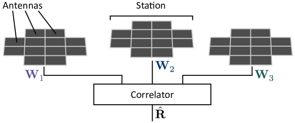
Figure 1: Hierarchical design of phased array radio telescopes. Groups of antennas are combined as stations.

In hierarchically designed phased array radio interferometers [Van Haarlem et al. (2013), Ellingson et al. (2009), Lonsdale et al. (2009)], multiple antennas are grouped according to geography into antenna stations, cf. Fig. 1. The positions and the orientations of the antennas are fixed. In order to scan different portions of the sky, individual antennas have a large field of view [Wijnholds (2010)], cf. Fig. 2. Sending all data received from all antennas for central data processing is costly. Hence, the data is typically reduced at stations by beamforming.

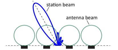
Figure 2: Antenna beams capture signals from a large region (green circles). Matched beamforming reduces the field of view and amplifies the signal coming from a particular direction.

The current prevailing method is matched beamforming, which points towards the center of a chosen region. Formally, say we choose a region centered around direction $\mathbf{r}_{0}$. Then, the signals are combined using a beamforming vector equal to the antenna steering vector towards $\mathbf{r}_{0}$. If all of the stations have the same layout – which is the case in modern radio interferometers, e.g., LOFAR [Van Haarlem et al. (2013)] – then all beamforming vectors are the same, leading to the same beam shape at each station.

One approach taken to introduce variations in beam shapes is to rotate the stations with respect to each other [Van Haarlem et al. (2013)]. These rotations may help to reduce grating lobes, whose positions are also rotated, and hence the signals outside the region of interest are averaged out.

Station beamforming can be viewed as linear operation on a $J$ dimensional signal, where $J$ is the number of antennas at the station. It is thus representable, for $M$ beams at the $k$th station, by matrix $\mathbf{W}_{k}\in\mathbb{C}^{J\times M}$. The beamformer output is then

$$\mathbf{y}_{k}(t)=\mathbf{W}_{k}^{\mathrm{H}}\left(\mathbf{A}_{k}\mathbf{s}(t)+\mathbf{n}(t)\right),$$

where $(\cdot)^{\mathrm{H}}$ denotes conjugate transpose. The correlation of two beamformed outputs is

$$\mathbb{E}\left[\mathbf{y}\mathbf{y}^{\mathrm{H}}\right]=\mathbf{W}^{\mathrm{H}}\mathbf{A}\mathbf{\Sigma}_{s}\mathbf{A}^{\mathrm{H}}\mathbf{W}+\mathbf{W}^{\mathrm{H}}\mathbf{\Sigma}_{n}\mathbf{W},$$ (3)

where $\mathbf{W}\in\mathbb{C}^{JL\times ML}$ is the block diagonal matrix containing the beamforming matrices of $L$ stations, and $\mathbf{A}\in\mathbb{C}^{JL\times Q}$ the response matrix of all antennas towards the $Q$ sources.

Let us study the output from a station $k$. Dropping the dependence on time for brevity, the signals at the antennas can be written as $\mathbf{x}_{k}=\mathbf{A}_{k}\mathbf{s}+\mathbf{n}_{k}$. Then $\mathbf{y}_{k}=\mathbf{w}_{k}^{\mathrm{H}}\left(\mathbf{A}_{k}\mathbf{s}+\mathbf{n}_{k}\right)$ for beamforming vector $\mathbf{w}_{k}$. The variance of the resulting signal is equal to

$$\mathbb{E}\left[\mathbf{y}_{k}\mathbf{y}_{k}^{\mathrm{H}}\right] =\sum_{q=1}^{Q}|\mathbf{w}_{k}^{\mathrm{H}}\mathbf{a}_{k,q}|^{2}\sigma^{2}_{q}+\sigma^{2}_{n}\|\mathbf{w}_{k}\|^{2},$$

where $\mathbf{a}_{k,q}$ stands for column $q$ of $A_{k}$. Hence, the variance of the signal from the $q$th source in the beamformer output of the $k$th station, $\sigma_{k,q}^{2}$, satisfies

$$\sigma_{k,q}^{2} =\big{|}\mathbf{w}_{k}^{\mathrm{H}}\mathbf{a}_{k,q}\big{|}^{2}\sigma^{2}_{q}\overset{(a)}{\leq}\big{\|}\mathbf{w}_{k}\big{\|}^{2}\big{\|}\mathbf{a}_{k,q}\big{\|}^{2}\sigma^{2}_{q},$$ (4)

where $(a)$ follows from Cauchy-Schwartz inequality. If we use the beamforming vector $\mathbf{w}_{k}=\mathbf{a}_{k,q}/\sqrt{J}$, a multiple of the antenna steering vector, then $(a)$ becomes an equality. This is the mathematical description of matched beamfoming. In that case, $\sigma^{2}_{k,q}=J\sigma^{2}_{q}$. Because this beamforming vector is of unit norm, the noise variance at beamformer output is equal to the variance $\sigma^{2}_{n}$ at a single antenna. Hence, the signal coming from the $q$th source is amplified with a factor of $J$ with respect to the noise.

Intuitively, narrowband signal coming from a particular direction reaches the antennas with phase delays. Matched beamforming aligns the phases of signals from a chosen direction and sums. Hence, the magnitude of the signal is maximized, whereas because noise is uncorrelated at antennas, it is not coherently combined.

3 Collaborative beamforming

We have seen that beamforming is essentially fixed/static at all stations. This is a waste. When all beam shapes are the same, we cannot use the magnitude information in sky image reconstruction, but are limited to the phase information resulting from geometric delays between stations. When stations use different beamforms, the correlation between two station outputs becomes

$$\mathbb{E}\left[\mathbf{y}_{k}\mathbf{y}_{m}^{\mathrm{H}}\right] =\sum_{q=1}^{Q}\mathbf{w}_{k}^{\mathrm{H}}\mathbf{a}_{k,q}\mathbf{a}_{m,q}^{\mathrm{H}}\mathbf{w}_{m}\sigma^{2}_{q}.$$ (5)

As $\mathbf{w}_{k}^{\mathrm{H}}\mathbf{a}_{k,q}\mathbf{a}_{m,q}^{\mathrm{H}}\mathbf{w}_{m}\in\mathbb{C}$, the correlation equals the sum of signal powers weighted by a constant that depends on station indices $k$ and $m$. Because of scaling variations, information is contained not only in the phases but also the signal magnitudes. This increase in information can then be exploited in non-linear signal recovery methods for the improvement of the quality of the resulting image.

Another benefit of using different beamforms is a reduction in the effects of potential systematic errors, such as grating lobes that result from fixed beam shapes.

3.1 Randomized beamforming

We can reduce the amount of data required for the same image quality (or conversely increase image quality for the same data rate). This is vital to make an SKA in the middle of the desert feasible. To get different beam shapes to act collaboratively for this purpose, beamforming vectors at antenna stations can be chosen from a random distribution. This method is inspired by compressed sensing, where random measurements were shown to preserve the information contained in sparse signals [Donoho (2006)].

The multiple beams at station $k$ can be described by a beamforming matrix $\mathbf{W}_{k}$ (cf. Section 3), which can be chosen with particular goals in mind:

1. generate each matrix element from an independent and identically distributed circularly-symmetric complex Gaussian random distribution with unit variance, and then normalize the columns to be of unit norm;

2. after generating the matrix as in R1, convolve each column with a fixed beam shaping filter and truncate the excess length (this attenuates signals coming from outside a chosen region of interest); or

3. generate the matrix by matched beamforming towards randomly chosen directions within the chosen region of interest.

Fig. 6 to Fig. 6 illustrate typical beams from these strategies. R1 has the largest beam variation. Vector normalization ensures the noise variance at beamformer output is equal to the antenna noise variance. However, depending on beam shape, we may attenuate the signal coming from a source as evident by (4). Hence, there is a trade off between beamform variations and signal power. When only interested in a small part of the sky in the presence of high measurement noise, using strategy R2 or R3 would be more promising.

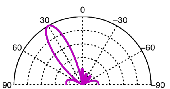
Figure 3: Matched beamforming

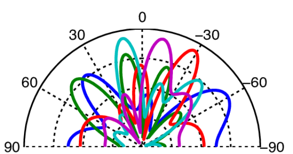
Figure 4: Randomization R1

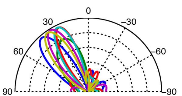
Figure 5: Randomization R2

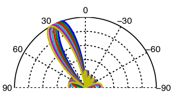
Figure 6: Randomization R3

3.2 Sparse signal recovery

Randomized beamforming is best tailored to a model-based sparse reconstruction algorithm. One such method is to maximize the likelihood of the observed data with respect to the parameters of the model [van der Veen and Wijnholds (2013)]. Radio astronomy parameters are, for point source models, the number of sources, positions and intensities of the sources, and the noise variance, which we represent by the set $\theta=\{Q,\mathbf{r}_{1},\cdots,\mathbf{r}_{Q},\sigma^{2}_{1},\cdots,\sigma^{2}_{Q},\sigma^{2}_{n}\}$. When the samples $\{\mathbf{X}[n]\}_{n=1,\cdots,N}$ are independent the maximum likelihood estimator is  [van der Veen and Wijnholds (2013)]

$$\operatorname*{\arg\!\min}_{\theta}\,\,\log\det(\mathbf{R}(\theta))+\operatorname{Trace}\bigl{(}\mathbf{R}^{-1}(\theta)\hat{\mathbf{R}}\bigr{)}.$$ (6)

where $\mathbf{R}(\theta)=\mathbf{A}(\theta)\mathbf{\Sigma(\theta)}\mathbf{A}^{\mathrm{H}}(\theta)+\sigma^{2}_{n}(\theta)\mathbf{I}$. In the model, the position parameters show up in a non-linear way, and the source intensities linearly. Given the source positions, the noise variance and assuming $\mathbf{A}$ admits a left inverse, the solution for the source intensities is equal to the diagonal elements of $(\mathbf{A}^{\mathrm{H}}\mathbf{A})^{-1}\mathbf{A}^{\mathrm{H}}\hat{\mathbf{R}}\mathbf{A}(\mathbf{A}^{\mathrm{H}}\mathbf{A})^{-1}-\sigma^{2}_{n}\mathbf{I}$ [Jaffer (1988)].

However, in the absence of a priori knowledge, problem (6) is hard to solve. In such cases, because a point source model imposes sparsity on the sky, sparse signal recovery methods, such as algorithms from compressed sensing literature can be used. To this end, we assume that the sources are on a two dimensional grid, denoted by $\{\mathbf{r}_{i}\}_{i=1,\cdots,N_{g}}$ where $N_{g}$ is the number of grid points. Define the matrix $\mathbf{A}_{g}\in\mathbb{C}^{L\times N_{g}}$ that has $k$th column equal to the antenna steering vector towards the $k$th grid point. Then, the signal intensity vector $\bm{\rho}_{s}\in\mathbb{R}^{N_{g}}$ can be estimated by least absolute shrinkage and selection operator [Tibshirani (1996)] (LASSO) by

$$\operatorname*{\arg\!\min}_{\bm{\rho}_{s},\rho_{n}}\|\hat{\mathbf{R}}-\mathbf{A}_{g}\mathrm{diag}\left(\bm{\rho}_{s}\right)\mathbf{A}_{g}^{\mathrm{H}}-\rho_{n}\mathbf{I}\|_{F}+\lambda\|\bm{\rho}_{s}\|_{1},$$ (7)

where $\|\cdot\|_{F}$ denotes the Frobenius norm, $\rho_{n}$ the noise variance, $\mathbf{I}$ the identity matrix, and $\lambda$ is a non-negative regularization constant.

From (3), if station $k$ uses beamforming matrix $\mathbf{W}_{k}\in\mathbb{C}^{J\times M}$, the correlation matrix becomes

$$\mathbf{R}=\mathbf{W}^{\mathrm{H}}\mathbf{A}\mathbf{\Sigma}_{s}\mathbf{A}^{\mathrm{H}}\mathbf{W}+\sigma^{2}_{n}\mathbf{W}^{\mathrm{H}}\mathbf{W},$$

where $\mathbf{W}\in\mathbb{C}^{LJ\times LM}$ is the block diagonal matrix containing the beamforming vectors. The signal recovery problem (7) is then

$$\operatorname*{\arg\!\min}_{\hat{\bm{\rho}}_{s},\hat{\rho}_{n}}\|\hat{\mathbf{R}}-\mathbf{W}^{\mathrm{H}}(\mathbf{A}_{g}\mathop{\mathrm{diag}}\left(\hat{\bm{\rho}}_{s}\right)\mathbf{A}_{g}^{\mathrm{H}}-\hat{\rho}_{n}\mathbf{I})\mathbf{W}\|_{F}+\lambda\|\hat{\bm{\rho}}_{s}\|_{1}.$$ (8)

This is the optimization used in the performance analysis.

4 Performance analysis

This section presents numerical simulation, showing the effectiveness of different station beamforms through randomization and image recovery using sparse signal recovery optimization (8).

For comparison of the simulation parameters to an actual radio telescope, we give the LOFAR High Band Antenna parameters. Made up of $48$ stations, the minimum and maximum baselines between each is $68$m and $1158$km respectively. Each station design is regular with $48$ receiving elements spaced $5$m apart, operating at $110$ MHz – $250$ MHz, which corresponds to wavelengths between $1.2$m to $2.7$m. This spaces the high band antennas and stations more than half a wavelength apart, creating grating lobes (cf. Section 2).

For simulation we fixed the number of stations $L$ to $4$, the number of antennas per station $J$ to $12$, and varied number of beams per station $M$. There were thus $LM(LM-1)/2=4M(4M-1)/2$ cross-correlations and $LM=4M$ autocorrelations.

The spacing between antennas within a station was $5$m, and the observation frequency $200$ MHz, resulting in an antenna spacing of approximately $3.3$ wavelengths. At each simulation run the stations were positioned within a disk of radius of $60$ wavelengths at random by approximating Poisson disk sampling using Mitchell’s best candidate algorithm [Mitchell (1991)]. This setting produced grating lobes, which does not adversely affect randomized beamforming. For best-case matched beamforming we attenuated them by rotating the stations with respect to each other (as done in LOFAR).

Source intensities were chosen from a Rayleigh distribution with second moment equal to $2$. The sources were contained in a circular region of the $l-m$ plane with radius $0.6$, a fairly large field of view. The locations were chosen on a grid of $600$ grid points by the best candidate algorithm to have them spread over the field of view. For matched beamforming when $M=1$, we directed the antennas to the center of the region of interest. When $M>1$, the antennas were matched to directions chosen by best candidate sampling to cover large area when combined.

We evaluated the performance of sky image reconstruction through mean squared error defined as

$$\mathrm{MSE}=\frac{1}{N_{\mathrm{I}}}\sum_{i=1}^{N_{\mathrm{I}}}\left(\bm{\rho}_{i}-\hat{\bm{\rho}}_{i}\right)^{2},$$

where $\bm{\rho}$ was the true sky image in the vectorized form, $\hat{\bm{\rho}}$ its estimate, and $N_{\mathrm{I}}=50$ the number of simulation runs.

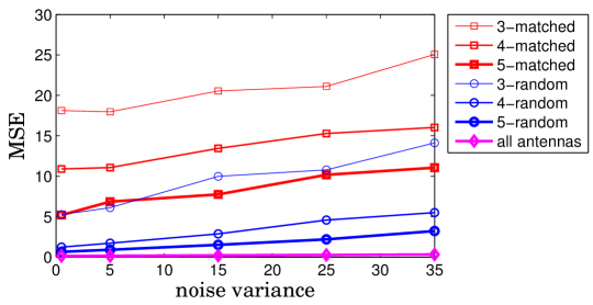
Figure 7: Reconstruction MSE for randomized and matched beamforming for different number of beams.

Fig. 7 shows the MSE obtained by randomized and conjugate matched beamforming, as well as a reference result obtained by correlation directly of every antenna signal pair. The number of beams per station ranged from $3$ to $5$. The number of sources was fixed to $20$. Both methods had similar behavior as the measurement noise varied. Using three beams per station with randomized beamforming had similar accuracy to using $5$ with matched beamforming.

Fig. 8 is the dual of Fig. 7. Noise variance was fixed while the number of beams per station changed. Except for the case of a single beam per station, the MSE performance of randomized beamforming was superior to matched beamforming. The diverse beam shapes generated by randomized beamforming results in different scaling of sky directions for different station pairs, and thus, helped resolve sources by also making use of the signal magnitudes. The diversity of the randomized beam shapes also explains the relative performance loss when using one beam. When correlating beamformed outputs from two stations, if low magnitude response directions from one beam overlap with high magnitude response directions from the other, the effective signal power is attenuated as can be seen in (5). Nevertheless, randomized beamforming improved rapidly and outperformed matched beamforming once there were at least two antennas per station.

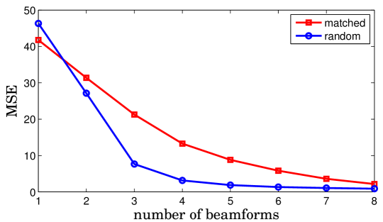
Figure 8: MSE for randomized and matched beamforming as a function of the number of beams per station. Noise variance $\sigma^{2}_{n}=25$.

Minimum number of beams necessary to meet MSE criteria for matched/randomized beamforming. Noise variance $\sigma^{2}_{n}=25$. Number of beams MSE Matched Random Rate ratio 10 $5$ $3$ 60 % 6 $6$ $4$ 67 % 3 $7$ $4$ 57 % 2 $8$ $5$ 63 %

Table 4 shows data compression rates from Fig. 8, specifically the required number of beams to go below an MSE level when using randomized and matched beamforming. As can be seen, the rate reduction for meeting the same MSE can be up to $43\%$.

5 Conclusions

We observed that beamforming in radio interferometry has yet to be fully exploited, its goals to date somewhat narrow in scope. It seemed attractive to maximize information in beamforming, getting beams to work in unison. Towards this end, we introduced a randomized beamforming strategy that increases measurement diversity. We showed that it can achieve substantial data reduction while preserving imaging quality. Sparse image reconstruction, a popular topic in radio astronomy, could additionally benefit from this “jumbling up” to a lower dimensional space.

We believe the SKA could benefit from a flexible, configurable beamforming architecture. There is always a resolution and computational trade-off to be made, and this would ideally be dictated by the science case. To which end, some of the future work we envisage includes developing further robustness in the presence of large measurement noise. Adaptation to other array signal processing problems, such as medical imaging or seismology, could also be a fruitful avenue of investigation.

References

- [1]
- Capon (1969) J Capon. 1969. High-resolution frequency-wavenumber spectrum analysis. Proc. IEEE 57, 8 (1969), 1408–1418.
- Dewdney et al. (2009) P E Dewdney, P J Hall, R T Schilizzi, and T J L W Lazio. 2009. The Square Kilometre Array. Proc. IEEE 97, 8 (Aug. 2009), 1482–1496.
- Donoho (2006) D L Donoho. 2006. Compressed sensing. IEEE Trans. Inf. Theory (April 2006), 1289–1306.
- Ellingson et al. (2009) S W Ellingson, T E Clarke, A Cohen, and others. 2009. The Long Wavelength Array. Proc. IEEE 97, 8 (2009), 1421–1430.
- Jaffer (1988) A G Jaffer. 1988. Maximum likelihood direction finding of stochastic sources: a separable solution. In IEEE Int. Conf. Acoust., Speech, and Signal Proc. New York, NY, 2893–2896.
- Lonsdale et al. (2009) C J Lonsdale, R J Cappallo, M F Morales, and others. 2009. The Murchison Widefield Array: Design Overview. Proc. IEEE 97, 8 (Aug. 2009), 1497–1506.
- Mitchell (1991) D P Mitchell. 1991. Spectrally optimal sampling for distribution ray tracing. SIGGRAPH Comput. Graph. 25, 4 (July 1991), 157–164.
- Taylor et al. (1999) G B Taylor, C L Carilli, R A Perley, and National Radio Astronomy Observatory (U.S.). 1999. Synthesis imaging in radio astronomy II. ASP Conf. Series.
- Tibshirani (1996) R Tibshirani. 1996. Regression shrinkage and selection via the lasso. J. Roy. Statist. Soc. Ser. B 58 (1996), 267–288.
- van der Veen and Wijnholds (2013) A J van der Veen and S J Wijnholds. 2013. Signal Processing Tools for Radio Astronomy. Springer New York, New York, NY, 421–463.
- Van Haarlem et al. (2013) M P Van Haarlem, M W Wise, A W Gunst, and others. 2013. LOFAR: The LOw-Frequency ARray. Astron. Astrophys. 556 (Aug. 2013), A2.
- Wijnholds (2010) S J Wijnholds. 2010. Fish-eye Observing with Phased Array Radio Telescopes. Ph.D. Dissertation. Delft University of Technology, Delft.
- Wright (2002) M C H Wright. 2002. A model for the SKA. Technical Report 16.